December 13

Our last class: students had tears. It was sad, sort of. Maybe.

I restated the Schwarz Lemma, declaring again that the proof was easy but also not easy (this doesn't really help, but it does reflect my feelings about the proof). I remarked that the Schwarz Lemma allowed us to solve a rather general extreme value problem:
If U and V are open subsets of the complex plane, and if a (respectively, b) are fixed points in U (respectively, V), we could wonder how much a holomorphic mapping from U to V taking a to b distorts Euclidean geometry. That is, if f:U-->V is holomorphic, with f(a)=b, then f "respects" conformal geometry. But what about the usual distance? If z is in U, what is the sup of |f(z)-b|? Or, if we are interested in infinitesimal distance, how large can |f´(a)| be? And what sort of functions, if any, actually achieve these sups?

The general scheme is to try to find biholomorhic mappings from D(0,1) to U and to V, taking 0 to a (respectively, b). Then composition changes the U, V and a, b problem to the hypotheses of the Schwarz Lemma. The composition then gives bounds on both |b-f(z)| and |f´(a)|. The functions which achieve these bounds are those which come from rotations. Problems 6 and 7 of the recent homework assignment illustrate this method.

I remarked that the family of mappings, defined for each a in D(0,1), sending z-->(z-a)/(1-conjugate(a)z, has already been introduced in this course. These are linear fractional transformations which send D(0,1) into itself and send a to 0. Thus the group of holomorphic automorphisms of D(0,1) is transitive. We can write all automorphisms if I understand the stabilizer of a point. I choose to "understand" those automorphisms f of D(0,1) which fix 0. By the Schwarz Lemma, these maps have |f'(0)|<=1. But the inverse of f is also an automorphism, and therefore 1=<|f'(0)|. So this means |f'(0)|=1, and therefore f(z)=e^i thetaz, a rotation, again using the Schwarz Lemma. So we now know that all holomorphic automorphisms of the unit disc are e^i theta[(z-a)/(1-conjugate(a)z]. Using this we can answer questions such as: what is the orbit of z₀, a non-zero element of D(0,1) (a circle centered at 0). I also mentioned an interesting geometric duality: D(0,1) is biholomorphic to H, the open upper halfplane of C. In D(0,1) the stabilizer of 0 is a subgroup of the biholomorphic automorphisms which is easy to describe: it is just the rotations, as we have seen. The transitive part of these mappings is not too easy to understand. In H, the transitive aspect of the automorphisms is nice. I can multiply by positive real numbers, and I can translate by reals. A combination of both of these can move i to any point of H. This double picture appears in many other situations.

Set	The group of holomorphic automorphisms
D(0,1), the unit disc	Linear fractional transformations of the form ei theta[(z-a)/(1-conjugate(a)z].
C, the whole complex plane	Affine maps: z-->az+b where a and b are complex, and a is non-zero
CP1, the whole Riemann sphere	All linear fractional transformations

How do we prove the result for C? Well, if f is a holomorphic automorphism of C, then f(1/z) has an isolated singularity at 0 (this is the same as looking at the isolated singularity of infinity of f(z), of course). Is the singularity removable? If it is, then a neighborhood of infinity is mapped by f itself to a neighborhood of some w. But that w is already in the range of f, so there is q with f(q)=w, and f maps a neighborhood of q to a neighborhood of w. Pursuit of this alternative shows that f cannot be 1-to-1, which is unacceptable. If f(1/z) has an essential singularity, then Casorati-Weierstrass shows also that f itself cannot be 1-to-1. Thus f(z) must have a pole at infinity. This pole should have order 1 or again we get a contradition.

The result for CP¹ uses the result for C. The CP¹ automorphism group certainly includes the linear fractional transformations. This group is (at least) transitive, so we can ask what the stabilizer subgroup of infinity is: that's az+b. And moving a point to infinity gives us all of LF(C)
Knowing the automorphism groups is really nice because of the following major result, which includes the Riemann Mapping Theorem:

The classical uniformization theorem
Any connected simply connected Riemann surface is biholomorphic with D(0,1) or C or CP¹.

This result is difficult to prove. The Riemann Mapping Theorem asserts that a simply connected open proper subset of C is biholomorphic with D(0,1). The uniformization theorem implies that the universal covering surface of any (connected) Riemann surface is one of D(0,1) or C or CP¹ and therefore we can study "all" Riemann surfaces by looking at subgroups of the Fundamental Group. For more information about this please take the course Professor Ferry will offer next semester.

I then discussed and proved a version of the Schwarz Reflection Principle. I showed how this could be used to analyze the automorphisms of an annulus, and how it could be used to see when two annuli were biholomorphic. I will write more about this when I don't need to rush off and give a final exam. Finally, Ms. Zhang applied the Schwarz Reflection Principle to verify a famous result of Hans Lewy, that there is a very simple linear partial differential equation in three variables with no solution. For further information about this, please link to the last lecture here.

December 8

It was a rapid day in Math 503, as the instructor tried desperately to teach everything he should long ago have discussed.

First, I wanted to simplify the argument principle so that I could use it more easily. I will make the following assumptions, which I will call S ("S" for "simplifying assumptions")

1. U is an open subset of C and f is holomorphic in U.
2. C is a closed curve in U, and C is homotopic to a constant in U.
3. If z₀ is not on C, and z₀ is in U, then either n(C,z₀)=1 (I'll call these z₀'s "inside C") or n(C,z₀)=0.
4. No zeros of f lie on C.

If I knew (officially) ...
If we accepted the Jordan curve theorem, then the following facts could be used:
If C is a simple closed curve in the plane (such a curve is a homeomorphic image of the circle, S¹) then C\C (the complement of C in the plane) has two components. One component is the unbounded component. If z₀ is in that component, then n(C,z₀)=0. Now let w be one of either +1 or -1. This statement is then true for one of the values: for all z₀'s in the other component, n(C,z₀)=w (the same w for all z0's in this other component). w=+1 if C goes around its inside the "correct" way, and w=-1 if it is reversed.
Certainly this would simplify S. In fact, for most applications, the curve is usually a circle or the boundary of a rectangular region, and the topological part of S is easy to check.

Theorem Assume S. Then _C[f´(z)/f(z)] dz=the number of zeros of f which lie inside C (where the zeros are counted with multiplicity).
This result uses S to eliminate the winding numbers in the statement of the argument principle, of course. I should mention here, in correct order, another consequence of the proof of the argument principle.

Suppose g(z) is also holomorphic in U. What do I know about the possible singularities of g(z)[f´(z)/f(z)]? Remember that [f´(z)/f(z)] has a singularity only at z₀ which is a zero of f(z), and there it looks locally like k/(z-z₀)+holomorphic. This is a simple pole with residue k. Now multiplying by g(z) doesn't create more singularities. It merely adjusts those of [f´(z)/f(z)]. If g(z) has a 0 at z₀ then g(z)[f´(z)/f(z)] is holomorphic at z₀. Otherwise, g(z)[f´(z)/f(z)] still has a simple pole at z₀ with residue kg(z₀. Therefore the Residue Theorem applies:
Theorem Assume S and that g(z) is holomorphic in U. Then _C[f´(z)/f(z)] dz=SUM_{z is a zero of f inside C, counted with multiplicity}g(z).
Notice that if z₀ is a 0 of f inside C and g(z₀)=0, then both sides of this formula happen to contribute 0 to the integral (left) and to the sum (right).
I have most often seen this used when g(z)=z^k with k a positive integer, and C some "large" curve enclosing all of the zeros of f. The result is then the sum of the k^th powers of the roots of f, which can be useful and interesting. For example, when one is considering symmetric functions of the roots, these sums are important.

Rouché's Theorem Assume S. Suppose additionally that g(z) is holomorphic in U, and that for z on C, |g(z)|<|f(z)|. Then the number of zeros of f inside C is the same as the number of zeros of f+g inside C.
Proof: Suppose t is a real number in the interval [0,1]. Then f(z)+tg(z) has the following property:
If z is on C, |f(z)+tg(z)|>=|f(z)|-|tg(z)|=|f(z)|-t|g(z)|>=|f(z)|-|g(z)|>0. Therefore f(z)+tg(z) is never 0 for z on C (both f(z) and f(z)+g(z) can't have roots on C), and the function
(t,z)-->f(z)+tg(z) is jointly continuous on [0,1]xU and holomorphic in the second variable, and never 0 when the second variable is on C. Thus the integral _C[{f(z)+tg(z)}´/{f(z)+tg(z)}] dz is a continuous function of t. But for each t, by the argument principle, this is an integer. A continuous integer-value function on [0,1] (connected!) is constant. Comparing t=0 (which counts the roots of f) and t=1 (which counts the roots of f+g), we get the result.

Comment The instructor tried to describe an extended metaphor: this resembled walking a dog around a lamppost with the length of the leash between the dog and person less than the distance of the person to the lamppost. Students were wildly enthusiastic about this metaphor. (There may be a sign error in that sentence.) The metaphor is discussed here and here and here. The pictures are wonderful. You can print out postscript of the whole "lecture" by going here and printing out the "first lecture".

Berkeley example #1
Consider the polynomial z⁵+z³+5z²+2. The question is: how many roots does this polynomial have in the annulus defined by 1<|z|<2? I remarked that we would apply Rouché's Theorem to |z|=1 and to |z|=2. The difficulty might be in deciding which part of the polynomial is f(z), "BIG", and which is g(z), "LITTLE".
C is |z|=1 Here let f(z)=5z². Then |f(z)|=5 on C, and |g(z)|=|z⁵+z³+2|<=|z|⁵+|z|³+2=4 on C. Since 4<5, and f(z) has 2 zeros inside C (at 0, multiplicity 2), we know that f(z)+g(z), our polynomial, has 2 zeros inside C.
C is |z|=2 Here let f(z)=z⁵. Then |f(z)|=32 on C, and |g(z)|=|z³+5z²+2|<=|z|³+5|z|²+2=8+20+2=30 on C. Since 30<32, and f(z) has 5 zeros inside C (at 0, multiplicity 5), we know that f(z)+g(z), our polynomial, has 5 zeros inside C.
Therefore the polynomial has 3=5-2 zeros on the annulus.

Comments First, as we already noted, the Rouché hypothesis |g(z)|<|f(z)| does prevent any zeros from sitting "on" C. That's nice. A more interesting observation is that this verification of the crucial hypothesis "|g(z)|<|f(z)| for all z on C" was actually implied by a much stronger statement:
that the sup of |g(z)| on C was less than the inf of |f(z)| on C. This stronger statement is usually easier to prove than the pointwise statement in many simple examples. But those who are wise enough to do analysis may well have situations where the pointwise estimate may be true without the uniform inequality being correct.

Berkeley example #2
Consider 3z¹⁰⁰+e^z. How many zeros does this function have inside the unit circle? Here on C, |z|=1. Thus |3z¹⁰⁰|=3 on C, and |e^z|=e^Re z<=e on C. Since e<3, the hypotheses of Rouch&ecute;'s Theorem are satisfied (with BIG=3z¹⁰⁰ and LITTLE=e^z). Since 3z¹⁰⁰ has a zero at 0 with multiplicity 100, I bet that 3z¹⁰⁰+e^z has 100 zeros inside the unit disc.
The Berkeley problem went on to ask: are these zeros simple? For those who care to count, this is asking for the cardinality of the set of solutions to 3z¹⁰⁰+e^z=0 inside the unit disc. A zero is not simple if it is a zero of both the function and the derivative of the function. So we should consider the system of equations:
3z¹⁰⁰+e^z=0
300z⁹⁹+e^z=0
The solutions to these (subtract and factor!) are z=0 and z=100. 100 is outside the unit disc. And notice that z=0 is not a solution of the system (of either equation, and it should be a solution of both!). Thus 3z¹⁰⁰+e^z=0 has 100 simple solutions (each has multiplicity 1) inside the unit disc!

I tried to explore how roots of a polynomial would change when the polynomial is perturbed. If p(z) is a polynomial of degree n (n>0) then we know (Fundamental Theorem of Algebra) that p(z) has n roots, counted with multiplicity. Now look at the picture. The smallest dots represent roots of multiplicity 1, the next size up, multiplicity 2, and the largest dot, multiplicity 3. (I guess, computing rapidly, that n=11 to generate this picture.) Now suppose that q(z) is another polynomial of degree at most n, and q(z) is very small in some sense. The only sense I won't allow is to have q(z) uniformly small in modulus in all of C (because then [Liouville] q(z) would be constant).
Where are the roots of p(z)+q(z)? In fact, what seems to happen is that when q(z) is very small, the roots don't wander too far away from the roots of p(z). Things can be complicated. The roots of multiplicity 2 could possibly "split" (one does, in this diagram) or the root of multiplicity 3 could split completely. How can we prove that this sort of thing happens?
Well, suppose we surround the roots of p(z) by "small" circles. Since all the roots of p(z) are inside the circles, |p(z)| is non-zero on these circles, and (finite number of circles, compactness!) inf|p(z)| when z is on any of these circles is some positive number, m. Now let q(z) be small. I mean explicitly let's adjust the coefficients of q(z) so that |q(z)| has sup on the set of circles less than m. Then the critical hypothesis of Rouché's Theorem is satisfied, and indeed, the roots of p(z)+q(z) are contained still inside each circle, exactly as drawn.

Certainly one can make this more precise. But I won't because I am in such a hurry. But I will remark on this: if we consider the mapping from Cⁿ⁺¹ to polynomials of degree<=n (an (n+1)-tuple is mapped to the coefficients), then for a dense open subset of Cⁿ⁺¹, the polynomial has n simple roots (consider the resultant of p and its derivative). On this dense open set, it can be proved that the roots are complex analytic functions of the coefficients. An appropriate version of the Inverse Function Theorem proves this result and it is not difficult but isn't part of this rapidly vanishing course.

I the stated
Hurwitz's Theorem Suppose U is a connected open subset of C, and {f_n} is a sequence of holomorphic functions converging to the function f uniformly on compact subsets of U. If each of the f_n's is 1-to-1, then ...
STOP STOP STOP!!!
Look at some examples. If U is the unit disc, consider f_n(z)=(1/n)z. Then these f_n's do converge u.c.c. to the function f(z)=0 (for all z). Hmmmm ... But if f_n(z)=z+(1/n) in the unit disc, these f_n's converge u.c.c. to z. These two behaviors are the only possible alternatives. O.k., let's go back to the formality of the math course:

Hurwitz's Theorem Suppose U is a connected open subset of C, and {f_n} is a sequence of holomorphic functions converging to the function f uniformly on compact subsets of U. If each of the f_n's is 1-to-1, then either f is 1-to-1 or f is constant.
Comment In other words, either the darn limit function is quite nice, or the limit function collapses entirely. In practice, it is usually not that hard to decide which alternative occurs.
Proof Well, suppose f is not constant. I'll try to show that f is 1-to-1. If f(z₁)=f(z₂)=w (where the z_j's azre distinct), then I will look at U\f^-1(w). Since f is not constant and U is connected, we know that (discreteness!) U\f^-1(w) is a connected open set. It is pathwise connected. Use this fact to connect z₁ and z₂ by a curve which (other than its endpoints!) does not pass through f^-1(w). Inside this curve, f(z)-w has two roots. But then f_n(z)-w has two roots for n very large (since the curve is a compact set, etc.). But this conclusion contradicts the hypothesis that f_n is 1-to-1. So ... we are done.

For example, Hurwitz's Theorem plays an important role in many proofs of the Riemann Mapping Theorem, where the candidate for the "Riemann mapping" is a limit of some sequence of functions, and then (because, say, the limit candidate has derivative not 0 at a point) the limit must be 1-to-1. But we have no time for this. (A famous mathematic quote [or pseudoquote, because it is exaggerated] is "I have not time; I have not time" ... here is a good reference.)

What follows is a remarkable result which I should have presented when I discussed the Maximum Modulus Principle.
Schwarz Lemma Suppose f is holomorphic and maps D(0,1) to D(0,1). Also suppose f(0)=0. Then
|f´(0)|<=1, and for all z in D(0,1), |f(z)|<=|z|.
If also either |f´(0)|=1 or there is a non-zero z₀ in D(0,1) so that |f(z₀)|=|z₀|, then f is a rotation: there is theta so that f(z)=e^i thetaz for all z in D(0,1).
Proof The proof has several notable tricks which I am sure I could not invent. First, "consider" g(z)=f(z)/z. This is fine away from 0. But, actually, since f(0) is assumed to be 0, g has a removable singularity at 0. Hey! Wow!! What should g(0) be? The limit of f(z)/z as z-->0 (remembering that g(0)=0!) is actually f´(0). So I will remove g's singularity at 0 by defining g(0) to be f´(0). O.k., and now we "work":
First notice that since g is holomorphic, by Max Mod, the sup of g on the set where |z|<=s occurs where |z|=s. So if |z|<=r and r<s, then |g(z)|<=|g(somewhere that |z|=s)|={|f(that z)/that z|}=1/s for s>=r and s<1. 1/s for r<s<1 has least upper bound 1. Therefore |g(z)|<=1 for all z in D(0,1). This establishes that claim that
|f´(0)|<=1, and for all z in D(0,1), |f(z)|<=|z|.
If either of these inequalities is an equality, then by Max Mod, the g function must be a constant (surely a constant with modulus equal to 1). Since g is a constant with modulus 1, f must be z multiplied by a constant of modulus 1, and this is a rotation.

That's the story. but I should remark that this proof, very short, very simple, seems (to me!) to be also very subtle. I have read the proof and read the proof and ... I was a coauthor on a paper which proved a version of Schwarz's lemma for Hilbert space, and used the lemma to verify some neat things, and I still am not entirely confident I understand the proof. Oh well. Next time I hope to give some very simple consequences.

I claimed that this proof was correct, or at least more correct than the one I offered in class. Mr. Matchett read it and found two misprints. Oh well.

December 6

Mr. Peters kindly discussed a wonderful sum of Gauss which can be evaluated using residues. Mr. Trainor kindly discussed a method using the Residue Theorem which can evaluate exactly (in terms of "familiar" constants) such sums as the reciprocals of the even integer powers. Here, are fourteen proofs of the Pi²/6 fact written by Robin Chapman.

I first advertised Rouché's Theorem, which I asserted allows us to hope that roots don't wander too far when their parent polynomials change a bit. This would be proved from the Argument Principle.

Suppose f is meromorphic in an open subset U of C. I showed that for z₀ in U, f'(z)/f(z) is k/(z-z₀)+h´'(z)/h(z) where h(z) is a non-zero holomorphic function near z₀. Using this I was able to state a version of the argument principle, having to do with the line integral of f´(z)/f(z) in U over a closed curve which did not pass through any poles or zeros of f and which was nullhomotopic in U. This integral can also be interpreted as the net change of the arg(f(z)) as z travels around the closed curve: the net number of times the curve's image wraps around the origin. This is, I asserted, the beginning of degree theory.

I will apply this to prove Rouché's Theorem next time, at which time I also hope to announce the real time of the final exam. Sigh.

Final exam
We discussed the Final Exam some more. This exam will be approximately as long and difficult as the midterm. The method of the exam will be the same. The exam will be given, I hope, on Friday, December 17, at 1:10, in SEC 220.

December 1

I did the last two integrals. I found the residue of something with a double pole. And I completely correctly computed the last integral, a result of Euler's. I used an interesting contour. I tried to do the problem as I imagine a good engineering student might do it (a really good student would use Maple or Mathematica!). As I mentioned in class, the full rigorous details of this integral are shown on three pages of Conway's text.

I just tried, very briefly, to do the last integral as I imagined Euler might have done, the way a physics person might (ignoring all that stuff about limits, integrals, differentiation, etc.). So I set F(c)=₀^infinity[x^-c/(1+x)]dx=Pi/sin(Pi c) and then I computed F(1/2) (this was easy to do explicitly using elementary calculus). Then I tried to compute F´(c). My desire was to get an ordinary differential equation for F. I was unable to do this. Maybe someone can help me. Maybe I should instead have looked for ome other kind of equation for F(c).

I derived yet another version of the Cauchy Integral Formula (the final version for this course, assuming that C is a closed curve in an open set U, f is holomorphic in U, and z is in U but not on C. Then _Cf(w)/(w-z) dw=n(C,z)f(z). This is a direct consequence of the Residue Theorem, recognizing that the function f(w)/(w-z) (a function of w) is holomorphic in U\{z}, and has a simple pole at z with residue equal to f(z).

Then I tried to verify the beginning of the Lagrange inversion theorem, sometimes called the Lagrange reversion theorem. I first asked what we could say about f:U-->C if f were 1-to-1. After Mr. Matchett told me that I seemed to be from Mars, I realized that I had forgotten to indicate that f was holomorphic. Now we could say something. But first I gave a real example ("real" refers here to the real numbers):
If f(x)=x³ then f is certainly smooth (real analytic!) and 1-to-1. The inverse map is not smooth at 0, of course.
Can this occur in the "holomorphic category"? Well, no: if f is locally 1-to-1, then f' is not 0, so (setting g equal to the inverse of f) g'(w)=1/f'(z) where f(z)=w. And g is holomorphic.

Then after much confusion and correction by students, I tried to compute the integral of sf´(s)/(f(s)-w) over a small circle centered at z. The Residue Theorem applies. The integrand is 0 only when f(s)=w. By hypothesis, this only occurs when s is z. The applicable winding number is 0. The pole at z is simple since f´ is never 0. Thus the residue is a residue at a simple pole. Here we need the limit of (s-z)[sf´(s)/(f(s)-w)] as s-->z. But we can recognize (s-z)/(f(s)-w) as the difference quotient upside-down. So the limit is 1/f´(z), and the limit of (s-z)[sf´(s)/(f(s)-w)] as s-->z is just z, which is g(w).

Therefore for sufficiently small r, _|w-z|=r [sf´(s)/(f(s)-w)] dw=g(w) if f(z)=w.

The significance of this result whose consequences applied to power series are frequently used in combinatorics, is that the operations on the integral side (the left-hand side above) are all involving f, while the right is just g.

I hope on Monday to cover Rouché's Theorem after Mr.Peters and Mr. Trainor, magnificent heros, speak.

Monday, November 29

Volunteers wanted!

Since I am tired, I would like two (2) volunteers to each prepare 15 minutes worth of Wednesday's lecture. One volunteer would discuss Gaussian sums. This is specifically Theorem 1 on p.82 of the text, N2. The discussion of this example occupies pp.82-84. One volunteer would discuss a neat method of finding sums of certain series. This is exercises 217 and 218 (first equation) and maybe 219.1 and 219.2 of N2. Any volunteers should send me e-mail. Thank you.

I restated the Residue Theorem and discussed again some idea of the proof. The residue of a function f(z) at an isolated singularity located at p is the constant a so that f(z)-a/(z-p) has a primitive in D(p,epsilon)\{p}. So the residue measures the obstacle to having a primitive.

The remainder of the (so-called) lecture was devoted to computational examples.

1. Use the Residue Theorem to verify that _|z|=2{1/([sin(z)]²cos(z))}dz=0.
   Here we needed to learn where, say, sin(z)=0. I "expanded" sin(x+iy) using the addition formula (true for real numbers, therefore by the indentity theorem for complex numbers). Then I found some residues.
2. Use the Residue Theorem to verify that _|z|=1{[sin(z)]/[z⁴(z²+2)]}dz=-(2/3)Pi  i
   In these computations I kept emphasizing that all we needed was the (-1) coefficient of the Laurent series, and that all formal manipulation was fine and could be justified. The Laurent series coefficient needed was unique.
3. Use the Residue Theorem to compute ₀^2Pi dt/[1-2pcos(t)+p²]
   Here the "secret" is to change the interval of integration [0,2Pi] into the unit circle, |z|=1, then put z=e^it, so dz/(iz)=dt, and cos(t) becomes [z+z^-1]/2. Then if p<1, the answer is 2Pi/sqrt(1-p²) (one residue at a simple pole) while if p>1, you need a residue at a different simple pole, and the answer is 2Pi/sqrt(p²-1).
4. Use the Residue Theorem to compute _-infinity^infinity dx/(1+x²
   This can be computed by elementary methods: it is Pi. Otherwise, we consider the contour I_R+S_R where I_R=[-R,R] and S_R is the upper semicircle, center 0 and radius R. For R>1, the Residue Theorem allows us to compute the integral over the closed curve of the function f(z)=1/(1+z²). On I_R, as R-->infinity, the integral goes to PV_-infinity^infinity1/(1+x²)dx but since the integrand is even (or since the integrand is L¹) the PV (principal value) is the same as the integral itself. The integral on S_R is easily estimated by the ML inequality. It is PiR/(R²-1) and, as R-->infinity, this-->0.
5. Make it fancier: _-infinity^infinity (cos(sx)/(1+x²)dx where s>0
   I tried to explain why the use of f(z)=(cos(sz)/(1+z²)) would not likely be successful (the M of the S_R would get too big, since cosine in the upper halfplane is sinh(y) more or less. So a trick is needed. We consider f(z)=e^isz/(1+z². Then when z=x+0iy, f(z)=e^isx/(1+x²)=(cos(sx)+i sin(sx))/(1+x²), and integrating over I_R makes the sine term go away. We can use the Residue Theorem, and estimation of |e^isz| for y>0 and s>0 shows that this is <=1.
   I asked what to do when s<0, and got some answers. In fact, for s real, the integral _-infinity^infinity (cos(sx)/(1+x²)dx is Pi e^-|s|. The absolute value is caused by 1/(1+x²) being L¹ but not having |x|/(1+x²) in L¹.
6. Next time: ₀^infinitydx/(x²+a²)²=Pi/(4a³)
   This won't be too hard.
7. And, next time, ₀^infinity[x^-c/(1+x)]dx=Pi/sin(Pi c).
   This is a bit more intricate and needs an interesting contour.

Monday, November 22

I went over Cauchy's Theorem again (no, I won't let it go, since it is a principal result of the subject). Again, I asserted the consequence that in a simply connected open subset of C, holomorphic functions which are never 0 have holomorphic logarithms. From this follows the existence of holomorphic n_th roots for such functions.

In a connected open set, if a holomorphic function has a log, then it will have exactly a countable number of logs, and these will differ by 2Pi integer. I made a similar remark about the number of different n^th roots (if at least one such function existed).

Increasing Mr. Trainor's disappointments
In addition to the possible failure of log mapping complex multiplication to complex addition (mentioned last time) I defined A^B to be e^Blog(A). It then turns out that (A^B)^C is hardly ever equal to A^BC. I think you may run into trouble if you try A=B=C=i, for example.
log i is i(Pi/2), so iⁱ is e^(i(Pi/2)i)=e^-Pi/2. Now (e^-Pi/2)ⁱ is e^i(-Pi/2)=-i. But iⁱ²=i^-1=-i. Darn! It seems they are the same! Please find an example where they are different.

A child's version of the Residue Theorem
We start with a function f holomorphic in D(0,1)\{0}. And a closed curve C in D(0,1)\{0}. What can we say about _Cf(z) dz?
Since f is holomorphic in A(0,0,1), I can write a Laurent series for f: f(z)=SUM_n=-infinity^infinitya_nzⁿ. Now let g(z)=SUM_n=-infinity^infinitya_nzⁿ-a_-1/z. Then g(z) has a primitive in D(0,1)\{0}: G(z)=SUM_n=-infinity^infinity(a_n/(n+1))zⁿ⁺¹ (n NOT equal to -1!). This is because we proved we can integrate term-by-term in the series (except for n=-1). So _Cf(z) dz=_Ca_-1/z dz. The number a_-1 is called the residue of f at 0. What about _C1/z dz. This is called the winding number of C about 0, n(C,0).

What values can _C1/z dz have?
If we go back to our definition of the integral (selecting discs, primitives, etc., then we see that _C1/z dz will be SUM_j=1ⁿlog_j(C(t_j))-log_j(C(t_j-1)). Now log_j is a branch of logarithm in D(z_j,r_j). The real parts of the logs are all the same. The imaginary parts differ by at most some multiple of 2Pi i. Since the real parts all cancel cyclically (remember, this is a closed curve, so C(a)=C(t₀)=C(t_n)=C(b), the differences are all 2Pi i multiples of an integer. Therefore the values of _C1/z dz are just in 2Pi iZ.
Please note that I gave a rather different impression of this proof in class. In particular, I seemed almost to insist that I needed to give a formula for the branch of logarithm in D(z_j,r_j). This meant that I needed to give a formula for argument in that disc. I got into trouble trying to be precise. In fact, all I really needed was the knowledge that a branch of log existed, and a complete description of the possible values of log(z). I knew those things and could use them to complete the proof as shown above. I didn't need to compute further.

The winding number
Suppose now C:[a,b]-->C is a closed curve, and the complex number w is not in C([a,b]). Then the winding number of C with respect to w, n(C,w), is (1/[2Pi i]) _C(1/[z-w])dz.

Properties of the winding number

• The winding number is an integer.
  The proof of this is exactly like what we did for 1/z in the discussion above.
• Any integer can be a winding number.
  Suppose n is an integer. If C is the curve defined on [0,2Pi] given by the formula C(t)=e^ni t and w is 0, then C is a closed curve, and w is not in the image of C, and n(C,w) will be n.
• n(C,w) is constant in the components of the complement of C([a,b]).
  Well, n(C,w) is a Cauchy transform, and is therefore holomorphic in the complement of C([a,b]). Since it is integer-valued, and the integers have the discrete tolopology, n(C,w) is constant on components.
• For large w, n(C,w) is 0.
  Indeed, we know that n(C,w) is essentially a Cauchy transform, and so if C([a,b]) is contained in D(0,R) then n(C,w) is an integer for |w|>R and n(C,w)-->0 as w-->infinity. So n(C,w)=0 for such w.
  Note Certainly, it is possible for n(C,w) to be 0 without w being outside of the image of C (create an example!).
• If C₁ and C₂ are closed curves which are homotopic (as closed curves!) in C-{w}, then n(C₁,w)=n(C₂,w)
  This is a direct consequence of one of the versions of Cauchy's Theorem.

A grownup's version of the Residue Theorem
The hypotheses are a bit long. First, we need an open subset U of C, and a discrete subset, P, of U with no accumulation point in U. (Depending on your definition of "discrete in U", the last requirement may not be needed, but I'd like to specify it anyway.) Now we need f, a function holomorphic in U\P. And we need a closed curve C defined on [a,b] so that C([a,b]) is contained in U\P, and so that C is nullhomotopic in U (homotopic to a constant through closed curves in U).
The conclusion evaluates _Cf(z) dz. It equals 2Pi i multiplied by the SUM_{w in P} n(C,w)res(f,w).
Note The residue of f at w, res(f,w), is the coefficient of 1/(z-w) in the Laurent series of f in a tiny deleted disc at w: D(w,epsilon)-{w}.

So this theorem turns out to be a very powerful result, with many applications both in theory and in practical computation. But it isn't even clear that the sum described in the theorem is finite! But it is. Since C is nullhomotopic, there is a homotopy, H:{a,b]x[0,1]-->U which is a continuous map so that H(_,0)=C and H(_,1) is a point. Let K=H({a,b]x[0,1]). Since H is continuous, K is a compact subset of U. Now P has only finitely many points in K. If w is not in K, then n(C,w)=0 since n(H(_,1),w)=0 and we use the last remark about winding numbers above. So the sum is indeed finite. (I think this is tricky: we don't need the Jordan curve theorem or anything, just some cleverness!).

Proof Suppose w_j is the list of all w's which are both in P and in K, for j=1,...n (a finite set!). Let S_j(z) be the sum of the negative terms in the Laurent series of f at w_j. From the theory of Laurent series, we know that this series converges absolutely and uniformly on compact subsets of C\{w_j}, and so is holomorphic on C\{w_j}. The difference f-SUM_j=1ⁿS_j has removable singularities in K: consider them removed. Now by Cauchy's Theorem, _Cf(z)-SUM_j=1ⁿS_j(z) dz has integral 0. Therefore we only need to compute the integral of S_j(z) over C to complete our proof. But, just as in the child's version above, the "higher" terms (that is, (z-w)^-(integer>1)) integrate to 0 since they have primitives in C\{w_j}. The only term that remains gives us exactly 2Pi i n(C,w_j)ref(f,w_j). And we're done.

I'll spend the next week giving applications (computation of definite integrals) and proving powerful corollaries (Rouché's Theorem) of the Residue Theorem.

Wednesday, November 17

Today's vocabulary

recondite 1. (of a subject or knowledge) abstruse; out of the way; little known. 2. (of an author or style) dealing in abstruse knowledge or allusions; obscure. abstruse hard to understand; obscure; profound. prolix lengthy; tedious. trenchant (of a style or language etc.) incisive, terse, vigorous. incisive mentally sharp; acute. méchant (French) nasty (said of a person) (Certainly applies to the instructor!)

We deduced various forms of Cauchy's Theorem (I believe I wrote three of them). To do this, I remarked that if the image of a closed curve was inside an open disc, then the integral of a holomorphic function around that closed curve is 0 (a consequence of our method last time: we can take one open disc for the collection of discs, and one primitive, and as partition, just the endpoints of the interval. Then the the sum is 0.) (Proof suggested by Mr. Nguyen.)

Now I used something (uniform continuity, compactness, Lebesgue number, stuff) to see the following: if H:{a,b]x[0,1]-->U is continuous (for example, a homotopy!) then there are integers m and n and a collection of open discs, D(z_jk,r_jk) for 1=<j<=n and 1=<k<=m, in U so that (with t_j=a+j(b-a)/n and s_kk=k/m) H([t_j-1,t_j]x[s_k-1,s_k]) is contained in D(z_jk,r_jk). This is so darn complicated! Well, it means that we can break up the rectangle {a,b]x[0,1] into little blocks so that the image of each little block fits inside an open disc contained in U. But then the integral of f(z) dz (for f analytic in U) over the image of the boundary of that block must be 0 (using Mr. Nguyen's fact). And it is easy (?!) to see that the sum of over all the blocks shows that, for closed curves S and T with images in U, homotopic through closed curves, gives _Sf(z) dz=_Tf(z) dz. And this was one of the three forms of Cauchy's Theorem I wrote.

An open subset of U is simply connected if every closed curve is homotopic to a constant. Another version of Cauchy's Theorem is that the integral of any holomorphic function around a closed curve in a simply connected open set must be 0. (By the way, it saves worrying about things if we also assume in this discussion that the open sets are connected.).

Now I asked for examples of simply connected sets, and I was given the disc. My homotopy of a closed curve to a point (nullhomotopic) just involved a linear interpolation of the curve to a point, so apparently I only needed that the open set be convex, or even just star-shaped.

Now I asked for an example of an open connected set which was not simply connected. Here we used the annulus, A(0,0,2), as U. We claimed that the boundary of the unit circle was a simple closed curve (true) not homotopic to a point in U. Why? Well, the integral of 1/z around that curve is 2Pi i, not 0. Since 1/z is holomorphic in U, we know that the curve is not nullhomotopic. This is really cute. (I mentioned, which is true but definitely not obvious, that we only need to use 1/(z-a) to "test" for nullhomotopy.)

I defined the first homotopy group of a topological space, based at a point, as the quotient of the set of loops through the point modulo the equivalence relation, homotopy, and using as the group operation, addition is "follow one curve by another". There are then lots of details to check. The fundamental group is a topological invariant (two homeomorphic spaces have isomorphic fundamental group). This group can be isomorphic to the identity (true when U is simply connected). Or it can have a whole copy of Z in it (take U=A(0,0,2), using "going around the unit circle n times" and integration to show that none of these curves is homotopic to each other). In fact, the group can be complicated and not obvious. A "twice-punctured plane" (say C\{+/-1}, which is sort of topologically the lemniscate) has Fundamental Group equal to the free product on two generators, and this group is not commutative. This can't be checked by Cauchy's Theorem, since the integral evaluated on a "curve" which is made from commutators will always be 0. This needs a result called Van Kampen's Theorem. So: enough of that stuff (topology).

O If U is simply connected and f is holomorphic in U, then f has a primitive in U: a function F, holomorphic in U, so that F´=f.
This is true because we saw that such an F exists exactly when the integral of f around closed curves in U is 0, and this hypothesis is fulfilled due to Cauchy's Theorem.

1 If U is simply connected and if f is holomorphic in U and never vanishes, then f has a holomorphic log: there is g holomorphic in U with e^g=f.
By reasoning backwards (we did this before) we know how to walk forwards. So: consider k=f´/f, holomorphic in U since f never vanishes. Now this function has a primitive, K, and we can consider G=e^K. The function f/G (G can't be 0 since exp is never 0) has derivative 0 (just compute algorithmically). Since (I hope U is connected!) f/G is constant, and neither f nor G is zero, f/G is a non-zero constant. But then there is a constant q so that exp(q)=f/G and so f=e^K-q and we have our holomorphic log.

How many holomorphic logs are there? In fact, if g₁ and g₂ are holomorphic logs of f on U (a connected U) then e^g₁-g₂=1 and therefore the continuous function g₁-g₂ takes U to 2Pi(the integers). But the latter set is discrete, so therefore the function g₁-g₂ must be constant. Thus we see that if a function has a holomorphic log, then it has infinitely many holomorphic logs, and these functions differ by integer multiples of 2Pi i.

An "undergraduate" problem
Look at the domain pictured on the right, the domain G (heh, heh, heh). I claim that this open set is connected, does not include 0, and is also simply connected. A totally rigorous proof of all of these statements would need, of course, a really careful description of G, which I have not given. Well, but "of course" you can see G is connected (it is arcwise connected: a curve is drawn connecting 1 to 2 in G, and other curves can be drawn to connect any pair of points in G). And maybe (almost "of course") you can see that G is simply connected: put a closed curve in G, and you can almost see how to untwist it (always staying in G!) and get it to shrink to a point (in G). Now the function z is holomorphic and non-zero in G. So z has a holomorphic log, L(z). I know therefore that e^L(z)=z in G. But, wait, since we earlier (September 13) explicitly solved e^w=z. Thus we know that L(z) is a complex number whose real part is ln(|z|) (the "natural log" of z), and its imaginary part is arg(z), where arg(z) is one of the arguments of z. Now we are allowed by our previous discussion to specify L(z)'s value at one point (up to a multiple of 2Pi i. So I will declare that L(1) is 0. Now I ask what L(2) must be. Well, it is a complex number whose real part is ln(2). What is its imaginary part? First, an approximate answer: if you "walk along" the dashed red path from 1 to 2 and pay attention to arg, and start with arg(1)=0, then you will end up with arg(2)=2Pi. That's because arg increases, and we travel totally around 0: L(2)=ln(2)+2Pi i. More rigorously, we could assert that we have a C¹ function whose derivative obeys what the derivatives of arg should be, and integrate the darn thing as the path goes from 1 to 2. We'll end up with the same increase in arg. So although we can get a holomorphic log on G, it may not agree very much with the standard log on G intersect R. Mr. Trainor asked about the implications for the formula log(ab)"="log(a)+log(b). I put quotes around the equality because it is not likely to be true, and if you ever want to use it, you should worry about its validity. Yes, the complex numbers are wonderful, but their use could also be ... complicated.

As we saw before, if we have a holomorphic log, we then have holomorphic square roots and cube roots and ... we will continue to discuss this next time.

Monday, November 15

Go to the colloquium
when you know that the talk will be comprehensible. And interesting. Better, bring work with you and sit in the back. Try diligently to understand for 5 minutes, and then ... do what you would like to do.

What now?

1. Cauchy's Theorem An appropriate version of Cauchy's Theorem (usually stated with homotopy or homology) is customary. In fact, the versions we have already are probably enough for almost all applications. But ... the homology version may generalize better to higher dimensions, but the best way to approach the homology version is with an analytic result called Runge's Theorem, which we will not have time to prove. I will verify a homotopy version of Cauchy's Theorem, and the pictures are nice.
2. The Residue Theorem We follow Cauchy's Theorem with a suitable version of the Residue Theorem, which has many applications ranging from the routinely computational (now used in machine computation as in Maple) to theoretical uses in studying, say, the Fourier transform.
3. Schwarz I should prove a version of the Schwarz Lemma, which gives an amazing approach to extremal problems. If time permits, I will state and verify the Schwarz Reflection Principle and show how it gives a distinctly modern result in PDE's (analysis of Lewy's equation).

Preliminary definition (with lack of specificity)
I first tried to define homotopy. Two closed curves S and T in U, defined on [a,b], are homotopic if there is a map H:{a,b]x[0,1]-->U so that H(_,0)=S and H(_,1)=T.
Analysis Well, we'd better have H continuous or else we don't have too much information about the relationship between S and T (observation contributed by Mr. Nguyen). And, maybe we'd better have c_v=H(_,v) be a closed curve for every v in [0,1] or unlikely things can happen as I tried to draw in class (for example, without this condition, a closed curve around 0 in D(0,1)\{0} could be homotopic to a constant). (Contributed by Mr. Nandi.)

Now I want to proved Cauchy's Theorem, and this should say something like: if S and T are homotopic closed curves (with a continuous homotopy through closed curves) and f is holomorphic in U, then the integral of f around S is equal to the integral of f around T. Well, what we could do is try to study the function _cvf(z) dz as a function of v (v is in [0,1]) and see (somehow!) that this function is constant. Unfortunately, there is a serious technical difficulty. Although the curves S and T are supposed to be piecewise C¹ curves in our previous definitions, the homotopy H which gives the curves c_v and these curves need not be more than continuous.

Giuseppe Peano did not invent the piano, nor did he invent the integers although he formulated a nice set of axioms for them (but Kronecker stated, "God created the integers, all else is the work of man."). Peano showed that there were continuous surjections between intervals in R and regions in R². Here is more information. Please note that these maps are not 1-1. But it does seem difficult to imagine that we could integrate f(z) dz over a random continuous curve.

There are various ways to analyze the integral over H(_,v) now. We can use simplicial approximation and get piecewise linear curves, or we can approximate by convolving with a C^infinity function to get nice smooth curves. I will follow a more primitive method. (There is a joke in that sentence.)

We will compute such integrals if we realize that we can take advantage of the holomorphicity of f(z). In differential geometry language, we will use the fact that f(z) dz is closed and is therefore locally exact to define the integral.

Creation of the "data" used to "integrate"
Suppose S:[a,b]-->U is a continuous map. Then K=S([a,b]) is compact in U. We can in fact find a partition for [a,b]: a=t₀<t₁<...t_n-1<t_n=b so that S([t_j-1,t_j]) is always inside D(z_j,r_j) which is an open disc in U. This follows from compactness and uniform continuity, I think. In each D(z_j,r_j) we know that f has a primitive, F_j, so F_j´(z)=f(z) in D(z_j,r_j) (contributed by Mr. Matchett earlier in the course). Then, if P is the partition and D is the collection of open discs and F is the collection of primitives, we define
I(f,S,P,D,F) to be SUM_j=1ⁿF_j(S(t_j))-F_j(S(t_j-1)).
I changed notation from S used in class to I here because I can't write the Greek letters (such as sigma) in html.

Now there are a sequence of observations and lemmas.

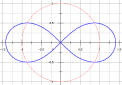Lemon	Lemming	Lemniscate

#1 Consistency with the previous definition
If S is a piecewise C¹ curve, then the value of I(f,S,P,D,F) is the same as _Sf(z) dz.
We can write the integral as a sum of integrals along the various peices of the curve, that is, S restricted to [t_j-1,t_j]. But in each of those we already saw that since the curve is inside an open disc, the line integral of f can be computed by taking the difference F(S(t_j))-F(S(t_j-1)) where F is any antiderivative of f. Therefore the old definition agrees with each piece of the "new" definition.

#2 The choice of primitives doesn't matter
We can change primitives. Thus if G_j and F_j are both primitives of f in D(z_j,r_j), then the functions differ by a constant. Thus F_j(S(t_j))-F_j(S(t_j-1)) and G_j(S(t_j))-G_j(S(t_j-1)) agree. Therefore the sum we have defined does not depend on selection of F.

#3 The choice of discs doesn't matter
We can change discs. That is, suppose we know that S([t_j-1,t_j]) is inside both D(z_j,r_j) and D(w_j,p_j) with corresponding primitives F_j and G_j. Then S([t_j-1,t_j]) is contained in the intersection of the discs. This intersection is an intersection of convex open sets and is hence convex and open. Therefore the intersection is connected and open, and the primitives F_j and G_j of f must again differ by constants. So F_j(S(t_j))-F_j(S(t_j-1))=G_j(S(t_j))-G_j(S(t_j-1)) again and the sum we have defined does not depend on selection of D.

It is also true that the sum doesn't depend on the partition, but here some strategy (perhaps borrowed from the definition of the Riemann integral) is needed. I'll first "refine" a partition by one additional point.

#4 Adding a point to a partition doesn't change the sum
If P is one partition: a=t₀<t₁<...t_n-1<t_n=b so that S([t_j-1,t_j]) is always inside D(z_j,r_j) which is an open disc in U, and F_j is the corresponding primitive, and if w is a point in [a,b] which is not equal to one of the t_j's, then look at the corresponding data. The only difference is F^*_j+1(S(t_j))-F^*_j+1(S(w))+F^*_j(S(w))-F^*_j(S(t_j-1)) in the partition with w, and F_j(S(t_j))-F_j(S(t_j-1)) without w. But we can add and subtract F_j(S(w)) to the latter sum, and notice that F_j and F^*_j are both antiderivatives, again, of the same function (f) in a connected open set (again, a disc or the intersection of two discs). And the same is true of the other "piece". So there is no difference if we make the partition "finer": add one more point.

#5 The choice of partitions doesn't matter
Two partitions P and Q give the same result for their corresponding sums. This is because the partition R which is the union of P and Q is a common refinement, and is obtained from each of P and Q by adding one point "at a time". So by the previous result, the sums must be the same.

Lemma Suppose S is a continuous curve from [a,b] to U, and f is holomorphic in U. Then I(f,S,P,D,F) does not depend on P or D or F when the choices are made subject to the restrictions described above. Also, if S is a piecewise C¹ curve, this sum is equal to the integral of f on S.
Therefore, we extend the definition previously used for piecewise C¹ curves by calling this sum _Sf(z) dz.

Next time I will formally state a homotopy version of Cauchy's Theorem, and prove it using this lemma.

Return of the exam; discussion
I returned the exam. I emphasized that I wished students to do as well as possible. For example, it is perfectly permissable to study with each other, and therefore there is little reason not to do as well as possible on problems which I have previously shown to you. I also asserted that I will not give more exam problems on topology. I have tried.

Wednesday, November 10

Midterm exam

Monday, November 8

I talked a bit more (but only a bit more!) about Riemann surfaces. I remarked that:

If S is a compact and connected Riemann surface, then every holomorphic function on S is a constant.
Why is this? If F:S-->C is holomorphic, then |F| is a continuous function on S, and hence |F| achieves is maximum, at some point p in S. But then in a coordinate chart around p, we have a holomorphic function which has a local maximum in modulus. In that chart, the function F must therefore (Max Modulus Theorem) be a constant. What now? We have a function, F, which is constant in some non-empty open subset of S. We can use connectedness and the identity theorem to conclude that F is constant on S.

Thus for compact connected Riemann surfaces, S, H(S) is just C. What about M(S)? This is (equivalently) either the functions on S which locally look like (z-p)^{some integer}(non-zero holomorphic function). M(S) is a field, and always contains the complex numbers, so it is a field extension of C. Such fields are called function fields. In the case of CP¹, we saw that all rational functions give elements of M(CP¹). If f is a meromorphic function on CP¹, then the pole set of f is finite (the pole set is discrete and CP¹ is compact). We can multiply by an appropriate product of (z-p_j)^-1's to cancel the poles. So we get a holomorphic function: that is, a constant. Thus every element of M(S) corresponds to a rational function. The field extension of C is a simple transcendental extension by z.

Now I looked at L, the set of Gaussian integers, in C. A Gaussian integer is n+mi where n and m are integers. L is a maximal discrete subgroup. L is certainly an additive subgroup and its elements are discrete. If we include another element of C, the subgroup is either isomorphic to L or it is not discrete in C. Sigh. I think that is what I meant by maximal here.

Anyway, give C/L the quotient topology. Then C/L is a compact topological space. It is homeomorphic to S¹xS¹, a torus. C/L is also a Riemann surface, with coordinate charts provided by just the identity.

Functions on C/L correspond to functions on C which are doubly-periodic: f(z)=f(z+i)=f(z+1) for all z in C. If such a function is entire, then since its values are all given on the unit square, the function is bounded and thus by Liouville must be constant. So again we have proved that H(T) consists of constant functions. What about M(T)?

Notice that the function z in M(CP¹) has a single pole of order 1. Is there such a function in M(T)? If f(z) has a pole at a, then imagine a being in the center of a "period parellelogram" for T: so a is inside the square formed by 0, 1, i, and 1+i. Now f(z)=b/(z-a)+a linear combination of non-negative integer powers of (z-a) (just the Laurent series). We can integrate f over the boundary of the unit square. But we've seen that this integral is 2Pi i b. But the integral over the sides of the square is also 0, since the two horizontal sides cancel because the function is i periodic and the two vertical sides cancel because the function is 1 periodic. Thus b=0. There is no meromorphic function on T with one simple pole.

Please note that there are complex two-dimensional manifolds which have no non-constant meromorphic functions. So it might be possible that there are no non-constant meromorphic functions on T. But there are many, and they are called, classically, elliptic functions.

Creating a silly elliptic function
We look at a function and "average it" by L. In this case, consider G(z)=SUM_{n+m i in L}1/(z-(n+m i))⁷. Let's see why this function converges "suitably". If A is fixed, then let's split the sum:
G(z)=SUM_{n+m i in L}1/(z-(n+m i))⁷= SUM_{In+m i in L}1/(z-(n+m i))⁷+ SUM_{IIn+m i in L}1/(z-(n+m i))⁷ where the first sum is over those n+mi which are inside D(0,2A) and the other sum, the "infinite tail", is over those which are outside. The infinite sum can be estimated:
|SUM_{IIn+m i in L}1/(z-(n+m i))⁷|<= SUM_{IIn+m i in L}1/|z-(n+m i)|⁷.
For z in D(0,A), this is overestimates (using the triangle inequality) by SUM_II(1/2)(n²+m²)^-7/2. But this last sum converges. So by the Weierstrass M-test, we know that G(z) in D(0,A) is SUM_I, a rational function having a pole of order 7 in each period parellelogram, plus a holomorphic function. Thus G(z) does converge to a non-trivial elliptic function, with a pole of order 7 on T.

We generalized this reasoning: 7 is not special. By using a two-dimensional integral test, we saw that for degree 3 and above, the analog of G(z) will then converge.

The most famous elliptic function
This is analog of G(z) when the exponent is 2. But then the sum we needed using our method doesn't converge absolutely! Weierstrass defined his P-function (the P should be a German fraktur letter) in the following way:
P(z)=1/z²+SUM'[1/(z-(n+im))²]-[1/(n+im)²].
Here the ' in the sum indicates that we add over all n+im in L except for the n=0 and m=0 term. Then this sum does converge suitably. Why is this? The difference [1/(z-(n+im))²]-[1/(n+im)²] does cancel out the worst part of the singularity at n+im. If you do the algebra, the difference (when |z| is controlled) is not O{(sqrt(n²+m²))^-4} which diverges, but is less.

It turns out that P'(z)=P³+(constant)P+(another constant). This result is proved using the Residue Theorem and fairly simple manipulations. Then more can be shown: an element f of M(T) can be written as R(P)+Q(P)P', where R and Q are rational functions in one variable. Thus the field M(T) is an algebraic extension of degree 3 of a purely transcendental extension of C. Wonderful!

My next and maybe concluding goals in the course are to verify suitably broad versions of Cauchy's Theorem and the Residue Theorem. I wished everyone good luck in their algebra exam.

Wednesday, November 3

I will continue to provide a gloss of the notes I wrote a decade ago. According to the online dictionary, gloss means

1. [Linguistics][Semantics]
   a. an explanatory word or phrase inserted between the lines or in
   the margin of a text.
   b. a comment, explanation, interpretation, or paraphrase.
2. a misrepresentation of another's words.

PDF of page 10 of my old notes
I wanted to show that elements of LF(C) map {lines/circles} transitively. Let me try to say this more precisely. If W is a subset of the complex numbers which happens to be a (Euclidean) line or circle, and if T is in LF(C), then I wanted to show T(W) is a (Euclidean) line or circle. In fact, even this is inaccurate, because I need to look at the closure of W as a subset of CP¹. In CP¹, a "straight line" has infinity in its closure, and if you look at the stereographic picture, lines are just circles on the 2-sphere which happen to go through infinity.

As I mentioned in class, a direct proof, computing everything in sight, is certainly possible. It might be easier to understand the proof if we examine the structure of LF(C). It is a group. And so, taking advantage of this group structure, we need only verify the statement to be proved for generators of this group, since it will then be true for all products of these generators.

PDF of page 11 of my old notes
On this page I complete the proof that the elements suggested as generators of LF(C) indeed were such, and I began to describe the elements of the set {lines/circles} in what I hoped was a useful way. Note for later comments, please, that the description given (see the bottom of page 11 and the top of page 12) depends upon 4 real parameters.

PDF of page 12 of my old notes
Now we compute how the generators found for LF(C) interact with the description of {lines/circles}. Translations and dilations are simple. It is worth pointing out, as I tried to, that inversion in a circle (a point goes to another point, and the result is on the same line with the center of the circle, with the product of the distances to the center being the square of the radius) preserves circles. (The fixed point set of such an inversion is exactly the circle itself.) The map z-->1/z is inversion in the unit circle foloowed by reflection across the real axis.

PDF of page 13 of my old notes
I went on a bit now, which I did not in the notes. I remarked that Euclid "proved" that three distinct points in the plane were contained in a unique element of {lines/circles}. An efficient proof, I think, would use linear algebra. However, I can't immediately see a simple reason that the determinant of

( a conjugate(a) a*conjugate(a) )
( b conjugate(b) b*conjugate(b) )
( c conjugate(c) c*conjugate(c) )

I think n then paused for examples. Let's see: I transforms the boundary of the unit disc, |z|=1, to |z-{3/2}|=1/2 and then changed that circle to something line |z-5|=2. I noted that although circles (and lines) get changed as proved, the center of a circle does not necessarily get moved to the center of the corresponding circle. If this were assumed, other computations would be simpler but also would also be wrong.

I tried to map the region between the imaginary axis and the circle |z+1|=1 (a circle with center at -1 and radius 1, tangent to the imaginary axis) to the interior of the unit circle. We found that 0 had to be mapped to infinity. And we further discussed the situation.

A parameter count
LF(C) is triply transitive on CP¹, and, in fact, each element of LF(C) is determined by its values on three distinct points (this can be used to define the cross ratio, an interesting invariant attached to LF(C)). But 3 complex parameters is the same as 6 real parameters. An element of {lines/circles} is determined by 4 real parameters as was previously observed. What happens to the extra numbers? Of course, this is the same as asking what subgroup of LF(C) preserves a particular element of {lines/circles}. Let's look at R and ask which T's in LF(C) preserve R. We can guess some T's such that T(R) is contained in R (and thus T(R) would have to be equal to R!). T(z)=z+1, or even T(z)=z+b, for b real. Thus if T(0) is not 0, we can pull T(0) back to 0 with a reverse translation (I am trying to build up enough elements to generate the subgroup!). If T(0)=0, then T(1) is something else, say, T(1)=a, with a not zero. Thus we now have the subgroup of T's given by the formula T(z)=az+B with a not 0 and a and b real. But, wait, we have ignored a prominent member of R's closure in CP¹: infinity. So far we know T(infinity)=infinity. But that need not be the case. Look at T(z)=1/z, which surely preserves R (in CP¹!). If we now think about it, we've got everything:
The collection of elements of LF(C) which preserve R is generated by az+b (a,b real, a not 0: the affine group) and z-->1/z.
The parameter count is now correct, since a and b are the two extra parameters we lacked. The z-->1/z is an extra transformation, and it exchanges the upper and lower half planes.

Because of z-->1/z as in the last example, if your interest is mapping regions to regions (this often happens in complex analysis and its applications) then you must check that the appropriate interiors are mapped correctly. Now again, try to map the region between the imaginary axis and the circle |z+1|=1 (a circle with center at -1 and radius 1, tangent to the imaginary axis) to the interior of the unit circle. If we take z-->1/z, then the imaginary axis becomes the imaginary axis, and the circle |z+1|=1 becomes Im z={1/2}. The domain which is our region of interest is mapped to the strip between these lines (so 0<Im z<{1/2}) but officially we do need to check, at least minimally!

I played some simple linguistic games discussing mappings of CP¹.

• Holomorphic
  The only holomorphic functions on CP¹ are constants. These are the holomorphic mappings from CP¹ to C. If we follow such a candidate map by z-->|z| then immediately we see that the map must be bounded, so, in one of the stereographic coordinate charts Liouville's Theorem applies, and the map is bounded. Alternatively, in one of the coordinate charts, the map has a local maximum in modulus and is therefore constant (Maximum Modulus) and by the Identity of Analytic Continuation, is constant over all of CP¹.
• Meromorphic
  The meromorphic functions on CP¹ are the holomorphic maps of CP¹ to CP¹ (how about that language!). There are some. For example, z is one of them, and z has one zero at 0 and one pole at infinity. The function (z⁵+3)/z⁷⁸ is another. It has a simple zero at each of the 5^th roots of -3 (simple because the derivative of z⁵+3 doesn't vanish at any of them) and it has a zero of order 78-5=73 at infinity. It has a pole of order 78 at 0. In fact, each meromorphic function is a rational function of z, and the number of poles and zeros always coincide. The field of meromorphic functions on CP¹ coincides with the field C with one transcendental element adjoined ("z").

Monday, November 1

As papers covering a table were moved recently in my home, a fortuitous discovery occurred: I found notes written for a previous (1994) instantiation of Math 503. I found only two objects related to Math 503: the notes for a lecture about projective space and the final exam. I tried to give a lecture today following the notes. Although I talked very fast, I could not come near finishing the lecture! I will try to scan the notes tomorrow and display them here, together with some commentary. It was fun to see what I thought was important a decade ago, and contrast this with my current prejudices (opinions?).

PDF of page 1 of my old notes
Discussed why one wants projective space. A reference is made to Bezout's Theorem, a classical result in algebraic geometry. Like many classical results in that area, Bezout's Theorem is more of an idea rather than just one theorem. Here are two sources for further information, one written by Professor Watkins, an economics faculty member at San José State, and one written by Aksel Sogstad of Oslo, Norway.

PDF of page 2 of my old notes
Here's the description of the projective space of a vector space. The idea is simple and useful.

• Math physics Here is a quote from web page:
  We will think of a quantum state as a (normalized) vector |v> in H. For math folks, we are in effect working in complex projective space, normalizing to 1 so that the probabilities make sense.
  And from another:
  "The physical significance of the projective Hilbert space is that in quantum theory, the wave functions psi and Lambda Psi represent the same physical state, for any Lambda not 0."
• Combinatorics There are a very rich set of references. Here is only one. When we consider a vector space over a finite field, there are lots of things to count.
• Topology, geometry There are too many references!

PDF of page 3 of my old notes
This presents a way to get the topologies on the projective spaces when the field is R or C. The spheres "cover" the projective spaces. In the case of R, the "fiber" of the mapping is two points, +/- 1, while for C, the "fiber" (inverse image of a point using this covering map) is a circle (corresponding to e^i theta.

PDF of page 4 of my old notes
We meet the homogeneous coordinates of a point and concentrate on CP¹. We find that C itself can be embedded (1-1 and continuously) into CP¹, and only one point, [1:0], is left out. We'll call this point, infinity.

PDF of page 5 of my old notes
We learn that CP¹ is the one-point compactification of C. It is also called the Riemann sphere.

PDF of page 6 of my old notes
Stereographic projection is introduced, although the author does not mention the conformality of this mapping. Stereographic projection does help one to identify S² and CP¹, at least topologically. We also learn how to put the unit sphere and the upper half place into the Riemann sphere. The Hopf map is mentioned. Here is a Mathworld entry on the Hopf map, including a "simple" algebraic description (formulas!). And here's another reference even including formulas and pictures. There is even a reference to the Hopf map and quantum computing available! S³ is not the product of S² and S¹ but some sort of twisted object (very analogous to groups, subgroups, and group extensions which are not direct products!).

PDF of page 7 of my old notes
The 2-by-2 nonsingular complex matrices, GL(2,C), permute the one-dimensional subspaces of C². Therefore each such matrix gives an automorphism of CP¹. It isn't too hard to show that this mapping is continuous. There are certain elements of GL(2,C) which give the identity on CP¹. These are the (non-zero) multiples of the identity matrix. The quotient group, GL(2,C)/[aI₂, a not 0], acts on CP¹ by linear fractional transformations. The group of such mappings will be called here, LF(C). It is also called the group of Möbious transformations.

PDF of page 8 of my old notes
Lots of technical words and phrases: group acting on a set; homogeneous action; orbit; stabilizer; transitive action. All of these things seem difficult for me to remember abstractly, so I like having explicit examples of them. Wow, the LF(C) and CP¹ setup gives many many examples. For example, LF(C) acts triply transitively on CP¹: given two triples of distinct points in CP¹, there is a unique mapping in LF(C) taking one triple to another.

PDF of page 9 of my old notes
A discussion of the proof of triple transitivity is given. This is really a neat fact, and can be used computationally very effectively. In the proof, I remarked that the stabilizer of infinity in LF(C) was the affine maps, z-->az+b where a is any complex number except for 0.

This is about where we stopped. There is more to follow! I hope to scan in all the pages tomorrow morning. Also, I have learned that the algebra exam has been postponed for one meeting, so I would like the complex analysis exam to be similarly postponed for one meeting.

Wednesday, October 27

I will give an exam on Monday, November 8. I will try to return homework that's been given to me on Monday, November 1. I hope to have a homework session on Thursday, a week from tomorrow. I also hope to have some problems that may be on the exam and give students copies, also.

I verified that a pole has the following property: if f has a pole of order k at a, then for every small eps>0, a deleted neighborhood of radius eps centered at a is mapped k-to-1 onto a neighborhood of infinity. Here a neighborhood of infinity is the complement of a compact subset of C. This is proved by looking at 1/f(z) for z near a.

I sort of proved the Casorati-Weierstrass Theorem, as in the book. The proof is so charming and so wonderful, for such a ridiculously strong theorem. Here is a consequence of Casorati-Weierstrass: if f has an essential singularity at a, and if b is a complex number or is infinity, then there is a sequence {z_n} of complex numbers so that z_n-->a and f(z_n)-->b.

These are wonderful results. We should go on to chapter 2. Chapter 2 of N² begins with the definition of a manifold. So I tried to define manifold. Here we go:

Preliminary definition
A topological space X is an n-dimensional manifold if X is locally homeomorphic to Rⁿ. So we go on: X is locally homeomorphic to Rⁿ if for all x in X there is a neighborhood N_x of x in X and an open set U_x in Rⁿ and a homeomorphism F_x of N_x with U_x.
I call this preliminary because there are some tweaks (one dictionary entry for "tweak" is "to adjust; fine-tune") which we will need to make as we see examples. By the way, the triple of F_x of N_x with U_x is called a coordinate chart for X at x.

Some examples
Suppose f:R²-->R and X=f^-1(0). At least some of the time we will want X to be a 1-dimensional manifold.
Good f(x,y)=x²+y²-1. Then X is a circle, and certainly little pieces of a circle look like ("are homeomorphic to") little pieces of R.
Bad f(x,y)=xy. Then X=f^-1(0) is the union of the x and y axes. This does look like a 1-manifold near any point which is not the origin, but there's no neighborhood of 0 in X which looks like a piece of R. As Mr. Nguyen said, if these are homeomorphic, then an interval in R with the point corresponding to 0 in X deleted should be homeomorphic to X with 0 taken out. But the number of components (a quantity just defined in terms of open and closed sets, so homeomorphism should preserve it) should be the same, and 4 is not the same as 2. So this X is not a 1-manifold.
Of course we could take more bizarre f's (hey: just f(x,y)=0 is one of them) but I am interested in C¹ f's, for which a sufficient condition is guaranteed by the I{nverse\mplicit} Function Theorem (IFT).

If f:Rⁿ-->R is C¹ and if every point in X=f^-1(0) is a regular point for f (that is, the gradient is never 0 on f) then X is an (n-1)-dimensional manifold. This result followes from the IFT.

Changing the definition: first addition
Here is a picture of one example. Take R and remove, say, 0. Now the candidate X will be R\{0} together with * and #, which are two points not in R. I will specify the topology for X by giving a neighborhood basis for each point. If p is in R\{0} then take as a basis all tiny intervals of R containing p. For each of * and #, take (-eps,0)U(0,eps) and either of * or #. Then this X is locally homeomorphic to R¹ but having two points where there should be just one (* and # instead of 0) seems wrong to most people. So additionally we will ask that X be Hausdorff.

Changing the definition: second addition
The long line is discussed in an appendix to Spivak's Comprehensive Introduction to Differential Geometry. The exposition there is very good. I'll call the long line, L. This topological space is locally homeomorphic to R, but is very b-i-g. It is made using the first uncountable ordinal and glues together many intervals. L is a totally ordered set (think of it as going from left to right, but goes on and on very far). L has the following irritating or wonderful property. If f is a continuous real-valued function on L then there must be w in L so that for x>w, f(x)=f(w). That is, eventually every continuous real-valued function on L becomes constant! This is sort of unbelievable if you don't know some logic. Please at some time in your life, read about L. Well, most people do not like this property. They find it quite unreasonable. L is too big. So some control on the size of an n-manifold should be given. Here are some formulations giving an appropriate smallness criterion:

1. X should be paracompact (every open cover has a locally finite refinement).
2. Each connected component of X is metrizable.
3. Each connected component of X is separable.
4. Each connected component of X is sigma-compact (X is the union of countably many compact sets).

Real definition ...
A topological space X is an n-dimensional manifold if X is locally homeomorphic to Rⁿ and is Hausdorff and is appropriately small (say, is metrizable).

But in fact much more is possible. We can make C^k manifolds by requiring that overlap maps have certain properties.

Overlaps
Suppose p and q are points on X and the domains of coordinate charts for p and q overlap. That is, we can suppose that N_q and N_p have points in common. Let W be that intersection. Then W is a subset of X. The composition F_p^-1oF_q maps F_p(W), an open subset of Rⁿ, to F_q(W), another open subset of Rⁿ. Therefore classical advanced calculus applies to this overlap mapping.

We say that X is a C^k manifold (differentiable manifold) if all overlaps are C^k. Here k could be 0 (continuous, no different from what we are already doing), or some integer, or infinity, or omega. The last is what is conventionally written for real analytic.

If n is even dimensional, say 2m, we could think of Rⁿ as C^m, complex m-dimensional space, and we could require that the overlaps be holomorphic. Then X is called a complex analytic manifold. The example of interest to us is m=1.Then X is called a Riemann surface.

A mapping G:X-->Y between manifolds is called C^k or holomorphic or ... if the appropriate compositions of chart inverse with G with chart maps are all of the appropriate class.

Example 1 of a Riemann surfaces
An open subset of C is a Riemann surface. Here there is one coordinate chart and the mapping is just z-->z. So this doesn't seem very profound.

Example 2 of a Riemann surfaces

Here things will be a bit more complicated. We start with two open subsets of C, U and V as shown. I draw them on different (?) copies of C for reasons that will become clear. However, U and V share some points, shown as W. W is one component of the intersection of U and V: it is not all of U intersect V. Now I will define X. We begin with a set, S, which is Ux{*}unionVx{#}. This is just a definite way to write the disjoint union of U and V. Now I will define an equivalence relation on S. Of course the equivalence relation includes the "diagonal" (everything is equivalent to itself). The only additional equivalences are: (a,*)~(b,#) if a=b and a and b are in W. X will be S/~: I am "gluing together" in a very crude way U and V along their overlaps. I claim that X is a Riemann surface. First, X has a topology which exactly has as neighborhood bases the open sets of U and V (on the boundary of W, I will take the little discs that are half in U (or V) and half in W). There's obvious coordinate charts (just z again!). This is Hausdorff if you think about it. And X is metrizable (it is even more clearly separable). I would put a metric on it locally by looking at the usual distance in C. But I would make the distance between points on the "other" component of U intersect V go "around" 0. Then this is a Riemann surface.

On the Riemann surface X, z is a holomorphic function. In fact, you could imagine, just imagine, that we put X into R3 homeomorphically as shown. Then z could be thought of as some sort of projection map, pi, which takes (x,y,w) in R3 to x+iy in C. And the image of X would be a sort of square annulus, say call it Y, in C. Why would one want to look at creatures like X? Well, on both X and Y, z is a holomorphic function. On Y, z has no holomorphic square root. We can't quite prove that yet (the homework assignment had inside hole of 0 diameter) but we will be able to, soon. But what is very amazing is that z does have a holomorphic square root on X. I will even write a formula for it next time. Well, here's a formula: On U, let Q(z)=sqrt(r)ei(theta/2). Realize that here theta is between some positive angle less than Pi/2 and some number between Pi and 3Pi/2. On V, let Q(z)=-sqrt(r)ei(theta/2). Here I will take theta to be between a number a bit less than -Pi and it will go up to a number a bit more than 0. Now look at what happens on the negative real line, which is a piece of W. In the first prescription, theta is Pi, and Q(z) is sqrt(r)i. "prescription". The second prescription, theta is -Pi, and the formula tells me that Q(z)=-sqrt(r)e-i Pi=-sqrt(r)(-1)=srqt(r). So the two formulas are the same! Wow. But in fact both formulas give holomorphic functions, one on U and one on V. The formulas agree on W, since they agree on the negative real axis, a set with an accumulation point! So this strange Q is a holomorphic function on X, because it is locally holomorphic and agrees on overlaps. In the "other" piece of U intersect V, in the first quadrant, Q gives different values to (a,*) and (a,#). On (a,*), in U, the first formula gives (theta between 0 and Pi/2) sqrt(r)ei(theta/2). And on (a,#), in V, the second formula gives (theta between 0 and Pi/2) -sqrt(r)ei(theta/2). These numbers are different. So X is a domain which allows us to "package" the two values of sqrt(z) nicely.

Monday, October 25

Laurent series exist and are unique
I dutifully copied from N². We saw that if f is holomorphic in A(a,r,R), then f(z)=SUM_n=-infinity^infinityc_nzⁿ where c_n=1/{2Pi i}_|z-a|=rf(z)z^-n-1dz. We saw that the series converged absolutely in the annulus, and uniformly on any compact subset of the annulus.

Examples (?)
We look at 1/{(z²+1)(z-2)} with center at -2i. We saw there were four possible Laurent series, all valid in different annuli. I tried to show how to get these series (use partial fractions, manipulate the results with the geometric series). I then asked what we could do with e^z/{(z²+1)(z-2)} and explained why these series would be difficult to get.

Isolated singularities
I tried to present the most famous results about isolated singularities. f has an isolated singularity at a if f is holomorphic in A(a,0,r) for some r>0. A first rough classification of f's behavior at a is the following: let N=inf(n such that c_n (in the Laurent series) is not 0}. I will assume that f is not the zero function here. Then there are three cases.

The trichotomy of isolated singularities
N>=0. In the annulus, f is equal to the sum of a power series, and hence extends holomorphically to the filled-in annulus, D(a,r). This is a removable singularity.		A theorem Riemann's theorem on removable singularities: If f is bounded on some A(a,0,s) for s<r, then f extends holomorphically to D(a,r). We actually saw you could do a bit more than this, with, say, |f(z)|<Const(|z|-1/2). Or what if f were locally L2?	Examples sin(z)/z or [cos(z)-1]/z2 or z15
If N<0 but is finite. Then (rewrite the Laurent series) f(z)=zNg(z), where g(z) is a sum of a convergent power series in D(a,r) with g(0) not equal to 0. This is a pole: the limit of |f(z)| is infinity as z-->a.		A theorem A function with poles and zeros is locally always a quotient of two non-zero holomorphic function. Such a function is called a meromorphic function. Even more is true (but not yet proved here): a meromorphic function can always be written as a quotient of two holomorphic functions.	Examples Any global quotient of two non-zero holomorphic functions: e5z/z2 or tan(z). tan(z) has only simple poles (N=-1).
N=-infinity. This is called an essential singularity.		A theorem Casorati-Weierstrass: If f has an essentially singularity at a, then for any eps>0, f(A(a,0,eps)) is dense in C. (Every complex number must have approximate roots in every small deleted neighborhood at a.) Even more is true (but will not proved here): a result of Picard states that the image is all but at most one complex number!	ExamplesIf f(z)=e1/z, then for any r>0, z-->1/z maps A(0,0,r) to the exterior of a large disc. There will always be a horizontal strip of height 2Pi i in that exterior, so therefore the image of the exterior under exp will include all of C\{0}.

Wednesday, October 20

I will try to give an exam after we finish Chapter 1 (Laurent series, local theory of isolated singularities, etc.

There is one further "general" result in the theory of convergence of holomorphic functions which I will mention at this time, and that's a result (or several results!) attributed to Hurwitz.

Weierstrass    Montel    Vitali    Osgood   now Hurwitz

After he retired from Harvard, Osgood taught for two years in Peking.

This result is about how the zeros of a limit function and the zeros of the approximating functions must "match up". I honestly believe that almost everyone working in mathematics (or an area using mathematics) will at some time try to find roots. Here is a very simple example to show you what can go wrong.

Suppose we consider the sequence of real, calculus functions, f_n(x)=(1-{1/n})x²+{1/n} on the interval [-1,1]. This is arranged so that the values of f_n are all positive, and for all n, f_n(1)=1 and f_n(-1)=1. Of course, and n-->infinity, these functions uniformly go to x² on [-1,1], which does have (a?) root: f(0)=0. It would be nice to consider situations where, if the limit function has a root, then closely approximating functions also have roots, and the number (!) of roots (counted correctly) are the same. Here is a simple example of a result saying that complex (holomorphic) approximations work much better than real approximations in connection with root finding.

A pre-Hurwitz Lemma Suppose f is holomorphic in D(0,r) for some r>0. Also, let's suppose that f^-1(0) is only 0 in D(0,r). If {f_n} is a sequence of holomorphic functions in D(0,r), then for n large enough, there is c_n in D(0,r) with f_n(c_n)=0 and lim_n-->infinityc_n=0.
Proof The standard proof of a result like this is to "count" roots using a method called Rouché's Theorem. I'll discuss that approach later, but here I will give a more elementary but perhaps more inaccessible (?) proof. Consider |f(z)| on the circle |z|={1/2}r. Since f is not 0 on this circle (a compact set), inf{|f(z)| when |z|={1/2}r}=A is not 0 and is actually positive. Since f_n is uniformly close to f on the compact set |z|={1/2}r, I know that for n large enough, inf{|f_n(z)| when |z|={1/2}r}>{A/2}. But f(0)=0, therefore again for large enough n, I can require |f_n(0)|<{A/2}. Hey: this is a strange enough situation so that f_n has got to be 0 somewhere inside |z|={1/2}r. Why is this? If f_n were not 0, the function 1/f_nwould be holomorphic on a set including the closed disc centered at 0 of radius {1/2}r. On the boundary, the sup of |1/f_n(z)| would be less than {2/A} but the value at the center,0, of |1/f_n| would be greater than {2/A}. This is impossible by the Maximum Modulus Theorem (hey, call this the Minimum Modulus Implication). Thus there exists c_n with |c_n|<{r/2} so that f_n(c_n)=0. Since the sequence {c_n} is inside |z|=r/2, there must be a subsequence {c_nk} with a limit point c with |c|<={r/2}. But (uniform convergence!) f(c)=lim_n-->infinityf_n(c_nk), so f(c)=0. So c must be 0. Any other subsequential limit must also be 0, so the sequence itself must converge to 0. And we are done.

The lemma can be used to prove the following result(s) which, depending on the text consulted, may all be named after Hurwitz. The accompanying picture is supposed to give some idea of what the roots could look like when n is large. I note that these results can be viewed as the beginning of degree theory, an important topic in topology and analysis. Degree theory often allows the existence of roots to be deduced (as, say, certain perturbations of known solutions) in a very wide variety of circumstances.
Hurwitz Suppose U is an open, connected set, and that {f_n} is a sequence of holomorphic functions which converges uniformly on compact subsets of U to the function f.

• let V be an open subset of U so that the closure of V is a compact subset of U. Further, suppose that f has finitely many zeros (counted with multiplicity) in V and is not 0 on the boundary of V. Then for n sufficiently large, f_n has the same number of zeros as f on V.
• Suppose that for n sufficiently large, each f_n is 1-to-1. Then either f is constant, or f is also 1-to-1.

Comments The second result is used prominently in most proofs of the Riemann mapping theorem. Here are some very simple examples which may help you understand this result.
Example: moving roots Take f_n(z)=[z-{1/n}]z, so f(z)=z². f has a root at 0 whose multiplicity is 2. The roots of f_n are, of course, at {1/n} and 0. So if we want to count roots precisely we will need to worry about multiplicity.
Example: injective implies injective (?) Take f_n(z)={1/n}z. Thus f_n is surely 1-1. But the limit (uniform on compact subsets) of this sequence of functions is the constant function, 0. But Hurwitz's Theorem asserts the only way the limit can fail to be 1-1 is for the limit to collapse totally. So this example is included in the possible conclusions of the theorem.
Example (from before) Of course if f_n(x)=(1-{1/n})x²+{1/n} we change x to z (going from calculus to complex analysis!) and the roots are +/-sqrt{n/(n-1)}i. These two roots both "move to" 0 as n-->infinity, and x² has a root of multiplicity 2 at 0. So by confining our attention to the real line, we miss seeing a much simpler picture!
Question In one of the examples, we saw that f_n could have two 0's of multiplicity 1, moving "towards" one (as a point!) 0 of multiplicity 2 for f. Could something like this occur: the f_n's all have a zero of multiplicity 2, moving "towards" two 0's of multiplicity 2? Explain to yourself (or to me!) why this "clearly" can't happen (choose V in Hurwitz's Theorem with a little bit of care).

The standard proof of Hurwitz's Theorem uses Rouché's Theorem. But, in fact, the lemma can be used to prove the theorem, if we worry a bit about the multiplicity of roots. Multiplicity of roots can be defined in terms of successive derivatives of a function being 0, or in terms of the initial factorization of the power series as a unit multiplied by (z-a)ⁿ, as previously discussed.

Theorem on Taylor series If f is in H(D(a,r)) for some r>0, then there is a unique sequence {a_n}_n>=0 of complex numbers so that f(z)=SUM_n=0^infinitya_n(z-a)ⁿ. The series converges absolutely at every z in D(a,r) (rearrangement permitted) and converges uniformly on compact subsets of D(a,r) (so we can interchange integral and sum freely).

Taylor series for functions holomorphic in a disc has a counterpart for functions holomorphic in an annulus: the Laurent expansion. (No, not that Laurent, but this Laurent.) If r<R are numbers in the interval [0,infinity], then the annulus centered at a of inner radius r and outer radius R, which I will write as A(a,r,R), is the collection of complex numbers z so that r<|z-a|<R.

Theorem on Laurent series If f is in H(A(a,r,R)) for some 0<r<R, then there is a unique doubly infinite sequence {b_n}_{n in Z} of complex numbers so that f(z)=SUM_n=-infinity^infinityb_n(z-a)ⁿ. The series converges absolutely at every z in A(a,r,R) (rearrangement permitted) and converges uniformly on compact subsets of A(a,r,R) (so we can interchange integral and sum freely).

Example If f(z)=e^z+{1/z}, then f is holomorphic in A(0,0,infinity). What is the Laurent series for f? Or, rather (since it will turn out this question is too difficult!) how should we try to get the Laurent series? The theory says that f(z)=SUM_n=-infinity^infinityb_nzⁿ.
IMPORTANT Notice, please, that unlike the Taylor coefficients, there is no interpretation of the b_n's as some stuff involving f at the center of the annulus. This f doesn't have any nice sort of continuation to the center (you will see this, emphatically, in a little while).
Since f(z)=e^z+{1/z}=e^ze^{1/z}, we can replace values of exp by the appropriate Taylor series for exp. Thus, f(z)=(SUM_n=0^infinityzⁿ/n!)(SUM_m=0^infinityz^-m/m!) and we can rearrange (absolute convergence!) any way we would like. In fact, (I first saw this as part of an exercise in the complex analysis text of Saks & Zygmund), I would like to find b_-1. This coefficient will be called the residue of f at 0 and turns out, for many purposes, to be the most important coefficient. Well, if I multiply together and then try to identify the coefficient of 1/z I think I get a certain sum. I was asked what this number was. So I in turn asked Maple, and this program "knew" the sum:

> sum(1/(factorial(n)*factorial(n+1)),n=0..infinity); 
                                 BesselI(1, 2)

> sum(1/(factorial(n)*factorial(n+k)),n=0..infinity);
                          BesselI(k, 2) GAMMA(k + 1)
                          --------------------------
                                      k!

How to get the Laurent expansion
We sort of follow the outline of the proof for Taylor series. The details are in N².

Lemma If f is in H(A(a,r,R)) for some 0<r<R, then _|z|=rhof(z) dz, defined for r<rho<R, is a constant.
Proof Parameterize by z=rho e^itheta for theta between 0 and 2Pi. Differentiate the result with respect to rho. Realize that the derivative can be brought "inside" the integral. The result is then the integral of a derivative with respect to theta over the interval from 0 to 2Pi, and the antiderivative is periodic. So the derivative is 0. All this is not a coincidence, and in fact sort of reflects Green's Theorem, again.

Apply the preceding result to g(z) which, for z not equal to a, is [f(z)-f(a)]/[z-a], and g(a)=f´(a), for a in A(a,r,R). This g is holomorphic near a because I can put in a power series for f and read off the local description near a of [f(z)-f(a)]/[z-a]. If we then compare this when pho is less than |a| and greater than r (say, pho_inner) and greater than |a| but less than R (say pho_outer) and realize that _|z|=rho1/{z-a} dz is 2Pi i for pho_outer and is 0 for pho_inner we'll get a sort of representation theorem which can be directly used to create the Laurent expansion:
      2Pi i f(a)=_|z|=rhoouter[f(z)/(z-a)] dz-_|z|=rhoinner[f(z)/(z-a)] dz
This is valid for any choices of the rho's and a if they fulfil the inequality rho_inner<|a|<rho_outer. I will use this next time (by E-X-P-A-N-D-I-N-G the Cauchy kernel) and get the Laurent series. One thing more, though. If you inspect the description we've just obtained for f(a) you will see we have proved a sort of cohomology result:

Theorem If f is in H(A(a,r,R)) for some 0<r<R, then we can write f as a difference, f_outer-f_inner, where f_outer is holomorphic in A(a,r,infinity) and f_outer(z)-->0 as z-->infinity, and f_inner is holomorphic in D(a,R). (In fact, f is written as the difference between two Cauchy transforms!)

This result, stated without any reference to Laurent series, looks difficult. I wonder if there is an analog for functions holomorphic in strips: if f is holomorphic when A<Re z<B, can I write f as the difference of f_left, holomorphic for Re z<B, and f_right, holomorphic for Re z>A? I think the answer is yes. Is this a good problem for the exam?

Monday, October 18

Well, several people have now convinced me that it is possible to do problem 5c in the homework due on Wednesday without the Riemann extension theorem (Theorem 2, page 39 of the text). But, please use the theorem if you like. I hope to prove it soon.

This is from the first paragraph of S. Krantz's review of a book in the latest issue of the American Mathematical Association's Monthly:

... Analysis is dirty, rotten, hard work. It is estimates and more estimates. And what are those estimates good for? Additional estimates, of course. We do hard estimates of integrals in order to obtain estimates of operators. We obtain estimates for operators in order to say something about estimates for solutions of partial differential equations. And so it goes, It is difficult to appear footloose and fancy-free when you are talking about analysis.

Does your heart beat faster when you see an inequality?

I discussed the idea of equicontinuity at some length. A family of functions F in C[a,b] is equicontinuous at x₀ in [a,b] if the following is true:
Given eps>0, there is delta>0 so that if x is in [a,b] with |x-x₀|<delta, and f is in F, then |f(x)-f(x₀|<eps. I tried to draw some pictures: the same size box centered at x₀ works for all f's in F.

We saw that the following conditions will guarantee equicontinuity:

• Suppose F is a collection of C¹ functions. The derivatives are uniformly bounded. That is, the set |f´(x)|, f in F and x in [a,b], is bounded. This implies equicontinuity through the Mean Value Theorem. The same "tilt" butterfly wings work for all f's in F
• Suppose F is a collection of continuous functions satisfying a uniform Lipschitz estimate: there is K>0 so that for all x,y in [a,b] and f in F, |f(x)-f(y)|<=K|x-y|. (Butterfly wings again!)
• Uniform Hölder conditions: there is K>0 and a&lgt;0 so that for all x,y in [a,b] and f in F, |f(x)-f(y)|<=K|x-y|^a. (Weirdly shaped butterfly wings!) Functions like sqrt(x) supply examples showing that such conditions may be valid without uniform Lipschitz conditions being satisfied.

1. The functions are uniformly bounded: sup |f(x)| for x in [a,b] and f in F is finite.
2. The functions in F are equicontinuous at x₀ for each x₀ in [a,b].

I didn't prove this result. The proof is somewhat laborious and doesn't teach me much. The result can be thought of as sort of analogous to a condition for precompactness in Rⁿ: a set S is precompact (every sequence in S has some convergent subsequence) if the set is bounded.

Both of the conditions in A-A are necessary. If we just take for F an unbounded set of constant functions, then b) is fulfilled but not a) and the conclusion fails. If we take the following sequence of functions (one is shown to the right of this text): f_n(x)=1 for x<0, and =0 for x>1/n and linearly interpolated otherwise, then the family {f_n} is not equicontinuous at 0, and no subsequence of this sequence will converge uniformly in a neighborhood of 0. Another example is f_n(x)=e^-nx. This family is bounded on [0,1] and is equicontinuous for all x>0. (What about the family sin(nx) on [0,1]? Does it have a convergent subsequence?) By the way, the "most" standard example for this, not suggested in class, is the family {xⁿ} on [0,1], where n is a positive integer.

Consider f:R-->R. We can create a family, {f_n} of functions in C[0,1] by f_n(x)=f(x-n). Here n is any integer, positive or negative. Then f is uniformly continuous on R if and only if {f_n} is equicontinuous on [0,1]. It is also possible to find an f which is uniformly continuous and C¹ on R with |f'(x)| not bounded.

Montel Suppose F is a collection of holomorphic functions on an open subset of C which are uniformly bounded on every compact subset of U. Then every sequence in F contains a subsequence which converges uniformly on compact subsets to a holomorphic function on U.
Proof Luckily I was able to follow the lead of Y. Zhang. She suggested that we use the Lemma from last time:

Suppose K is compact in an open subset U of C, and that Keps is contained in U for some eps>0. If f is holomorphic in U, then there is a constant Cn,eps>0 so that ||f(n)||K=<Cn,eps||f||Keps.

This will allow us to get estimates on the derivatives of the real and imaginary parts of f (via the Cauchy-Riemann equations) which guarantee equicontinuity. We also need a topology fact. No student asked me to prove this. (!)
Topology fact Suppose U is open in R². Then there is a sequence of compact subsets of U, {K_j}, j=1,2,..., so that K_j is contained in the interior of K_j+1 and the union of the K_j's is all of U.

Now we proceed. On K₁, I know that I can select eps>0 so that (K₁)_eps is also a compact subset of U. The lemma quoted (with n=1) shows that the family F is equicontinuous on K. So given a sequence of functions in F we can use A-A to select a subsequence which converges uniformly on K₁. Now assume we already have a subsequence of the original sequence which converges uniformly on K_n, and use the lemma to get a subsequence of that sequence which converges uniformly on K_n+1. Whew! Then "diagonalize". Take the j^th element of the j^th subsequence. This subsequence does converge uniformly on every K_n. It turns out that the strange condition ("K_j is contained in the interior of K_j+1") implies that every compact set L is contained in a K_n, so that the convergence is uniform on every compact subset. The limit function is holomorphic, of course, by Weierstrass's Theorem.

Silly example Consider K_j={0}union[1/j,1]. Then the union of these compact sets is all of [0,1]. The sequence of functions whose n^th element is the linear interpolation of (0,0), a_n=(1/(2n),0),b_n=(1/(2n-1),1), c_n=(1/(2n-2),0) and (1,0) (a moving tent, getting narrower, whose pointwise limit is the function which is constantly 0) converges uniformly on each K_j to 0, but certainly does not converge uniformly on [0,1] to 0.

Vitali Suppose F is a collection of holomorphic functions on U which is bounded on compact subsets of U. If a sequence in F converges pointwise on a subset A of U which has an accumulation point in U, then the sequence itself must converge uniformly on compact subsets of U.
"Proof" Quoted mostly from the text. Consider {f_n}. If this does not converge u.c.c. on U, it has (Montel) a subsequence which does (with limit function F, say). For the theorem to be false, there should be another subsequence which converges u.c.c to another function, G. But but but ... F and G have the same values on A. But (identity theorem) then F=G everywhere, which is a contradiction.

I recalled H. Carley's example of a sequence of continuous functions on R which converges pointwise but not uniformly on any subinterval. What was this? It was the following: enumerate the rationals, {r_k} and define again f_n(x)=1 for x<0, and =0 for x>1/n and linearly interpolated otherwise. Then put T_n(x)=SUM_k=1^infinity(1/2^k)f_n(x-r_k). Each T_n is continuous on R. The T_n's converge pointwise to T(x)=SUM_k=1^infinity(1/2^k)C(x-r_k) where C(x)=1 for x<=0 and =0 otherwise. This function is discontinuous at all the rationals and so cannot converge uniformly on any interval, otherwise T would be continuous on that interval. Please see here for a question whose answer I don't know. The problem is discussed a bit further on in the link. The discussion is related to Carley's example.

Why do we need to think so "hard" for such an example? Because nice functions don't behave like that:

Osgood Suppose {f_n} is a sequence of holomorphic functions which converge pointwise on an open subset U of C. Then there is an open subset V of U whose closure (in U) is all of U so that {f_n} converges uniformly on V (necessarily to a holomorphic function!).
Proof Take z in U, and consider {|f_n(z)|}. Since the sequence of functions converges pointwise, this subset of C is bounded. Now define W_k (for k a positive integer) to be {z in U : sup|f_n(z)|<=k}. What do I know about the W_k's? Each is defined by the intersection of "closed" conditions (|f_n(z)|<=k) and therefore each W_k is closed. Also the union of the W_k's is all of U. But ... now magic occurs. We use the Baire Category Theorem. This result comes in many many equivalent forms. Here I think I want the following:
a complete metric space is not the union of a countable number of closed sets with empty interior.
Let me apply this to any closed disc D contained in U. D is a complete metric space, and certainly it is the union of the intersections of the W_k's with D. But then one of the W_k's has an interior point. Consider the interior of W_k and apply Vitali/Montel/Weierstrass: on this interior therefore, the {f_n}'s converge u.c.c. to a holomorphic function. Now let V be the union of all such open sets. If U\V has an interior point, we can run the proof again, and add more points to V. So U\V has no interior.

Here is a nice discussion and proof of the Baire category theorem by Gary Meisters of the University of Nebraska.

Osgood's Theorem is why we need to look at weird functions (such as those in Carley's example) to find sequences converging pointwise but not locally uniformly in lots of places. It is possible to find sequences of polynomials which do weird things (but still obeying Osgood's Theorem!), but that takes more advanced methods (Runge's Theorem).

October 13

I stated a number of point-set topology results, and several people agreed they were true, so therefore the results must be true. And there were few requests for proofs. So:

1. If K is a compact subset of U open in R² (and not all of R², then K has a positive distance to the boundary of U: inf{|z-w| for z in K and w NOT in U}>0. (If U is all of R², the substitute statement is that K is bounded.)
2. Define S_eps to be the union of the closed discs of radius eps centered at all s in S. If K is compact in U, then for eps sufficiently small (and positive!) K_eps is a compact subset of U. ("compactness" might follow from the joint continuity of addition in R² on the product set Kx{the closed disc of radius eps}. K is always contained in the interior of K_eps.

Weierstrass Suppose {f_j} is a sequence of functions in H(U) (the functions holomorphic in U), and we know that f_j-->f u.c.c. (uniformly on compact subsets of U). Then f is holomorphic, and for each positive integer n, f_j⁽ⁿ⁾-->f⁽ⁿ⁾.
"Proof" The assertion that f is holomorphic was done last time. The other assertion is a direct consequence of the lemma above.

One special case, proved several weeks ago, concerned f_j's which were partial sums of a convergent power series. We saw then that we could differentiate "term-by-term", which is a rewriting of the theorem above. By the way, the derivatives and f itself do not all converge to their limits equally fast. It isn't too hard to get examples showing this.

Why do we need such a theorem? Well, holomorphic functions are very stiff and can be difficult to construct (the identity theorem tells us that: as soon as we know a holomorphic function on a set with a limit point, we know all of it). The result will allow us to create lots of functions.I took an algebraic detour to verify this.

First, note that H(U) is a ring (just by addition and multiplication of functions). It is an integral domain (no zero divisors) if and only if U is connected. In what follows I will assume that U is connected. Then we can construct the quotient field of H(U). What does this object "llok like"? In general, these will be meromorphic functions. Let's see: we identify (f,g) with (h,k) if fk=gh. We don't allow the 0 function in the second entry. In fact, of course, we think of (f,g) as the object f/g. Two of those are the same if the other is (f·unit)/(g·unit) where "unit" means here a non-vanishing holomorphic function in U. Now I want to think of the (f,g) or f/g as a "function" in U. Well, near a fixed point z₀ in U, we can write both f and g as power series. We can factor out powers of z-z₀ until the result is a power series beginning with a non-zero term (the only time we can't do this is if one of the functions involved is the 0 function). This convergent series is not zero at z₀ and is therefore locally, near z₀, a unit. Thus the quotient, F(z)=f(z)/g(z), is either 0 or must look like (z-z₀)^K(non-vanishing holomorphic function) in some disc centered around z₀. If K=0, F(z) itself is a unit. If K>0, z₀ is a zero of F(z) of multiplicity K. If K<0, z₀ is a pole of F(z) of multiplicity -K. Wow!

A function which locally looks like (z-z₀)^K(non-vanishing holomorphic function) for some K (or is identically 0) is called meromorphic. The collection of all such functions will be denoted M(U). The zero set of such a function consists of those z₀ at which the function has a zero, and the pole set is, of course, the collection of all poles of the function. Now the zero set and the pole set of a non-zero meromorphic function are disjoint discrete subsets of U (that's a serious claim, and is justified by the defining local description). By the way, we also verified that a discrete subset of any open subset of R² is at most countable (because such sets have only finitely many points in a compact set, and all such open sets are sigma-compact, unions of countably many compact sets).

Examples of meromorphic functions
We gave some examples of meromorphic functions, such as rational functions. I asked if we could create a meromorphic function with infinitely many poles (we know a rational function has only finitely many because of the Fundamental Theorem of Algebra). Well, consider 1/(e^z-1), which has poles at 2Pi n i for each integer n. But can we specify the pole set? I tried to create a pole set which was equal to {n²+n³i : for n a positive integer}. In fact, my "logic" would work for any discrete set, I think. Write the discrete set as a sequence, {z_n}. Given R>0, there exists N so that for n>N, |z_n|>2R. Consider the formal sum SUM_n=1^infinity(1/n!)(1/(z-z_n). Split the sum into A(z)=SUM_n=1^N(1/n!)(1/(z-z_n) and B(z)=SUMn=N+1^infinity(1/n!)(1/(z-z_n). The first is finite, and is a rational function. I claim that the second sum converges to a holomorphic function on D(0,R). I will use the Weierstrass M-test, and then apply the theorem of Weierstrass we just proved. Now
|SUM_n=N+1^infinity(1/n!)(1/(z-z_n)|=<B(z)=SUM_n=N+1^infinity(1/n!)(1/R)
since each of the z_n's is outside of D(0,2R). And we are done, since we have that the sum is always locally holomorphic+rational.! This is remarkably little work for a lot of result.

An error, by implication at least!
I asserted by implication in class a result which is quite deep: the quotient field of H(U) is M(U). This is true, but one must study infinite products and prove a more general result allowing specification of zeros and poles more precisely: the Mittag-Leffler Theorem.

I moved on to
Montel Suppose F is a subset of H(U) which is uniformly bounded on compact sets. That is, given K compact in U, sup{|f(z)| for z in K and f in F} is finite. Then every infinite sequence in F has a subsequence which converges u.c.c. to an element of H(U).

This is a remarkable result which will follow directly from the Arzela-Ascoli Theorem. But I want to review that theorem a bit, since it is important in many arguments involving differential and integral equations. The A-A Theorem as stated for, say, subsets of C([0,1]), the continuous functions on the unit interval, gives conditions which are actually equivalent to "precompactness" for subsets of C([0,1]). "precompactness" means that every sequence will have a convergent subsequence. The equivalent conditions are boundedness and equicontinuity. What is the latter?

Historically, these ideas probably arose in considering integral equations. Here's a simple example. Let K(x,y) be a continuous function on [0,1]x[0,1]. For f in C([0,1]), define Tf(x) to be ₀¹K(x,y)f(y)dy. Such integral operators occur very frequently in mathematics (math physics, differential equations, etc.). One general hope is to find fixed points of T, that is, f's so that T(f)=f. These are, in turn, solutions of differential equations, etc. What can one say about T(f)?

First, the crudest estimates show that ||T(f)||_[0,1]<=(Const)||f||_[0,1]. Well, that's good. T is linear, so with luck, we could use the contraction mapping principle to get a fixed point. Well, what other "things" does T do to f's? Here is a mysterious thing. I know that K is continuous on the unit square, and so (compactness) it is uniformly continuous on the square. Well, then, given eps>0, there is delta>0 so that if |x₁-x₂|<delta, then |K(x₁,y)-K(x₂,y)|<eps. But look at
|T(f)(x₁)-T(f)(x₂)|<=₀¹|K(x₁,y)-K(x₂,y)| |f(y)|dy<=eps·||f||_[0,1].
Therefore, if I knew that f was bounded, say ||f||_[0,1]<W, then the variation in T(f) is controlled independently of f itself. The bound on f implies that the wiggling of T(f) is controlled. This uniform control of wiggling is called equicontinuity. I'll discuss this more next time.

October 11

Here's another way to approach the Liouville idea. We quote the Cauchy integral formula: f(a)={1/2Pi i}_|z-a|=r{f(w)/[w-a]}dw if the closed disc of radius r centered at a is contained in U, an open set where f is holomorphic. If we parameterize the curve with z=a+r e^itheta then various things cancel, and in fact we get

The Mean Value Property [Hypotheses as above] f(a) is the average value of f around the boundary of the circle of radius r centered at a.

By looking at the polar coordinate version of integrals over a disc, we see with the same hypotheses the following is true:

The Area Mean Value Property [Hypotheses as above] f(a) is the average value of f over the closed disc of radius r centered at a.

The Area MVP and the MVP are equivalent for continuous functions. It turns out (see, for example, the text of Ahlfors) that the MVP implies the maximum modulus principle, which in turn implies the open mapping theorem. Wow! You just decide which one to prove first. In fact, these mean value properties are among the basic results of what is called potential theory, more or less the study of the properties of harmonic functions and their generalizations. That's because the integrals arising in the mean value properties are real (the Cauchy integral formula, for example, involves the Cauchy kernel, which is definitely not real!).

Mean Value Properties for harmonic functions If u is harmonic in an open set U in R², and if the closed disc of radius r>0 centered at a is contained in U, then u's value at the center of the disc is equal to u's average over the boundary of the disc and to its average over the whole disc.
Proof Well, there is s>r so that the open disc of radius s is contained in U. Let v be a harmonic conjugate of v on D(a,s). Apply the MVP to the holomorphic function u+i v on the closure of D(a,r). Take the real part of both sides and get the result.

Now we could prove a Liouville Theorem for harmonic functions.
Liouville and harmonic If u is a bounded harmonic function on all of R², then u is constant.
Proof 1 (old [holomorphic] technology) Since R²=D(0,infinity), we can get f entire so that Re(f)=u. Then g=e^f has modulus |g|=e^Re f=e^u, and therefore g is bounded, and by the holomorphic Liouville Theorem, g is constant. Why is f constant? Hey, exp is not constant, and this needs one of the homework problems! (If the composition of holomorphic functions is constant, then at least one of the functions in the composition is constant.)
Proof 2 (mean value technology) Take p and q in R². Compare u(p)-u(q) by |u(p)-u(q)|=<(1/[area of circle of radius R])integral of |u| over the symmetric difference of two (big) circles of radius r centered at p and q. Well, that symmetric difference is two "lunes". The online dictionary says that lune means [Geom.] a crescent-shaped figure formed on a sphere or plane by two arcs intersecting at two points. This area can be overestimated by Pi(R+d)²-Pi(R-d)² and this is C₁R+C₂. The |u| is bounded by a constant, and the whole "thing" is divided by the area of a disc, Pi R². Now as R-->infinity, this overestimate-->0 since we have linear R in the top and quadratic in the bottom.

Well, this is all very nice. Note that if we change the Laplacian to the Wave operator (d²/dx²-d²/dy²) the previous result is no longer correct: sin(x-y), for example, is a bounded non-constant wave.

A better form of the details in the preceding proof is given on pages 2 and 3 of the First Lecture. Also a different proof of the MVP for harmonic functions, using Green's Theorem, is given there. All of the results about harmonic functions given so far are valid in any dimension, as is the following.

Positivity A positive harmonic function on all of R² is constant.
Proof If u is such a function, then (R²=D(0,infinity)) u is the real part of a holomorphic function, f. And e^-f has modulus e^-u, bounded by e⁰ which is 1. By the holomorphic Liouville Theorem, e^-f is constant, so that f is constant.

Notes This is a harmonic result, with a "one-sided" restriction on the function. It seems to have no analog in the holomorphic case. A similar proof is not possible in Rⁿ with n>2, since I don't know exactly what harmonic conjugate would mean there (people have tried to introduce various notions, but none have proved totally successful).

What I haven't told you about
The key ingredient missing from the discussion of harmonic functions is the Poisson kernel. We know that the value of a harmonic function is the average of its values around any circle enclosing it.But, in fact, for any point in the circle can be moved to the center with a linear fractional transformation (this was in homework #1, problem 4). So we could change the average to reflect this, and get a weighted average of the boundary values on the circle which give the value of the function anywhere inside. That's what the Poisson kernel does. Then an essentially simple collection of inequalities (the Harnack inequalities) show the result about positive harmonic functions for Rⁿ. I should also mention that the Poisson kernel allows one to give another characterization of harmonic functions, an almost unbelievable fact: u is harmonic if and only if u is continuous and satisfies the Mean Value Property. This fact alone motivates lots of physical and numerical considerations. (Solve [Laplacian]u=0 with u given on the boundary by constructing a grid, and repeatedly averaging numerical data for u. What does a harmonic function u "mean" in heat theory, in electromagnetism, etc.)

Back to complex analysis.

Now we'll give just one proof of the Fundamental Theorem of Algebra. Almost every author (see Remmert's book, for example) gives a number of proofs. There is even a whole book about proofs of this Fundamental Theorem. Let's try to give one.

Suppose P(z) is a polynomial in z of degree n>0. Thus we can write P(z) as SUM_j=0^Na_jz^j with all the a_j's complex and a_n not equal to 0. I will try to verify that there's at least one root of P(z): there must be a complex number w with P(w)=0. Once we do that, it is a short step (using essentially high-school algebra) to see that there are complex numbers w₁, ... , w_n so that P(z)=a_nPRODUCT_j=1ⁿ(z-w_j).

The idea of the proof is the following. It is a proof by contradiction, which makes some people nervous. If there is no root w, then P(z) is never 0. Therefore the function f(z)=1/P(z) is an entire function (holomorphic in all of C). If we can show that |f(z)| is bounded, then f(z) is constant (Liouville) so P(z) is constant, and this is incorrect. (Why?) We estimate the size of P(z) in a simple way (almost all of the proofs I know for the Fundamental Theorem do something like what follows).

P(z)=a_nzⁿ+L(z), where L(z) is a sum of the other terms in the standard polynomial representation. L(z) is "little" compared to the big initial term (at least when |z| is large). Now
|L(z)|=<SUM_j=0^N-1a_jz^j=<N(max of |a_j| for j from 0 to N-1)max(1,|z|^N-1)
using the triangle inequality. Now if |z|>1, we have just shown |L(z)|=<K|z|^N-1 for some horrible constant K. (Hey, this is an existence proof, not ...)

Now the "reverse" triangle inequality:
|P(z)|>=|a_n|Rⁿ-KR^N-1 for |z|=R.
Now let's see if I can get this correct:
|a_n|Rⁿ-KR^N-1=R^n-1(a_nR-K).
Take R>=max(1,a number making a_nR-K greater than 1). Then for |z|>R we know that |f(z)|=1/|P(z)|<1. So far z's outside the closed disc of radius R centered at 0, we know that |f(z)| is bounded. But |f(z)| is continuous, and hence bounded on the compact set which is the closed disc of radius R centered at 0. So |f(z)| is bounded on C, and, by the previous discussion, we are done.

The Fundamental Theorem of Algebra Every non-constant polynomial with complex coefficients has a complex root. Or, the complex numbers are algebraically closed.

This is a tremendously useful theorem. Root finding is important, and we will do more root finding. A different proof, very elementary with cute (?) pictures, is on pages 4,5, and 6 of the First Lecture. Root finding algorithms can be important. Just applying, say, Newton's method, is not always useful. There are algorithms which are guaranteed to work, but maybe not too fast. A student in the class should be able to find some disc which contains all the roots of (3+8i)-(9-34i)z⁴+(2+4i)z⁶, however. Just some disc (radius 10¹⁰ and center 0, for example?).

The wonderful results of Weierstrass, Montel, Vitali, and Osgood
Awful/wonderful fact: The uniform limit of C¹ functions on R is not necessarily C¹. Why? As homework problem 4a "shows", we can actually write |x| as the local uniform limit (on, say, [-1,1]) of polynomials. This is awful, since limits should inherit nice properties of their precursors
[Chem]a substance from which another is formed by decay or chemical reaction etc.
but here they don't. It is wonderful, because now we can try to understand what additional conditions are needed to make the results we'd like be true.
I'll use u.c.c. to mean "uniform convergence on compact sets". This is a very adequate notion of convergence in complex analysis. (Is there a metric on the continuous or holomorphic functions which makes u.c.c. convergence in that metric? [Yes!]).

Weierstrass Suppose {f_j} is a sequence of holomorphic functions defined on an open set U in C, and suppose that this sequence converges u.c.c. to f on U. Then f is holomorphic in U.

Proof The easiest proof uses the Morera characterization of holomorphicity. If R is a closed rectangle in U, then the boundary of R is compact. Since the f_j's converge uniformly to f on this boundary, f is continuous on it. The integral of f on this boundary is the limit of the integrals of the f_j's on the boundary (we are again using uniformity!) and each of those integrals is 0 by Cauchy's Theorem (the Cauchy-Goursat Theorem?). So f is holomorphic.

Even more is wonderfully true. Let's look at derivatives.

October 6

I valiantly waddled through the proof that any function holomorphic in a disc D(a,r) has a primitive in the disc. I followed the proof in N² closely. We started with a primitive in a little disc centered around a. Then we adjusted constants so that if we had a primitive in D(a,s) (call it F_s) and D(a,t) (call it F_t) with s<t, then F_t-F_s must be constant in the smaller disc, since the derivative of this function is 0. So we can ask that our primitives all are 0 at a. Then the primitives agree on smaller discs, and we slowly constructed a primitive on D(a,r). We saw that if a primitive was defined on all D(a,t_j) where t_j-->t (and the sequence is increasing) then we define F_t by just taking the union of the F_tj (considered as subsets of the appropriate cartesian product!). We also needed to know that if F_t is defined and if t<r, we can increase t. We did this by bumping up the domain of the primitive a little bit around the edge of D(a,t) (a compact set), just as in N².

Then I deduced the Cauchy Integral Formula for f on D(a,r) for any radius s<r where the point involved (p) is inside D(a,s):
f(p)=[1/(2Pi i)]_{Boundary of D(a,s)}[f(z)/(z-p)]dz
This is a consequence of the fact that we have F so that F´(z)=f(z), so the integral of f around closed curves in D(a,r) is 0 (Cauchy Theorem). I then could follow our previous outline to get the Cauchy Integral Formula, and then could follow the previous "expand the Cauchy kernel" idea to get a valid Taylor series centered at a which has a radius of convergence at least r. I also got a Cauchy Integral Formula for derivatives as a consequence.

Remark This result is not obvious to me. If we were given a function f which was holomorphic for all z except for, say, 1+i and -i, then if we were to consider a=2-i, the definition of holomorphic says that f has a power series (which we identified as f's Taylor series) centered at a with some radius of convergence. But, in fact, the radius of convergence must be at least the minimum of the distance from a to 1+i and -i. This is not "obvious" from the definitions.

Cohomologolohogy (or something!)
I remarked that we had the following four situations.

1. Primitives
   If f is holomorphic in D(a,r), then there is F holomorphic in D(a,r) with F´(z)=f(z) in all of D(a,r).
2. Harmonic conjugates
   If u is harmonic in D(a,r), then there is a harmonic function v in D(a,r) so that u+i v is holomorphic in D(a,r) (v is a harmonic conjugate of u).
3. An overdetermined system of PDE's, or, finding a potential
   If we have two C¹ functions p and q in D(a,r) with p_y=q_x in D(a,r) (here subscrfipts are partial derivatives) then there is a potential V in D(a,r): V is a C² function in D(a,r) so thqt V_x=p and V_y=q in D(a,r).
4. Holomorphic logarithms
   If f is holomorphic and never 0 in D(a,r) then there is a holomorphic function g in D(a,r) so that e^g=f.

N² describes a method for looking at this problem. Notice that in each case, there may be several solutions to the problem. Two different solutions differ by constants. The constants in the first three cases can be any complex number. In the third case, the constant must be an integer multiple of 2Pi i.
Why? If g and h are both holomorphic logs of f then e^g-h=f/f=1, so g-h has values only in 2PiZ, which is discrete, so the continuous function g-h is constant (at least on connected sets!)
We would like to adjust the solutions so that local solutions can be global solutions. Here is the setup:

The "data"
Suppose we are given a cover of U, an open set in C, by a collection of open discs, D(a,r). Additionally, wse have the following:

1. If D(a₁,r₂) and D(a₂,r₂) have a non-empty intersection, there is a constant c₁₂ satisfying c₁₂=-c₁₂.
2. If D(a₁,r₂) and D(a₂,r₂) and D(a₃,r₃) have pairwise nonempty intersections and if the triple intersection is nonempty, then c₁₂+c₂₃+c₂₃=0.

The solution
Suppose that we can find constants associated to each disc, so that if d₁ is associated to D(a₁,r₁) and d₂ is associated to D(a₂,r₂) and if the two discs have nonempty intersections, then c₁₂=d₁-d₂.
Note In the proof about primitives which began today's lecture, we had a disc covering situation, but the discs were linearly ordered by the size of the radius and, equivalently, inclusion. There were no combinatorial problems, which are implicit in the data given.

Application
I'll discuss #1. If we have F₁ which is a primitive of f in D(a₁,r₁) and F₂ which is a primitive of f in D(a₂,r₂) and if the discs have nonempty intersection, then the difference F₁-F₂ is a constant in that set, and this difference can be used to define c₁₂. Then it is easy to see that this all defines a set of "data" as defined above. If we can solve the problem, and get c₁₂=d₁-d₂, then F₁-d₁ must agree with F₂-d₂ on the intersection. Theefore if we define F to be F_j-d_j on D(a_j,r_j) , this definition is consistent on the overlaps: F is globally defined, and we have solve #1 on the open set U.

The analysis solves the local problem, and then, maybe, if we are lucky and really understand topology and combinatorics and algebra, maybe we can solve the global problem.

Now we went on and did some very classical complex analysis, much admired and imitated in many, many settings.

The famous Cauchy estimates for derivatives
If f is holomorphic in a nieghborhood of the closure of D(a,r), then the Cauchy integral formula for derivatives says that f⁽ⁿ⁾(a)=[(n!)/(2Pi i)]Boundary of D(a,r)[{f(z)]/[(z-a)ⁿ⁺¹}dz. Now apply the usual ML inequality. Let M(r,f,a) be the sup of |F(Z)| over the set |z-a|=r (by the maximum modulus theorem, this number increases with r). The |z-a|=r, and dz=etc. (cancels one of the powers of r) and there is also cancelation of 2Pi. The modulus of i is 1, and so we finally get
|fⁿ(a)|<=n! M(r,f,a)/rⁿ.
This is a form of the Cauchy estimates.

These estimates impose restrictions on rates of growth of the modulus of successive derivatives of f at a. In fact, we saw that, say, fⁿ(a) can't be (n!)^{1+tiny number}, for example: the radius of convergence of the associated Taylot series must be 0.

Some mathematicians have made quite a good living by looking at things like the Cauchy estimates and then making conclusions about f. Here is the prototypical example.

The famous Liouville Theorem
A bounded entire function is a constant.
Proof If f is bounded,then M(r,f,a) is bounded by M(f), with no dependence on r and a. Take n=1. Then the Cauchy estimate shows that |f´(a)| is bounded by 1!M(f)/r. Since this is true for all r>0, f´(a)=0. This is true for all a, so f is constant.

More lovely things will follow.

I also attempted to give a further proof by taking the difference of the Cauchy integral formula for z₁ and z₂, and little the circles involved get very large. I don't think every detail was totally clear.

October 4

Claim 1
I showed that we could create a C⁰ function f which was always non-negative, and which was positive away from a given closed set, W. I did this by writing f as a sum of (1/2^j)f_j, where each f_j was positive in one of the countably many discs in R²\W with rational center and radius. The f_j's were dilations of a given circularly symmetric functin. If we replace 1/2^j by something smaller like (1/2^j)1/rj^2j the function and its formal k^th derivatives will all converge uniformly, so that the resulting f will be C^infinity.

Claim 2
There is a C^infinity function from R to R² whioh is 1-1 and whose image is the union of the non-negative x- and y-axes. This function is just (tC(tg),tC(-t)), C defined as in the last lecture.
Note This is, of course, geometrically verfy unsatisfying. Such a curve shouldn't be smooth. It is, but it is regular: we can't find such an example with C´(t) not zero for all t. This can be shown using the Inverse/Implicit Function Theorem.

Claim 3
Given epsilon>0, here is a diffeomorphism of f of R which fixes (-infinity,-epsilon] and [1+epsilon,infinity) and for which f(0)=1. So this diffeomorphism has compact "support" (the closure of the x's for which f(x) is not equal to x). The simplest way to see that this mapping exists is to examine what its derivative would look like. It is a C^infinity function which can probably be easily and precisely constructed through the bump functions already drawn.
Note Given p and q in R² and a nice curve S joining R² and a neighborhood N of S, we can "easily" get a C^infinity diffeomorphism of the plane which has f(p)=p outside of N and which also has f(p0+q. We do this by moving p slightly along a line segment inside N but along S using a diffeomorphism like the one I just suggested.

Claim 4
This is a classical result of Emile Borel, and should be compared to the Cauchy estimates, which we will prove very soon. Given a real sequence {an} (n>=0) there is a C^infinity function f from R to R so that fⁿ(0)=a_n for n>0. We can try to write f as SUM_n=0^infinty(a_n/n!)xⁿ but as Ms. Zhang observed this will probably not converge (!). In fact, what we do is write the candidate function f as SUM_n=0^infinty(a_n/n!)xⁿG_n(x) where G_n(x)=alpha_nE(beta_nx) where E(x) is a C^infinity function with compact support which is 1 in a neighborhood of 0. The dilations beta_n and the amplitudes alpha_n are chosen recursively so that the sum and its formal derivatives converge uniformly for all x.

This theorem is almost a "dual" to the homework result about quickly increasing power series. Please see the section of Remmert's book about the Borel transform for this information.

We returned to the Open Mapping Theorem and various versions of the Maimum Modulus Theorem. I showed how the Maximum Principle for harmonic functions was equivalent to the Maximum Modulus Theorem. I tried hard to deduce the finer version of the Max Modulus Theorem (having to do with lim sups at the boundary of a relatively compact open set from the version we had. I gave an example (e^z on the right half-plane) which showed the necessity of the "relatively compact" assumption. I mentioned the Minimum Principle for harmonic functions, and we briefly discussed why there was/wasn't a "Minimum Modulus Theorem" (apply the original result to 1/f not -f, and so the key assumption is that f cannot be 0 in the domain).

I asked what would happen if the limit of the modulus of a bounded holomorphic function was constant on the boundary of, say, a relatively compact set. My "test" region was D(0,1). Not much can be said, since f(z)=z has constant modulus 1 on this region. But if the constant modulus is 0, then the function would have to be 0. And, what is more amusing is that if f, on the unit circle, has bounded modulus, and has boundary limit 0 on a arc of positive length, then that f must be 0. For this, look at the product of f with many roots of unity to spred the 0 boundary value around. There will be more to come.

I hope to have a session going over the problems of Homework Assignment #2 on Thursday evening, at 6:30. I hope students will be able to come and will find it useful.

September 29

Did I lie to you?
If f(z)=e^1/z and g(z)=1, then f(z_n)=1 if z_n=1/(2Pi n) where n is a positive integer. So f and g agree on a set with an accumulation point (that point is 0, of course, as n-->infinity). Does this mean (by the result proved last time applied to F=f-g) that f and g must agree everywhere? (So the exponential function is constant?)

Well, people observed that I had not lied, but by asking this question I was at least lieing by implication. f and g are both holomorphic in C\{0} and 0 is not in the domain. So the theorem proved last time does not apply!

Logarithms
I know that the exponential function maps C onto C\{0}. But when can I take logs holomorphically? The simplest example of this question would occur for the function z, just z itself. When is there a function G(z) (which I might be able to call log(z)) so that e^G(z)=z? Certainly I can not do this in all of C, because the right-hand side is 0 at 0.

Can I find G(z) if the domain is C\{0}? Then since we are supposing e^G(z)=z, we differentiate and get e^G(z)G'(z)=1 and G'(z)=1/z. Is it possible that 1/z has a primitive in C\{0}? We have encountered this question before several times, and we will see it again, several times. We know from last time: a holomorphic function has a holomorphic primitive if and only if the integral of the function around all closed curves in the domain is 0. But the integral of 1/z on the unit circle is 2Pi i. This isn't 0, and z has no holomorphic log on C\{0}.

Then I asked if z had a logarithm in D(1,1), the disc of radius 1 centered at 0. By Cauchy's Theorem, the integral of 1/z over any closed curve in D(1,1) is 0, so 1/z has a primitive, etc. and 1/z has a log. As students pointed out, we can also consider log(z) in this case via power series. Since 1/z=1/(1-(1-z))=SUM_n=1^infinity(1-z)ⁿ since |1-z|<1, we can integrate term-by-term to recover the usual power series for log converging on this disc.

Proposition Suppose F is holomorphic and not equal to 0 on D(a,r). Then F has a holomorphic logarithm: there is a holomorphic function G so that e^G(z)=F(z) for all z in D(a,r).
Proof Look at H(z)=F'(z)/F(z) which is holomorphic in the disc (because F is non-zero and because the derivative of a holomorphic function is holomorphic. The integral of this function around a closed curve is 0 by the relatively simple version of Cauchy's Theorem we have so far. Therefore there is a function K(z) so that K'(z)=H(z).
Now we compare e^K(z) and F(z). If we differentiate e^K(z)/F(z), the derivative is [e^K(z)K'(z)F(z)-F'(z)e^K(z)]/F(z)². Now K'(z)=F'(z)/F(z), which shows that the derivative is always 0, and e^K(z)=(Constant)F(z). When z-0, we get Constant=e^K(0)/F(0), a non-zero constant. Therefore select k so that e^k=Constant (possible since exp is onto C\{0}) and then G(z)=K(z)-k will be a logarithm of f.
Remarks 1. The adjustment at the end by a constant (-k) is similar to selecting a ground state in physics.
2. As we get more sophisticated versions of Cauchy's Theorem, we will be able to get better existence of logs (the goal is to replace D(a,r) by any simply connected domain).

I want to get a local description of holomorphic functions. So assume f(z) is holomorphic in D(0,r) for some r>0. Then f(z)=SUM_n=0^infinitya_nzⁿ, and this series converges for some r₁>0 but possibly smaller than r. In fact, it is true that we don't need to shrink r but we have not stated this result. Now I can rewrite f slightly: f(z)=a₀+SUM_n=1^infinitya_nzⁿ. Now either:
a_n=0 for all n>0, and then f(z) is constant or
some a_n is not 0. If the latter is true, then let N be the smallest positive integer n for which a_n is not 0.

Now f(z)=a₀+SUM_n=N^infinitya_nzⁿ=a₀+z^NSUM_n=N^infinitya_nz^n-N. If I define f₁(z)=SUM_n=N^infinitya_nz^n-N then f₁ is holomorphic in D(0,r₁) and f₁(0)=a_N is not 0. Therefore since power series are holomorphic and holomorphic functions are continuous, there is r₂>0 with r₂ possibly smaller than r₁ so that f₁(z) is never 0 in D(0,r₂). But then f₁ has a logarithm in D(0,r₂) (we just proved this!), say g(z): e^g(z)=f₂(z). Next step is:

Define f₂(z)=e^(1/N)g(z). Then f₂ is a holomorphic N^th root of f₁, and we know that we have written: f(z)=a₀+()z·f₂(z))^N. The inside function, z·f₂(z), is holomorphic, and in addition, the derivative at 0 of this function is one of the N^th roots of a_N. By again shrinking r₂ to r₃, if necessary, I can also assume that the derivative of f₂ in D(0,r₃) is never 0.

Digression on N^th roots
If w=s e^ipsi is an N^th root of z=r e^itheta then rⁿ=s (for positive reals, this uniquely determines r from s). And Ntheta=psi mod 2Pi. But then the N^th roots of z are the following:
       If z=0, then w=0.
       Otherwise, there are N different N^th roots. They are r^1/Ne^{i(theta/N)+2Pi·k)} with k=0,...,N-1. Geometrically, the N^th roots form the vertices of an equilateral N-gon with center at 0, inscribed in a circle with radius equation to s=r^1/N. If z happens to be real, one of these roots will be on the real axis. The picture shown has N=7 and I hope it is accurate.

Now I claim I have described the original f in a "factored" fashion, as first z-->z·f₂(z)=V(z)

z-->V(z)
This mapping is an orientation-preserving, conformal, 1-1 diffeomorphism (it and its inverse are holomorphic, so it is actually locally biholomorphic).

followed by z-->z^N

z-->zN
This function is N-to-1 away from 0. It takes 0 to 0. It is conformal away from the origin, but radial lines at the origin get the angles between them multiplied by N.

and then a translation..

Local pictures of f(z)
There is a distinct local picture for each non-negative integer N.
N=0
Here a_n=0 for all n>0 so that f is constant locally, and then everywhere in a connected open subset.
N=1
Here the local picture is a conformal diffeomorphism which we already have seen.
N>1
Here f(z) is a composition of z_N with a local diffeomorphism. I tried to indicate in the accompanying picture (N=7) what the inverse image of a line segment with one end at 0 could look like.
Any discussion of local qualitative behavior of holomorphic functions must start from these pictures, I think.

I used this local description to prove
The Open Mapping Theorem If f is holomorphic on an open connected set, then either f is constant with image=one point, or the image of f is open in C.
Proof If an applicable local picture has N=0, then N=0 everywhere, so f is constant. If N is not 0, then N is not 0 everywhere, and the image of a small disc centered around each point contains a small disc centered around the image point (yes, z-->z^N is open).

(a version of) The Maximum Modulus Principle If f is holomorphic in an open connected set and if z-->|f(z)| has a local maximum,f is constant.
Proof Suppose |f(z)| has a local maximum at p. Then, at p, the local picture cannot have N=1 or N>1, because the image near p would then include an open disc, so that the modulus in the disc would be bigger than |f(p)|.
Note I attempted to accompany this result with a picture of the graph in R³: the points (x,y,|f(x+iy)|). If this graph has a "highest point" then the graph is a piece of a horizontal plane. What a striking result. Critical points can't be maximas.

I als went back and revisited the set S={f(z)=g(z)}. We know that this set can't have an accumulation point p inside the common domains of f and g. If S has that, then the local picture of F=f-g near this point has infinitely many local preimages to F(p), but this is impossible unless N=0, so F(z) is 0 everywhere.

Contrast with C^{infinity functions}
A
I looked at R¹ first. If A(x)=0 for x<0 and -e^-1/x, then A is C^infinity. We need l'Hopital's rule to inductively confirm differentiability at 0.
B
Let B(x)=A(x)A(1-x). Then B(x) is non-negative everywhere, and is 0 for x<0 and x>1. B is C^infinity.
C
Let C(x)=_-infinity^xB(t) dt/(a constant). The constant is _-infinity^infinityB(t) dt. Then C(x) is 0 for x<0 and is 1 for x>1, and is non-decreasing. C is C^infinity.
D
Let D(x)=C(x)C(3-x). D(x)=0 for x in (-infinity,0] and in [3,infinity). D(x)>0 elsewhere, and is 1 in [1,2].

These functions can be used to do some wonderful and weird things.

Application 1
For example, I showed how, given a closed subset, W, of R², I could find a C^infinity function F so that F(p)>=0 everywhere but F^-1(0)=W. For this, look first to get a smooth function which is positive in a disc. We can just use C(Radius-(distance to the origin)²), C as above. This is a composition of a polynomial (inside) and a smooth function. Then add up over a countable collection of discs whose union is the complement of W. Use a weighting function like 1/2^j to make sure that the sum converges.

September 27

I finally expanded the Cauchy kernel correctly, and interchanged sum and limit due to the uniform convergence of the geometric series for compact sets inside the radius of convergence. I also got the Cauchy formulas for the derivatives, at least around a circle, as a consequence of the power series=the Taylor series for holomorphic functions.

I then attempted to prove a version of Morera's Theorem as in the text: if integrals of a continuous function around the boundary of rectangular regions are always 0, then the function is holomorphic. Again this duplicated some of what we had already done on physics day (today we found a primitive rather than a potential). We lcoalized the result and needed to prove it only in a disc. That we proved by going around two sides of a rectangle and then using FTC on an integral.

I was slightly incoherent in proving the following: a continuous function f on a connected open set has a primitive F (that is, F´(z)=f(z) on the open set) if and only if the integral of f dz over any closed curve is 0. If F´=f then we know (chain rule + Fundamental Theorem of Calculus) that the integral of f dz around closed curves is 0. As for the other way, first fix z₀ in the open set. If such integrals (around closed curves) are 0, then define F(z) by declaring it to be the line integral of f dz from z₀ to z along any path. Since connected and open implies pathwise connected, such a path exists. The closed curve condition guarantees that the path doesn't matter. Then (I did not do this well!) imitating the proof of Morera's Theorem allows us to conclude that F´=f.

I asserted that we have proved the equivalence of the following conditions for a function f defined in an open subset U of the complex plane:

• f is complex differentiable in all of U.
• f is holomorphic in U.
• f is a C¹ real differentiable map from U to R² and, away from where f' is 0, f is directly conformal.
• f=u+i v with u and v C¹ in U, and u and v satisfy the Cauchy-Riemann equations.
• f is continuous, and for any rectangle R included in U, the integral of f around the boundary of R is 0.
• f is complex differentiable and is C^infinity.
• f=u+i v, where u is a C² real-valued harmonic function and v is is a C² real-valued harmonic conjugate of u.

I verified that a function which is continuous on C and holomorphic away from the real line had to be entire (holomorphic in all of C).

I briefly discussed the ring of formal power series over C (C[[z]]) and the ring of power series with some positive radius of convergence (C{z}). I remarked that we have proved that elements of C{z} with zeroth coefficient non-zero were units in the ring (not trivial by direct proof). We had also proved that C{z} is closed under composition.

I verified a version of analytic continuation following N². I stated another (polynomials in holomorphic functions and their derivatives which vanish in an open subset of a connected open set must vanish identically. I vaguely proved it. I stated another version: if holomorphic functions f and g agree on a set with an accumulation point in a connected open set, then f=g in the whole connected open set. This was done again by localizing to a disc, and by looking at the power series and trying to use the fact that such series are holomorphic where the series converge. I actually gave a proof using math induction almost formally -- perhaps the only one I'll give all semester. The last result could be used to verify that sin²+cos²=1 by continuing that identity from R.

Then I tried to analyze what a holomorphic function looks like locally. This may be difficult! I will continue this next time, but z-->zⁿ (where n is a non-negative integer) seems to give a list of possible local pictures. It will turn out that this list is, actually, exhaustive: there are no other possibilities. More to follow, in order to verify this result.

September 22

We proved the Cauchy-Goursat Theorem after some preparation. I followed N² quite closely, except we struggled with the Cantor result about descending sequences of sets having only one point in common.

I proved a version of the Cauchy integral theorem, just for rectangles. I almost followed N² except for one lemma which whose proof I didn't like, and I used a version of Green's Theorem instead. The version of the Cauchy integral theorem, quite different from anything in Mr. Raff's grandmother's calculus course, is enough for now, and can be used to verify the next result.

I then "expanded" the Cauchy kernel. Or tried to. I almost succeeded. I will finish this next time. It is the vital step in verifying that a C-differentiable function is holomorphic. Next time I will prove this and other results, and we will have a very wide selection of criteria (equivalences!) to work with, each of which insures that a function is holomorphic.

We will have an informal session going over HW#1 tomorrow, Thursday, September 23, at 6:30, in Hill 425. I hope people can come. Students will present problem solutions.

September 20

I tried to contrast having local harmonic conjugates for log(|z|) (which connected to a local inverse for exp(z)) and for RE(1/z²). The various harmonic conjugates for one harmonic function on a connected open set differ by a constant. Then we looked at how the harmonic conjugates travel Then I read N² to the class. I did suggest a slight broadening of Green's Theorem (in both the real and complex cases). This would allow one "wiggly" boundary in the region, not just a simple rectangular boundary. I also mentioned that integration over a rectifiable curve (one whose polygonal approximations have lengths with an upper bound) can be defined. Such curves have real and imaginary parts with bounded variation. Almost all the curves we will see will be arcs of circles or line segments.

I followed N², but noted that most of the material essentially had been previously presented in the "physical" lecture last time.

September 15

Lies my instructor suggested
Well, several of the statements I "proved" last time depended on: if f´(z)=0 for all z then f(z) is a constant function.
The statement certainly seems correct. For calculus over the real numbers, this obviously (?) true statement was not really proved for almost a century until the Mean Value Theorem (MVT) was asserted. Therefore the following question seemed to be relevant: Is MVT true for complex differentiable functions? Here MVT involves the equation f(b)-f(a)=f´(c)(b-a) (with c between a and b). If f is exp and we realize that exp is 2Pi i periodic and exp´=exp is never 0, then the MVT equation could become exp(z+2Pi i)-exp(z)=exp´(c)(2Pi i): the left-hand side is always 0 and the right-hand side is never 0. Therefore MVT is certainly false and we must try to prove the implication, "if f´(z)=0 for all z then f(z) is a constant function", some other way.

The lecture consisted of some extremely lovely mathematics presented using rather elementary methods.

When does a vector field p(x,y)i+q(x,y)j have a potential, F(x,y)? This means D¹F=p and D²F=q. We introduced the idea of work along a curve of the vector field. A curve initially was a C¹ function C:{a,b]-->R² so C(t)=(c₁(t),c₂(t)) with the components smooth functins) and the work was the line integral along the curve: _C p dx+q dy. This is actually the tangential component of the vector field integrated along the curve. This is _t=a^t=bp(c₁(t),c₂(t))c₁´(t)+q(c₁(t),c₂(t))c₂´(t) dt. It turns out (change of variable in one-dimensional Riemann integral) that the work is the same if we reparameterize the curve with a smooth mapping with positive derivative. We also extended the definition of work to a piecewise-smooth C¹ curve.

An important result (using FTC and Chain Rule for several variables) is that if F is a potential for p(x,y)i+q(x,y)j and C is a piecewise-smooth curve with C(a)=START and C(b)=END, then the work is F(END)-F(START). This is called path-independence. Indeed, then the work done over a closed curve (one where START=END) must be 0.

To create a potential, we therefore fix a "START" and want to define F's value as the work done from that START to (x,y). Different START's lead to F's which differ by an additive constant which is o.k. We explored using a horizontal line segment followed by a vertical line segment to creat a function G with G_y=q (FTC). We defined H(x,y) by using first a vertical line segment followed by a horizontal one, and then H_x=p. If we knew H=G then we could define the common value as F and solve our problem.

We investigated G-H and proved a version of Green's Theorem for a rectangle (just FTC again). If we wanted H=G everywhere in the region, then we need (*) p_y=q_x, the compatibility condition for the overdetermined system of PDE's we are looking at.

A theorem is that if we can put rectangles in our domain, the compatibility condition (*) implies there is a potential. Examples of domains where this occurs is all of R² or an open rectangle or a disc or ... any open convex set, certainly.

We found an example of a domain and a p and a q with (*) true but which has no F. The domain was R²-{(0,0)} with p(x,y)=y/(x²) and q(x,y)=-x(x²) (I guess!). A direct calculation shows that (*) is true, and then there is no F because the work around the unit circle is not zero by a direct calculation again (if a potential exists, the work around a closed curve must be 0).

We have shown: in a convex open subset of C, every harmonic function has a harmonic conjugate. Indeed, in any open set, every harmonic function has a local harmonic conjugate. In C-{0}, the function log(|z|) has no harmonic conjugate. The proof of all this is merely a translation of the previous results, including the fact that log(|z|) has no harmonic conjugate: we interchanged p and q, put in a minus sign, and integrated to get log(|z|). Note that log(|z|) has harmonic conjugates in lots of discs around 0, and on overlaps these conjugates differ only by constants: a weird situation.

Finally I asked if there were non-convex open sets where harmonic functions always have harmonic conjugates. Well, the composition of a harmonic and C-differentiable function must be harmonic (Proof #1: direct computation -- possible but tedious. Proof #2: locally the harmonic function is the real part of a C-differentiable function and the composition of C-differentiable functions is C-differentiable, so the real part of the result must be harmonic: a proof by magic.) Therefore we just need an example of a biholomorphic function (1-1 and onto, with the function and its inverse holomorphic) between a convex open set and a nonconvex open set. We got several examples. The strip where Im(z) is between 0 and (5/4)Pi is convex, but its image under exp is not. Or use z³. This has derivative 3z², non-zero away from the origin. Polar representation (if z=r e^i theta then z³=r³e^i 3 theta ) shows that angles at the origin get tripled but that certainly for the first quadrant (0<theta<Pi/2 with r>0) the mapping is biholomorphic with the 1&2&3 quadrants (r>0 and 0<theta<(3Pi)/2). The latter is not convex.

Next time: back to the book! Question, though. Where did log(|z|) come from? And what is really wrong with it?

September 13

I remarked that the Cauchy-Hadamard formula could be used to count things asymptotically if the number of "things" are first assembled in a generating function.

I gave a version of Kodaira's proof that a pwer series can be differentiated within its disc of convergence. Kodaira lays out the proof in a very reasonable way, and a crucial comparison (used for the Weierstrass M-test) is made with the diffferentiated geometric series.

The sum of a power series must be C^infinity. Also, a power series turns out to be a Taylor series.

We explored what happens if we knew that {f_n} was a sequence of C¹ functions converging uniformly to f, whose derivatives converged uniformly to a function g. In that case, f is differentiable and its derivative is g. In fact, only convergence of the sequence {f_n} at one point is needed! The important machine used in the proof is the Fundamental Theorem of Calculus (FTC) together with an easy estimate about the size of an integral (we will use many such estimates).

Then we met the exponential function, defined here as the sum of its power series. The power series has infinite radius of convergence (either Stirling's formula or the ratio test). The standard properties of exp were deduced using the differential equation it satisfies (exp´=exp with exp(0)=1). This is in problems 77 and 99 of the text. We tried some drawings of the mapping z-->exp(z)=w. We also decided that the exponential function was not the uniform limit of the partial sums of its power series in all of C.

I decided to detour a bit from our not rapid progress through the text. I asked how a physics person might get a holomorphic function. Thus such a person might (heat flow?) look at a harmonic function and try to find a harmonic conjugate. Thisw leads rapidly to the consideration of an overdetermined system of partial differential equations: given f₁(x,y) and f₂(x,y), when is there F(x,y) with F_x=f₁ and F_y=f₂? We tried to remember how to reconstruct such an F by integrating along some line segments. More about this to follow.

September 8

What about the homework? Very strange: the lecturer got distracted, perhaps.

An answer to the second problem was discussed. A matrix of a linear map from R² to R² which

• preserves orientation probably looks like

  (a b)
  (-b a)

  This is multiplication by the complex number z, where z=a+bi. Then (z NOT 0!) the linear transformation has this "geometric" effect: if v is a vector in the domain, the linear transformation rotates v by arg(z) and changes the length by multiplying by |z| (mod(z)).
• A linear transformation which preserves angle but which reverses orientation is multiplication by a complex number followed by "complex conjugate", reflection in the x-axis.

A differentiable map f om an open set of R² to R² will be (directly) conformal if f´(p) looks locally like

( a b)
(-b a)

( a b)
(b -a)

Mappings from open subsets of R² to R² which have either derivative equal to 0 or derivative "directly" (orientation preserving) conformal (angle preserving) satisfy the Cauchy-Riemann equations. From the complex analysis point of view, geometry (at least in one complex dimension!) is conformal.

The Cayley transform
The upper halfplane is conformally identical to the unit disc. I tried to demonstrate that with the map z-->(z-i)/(z+i). A direct computation showed that this mapping was a 1-1 conformal mapping from the upper halfplane to D(0,1). The derivative (evaluated algorithmically!) is never 0, so this map is (directly!) conformal. I drew some pictures.

Then we went back to power series, I think. We showed that there was a radius of convergence for such series. This definiely took some effort and some techhnique (geometric series, comparison).

We discussed the Weierstrass M-test. An example from trigonometric series showed that one can't necessarily differentiate termwise.

Then the Cauchy-Hadamard formula was discussed. Some of this formula was proved. As a result (using n^1/n-->1 as n-->infinity) the radius of convergence of the differentiated power series was the same as the original!). And we needed to show that the formally differentiated power series was actually the derivative of the function defined by the original power series.

September 1

Discussion without proof of the background, building R as the "unique" complete ordered field, and C as an algebraic extension (what are the irreducible elements in R[x]?). C is also algebraically closed (to be proved!).

R-{a point} has two components. C-{a point} is connected, but not simply connection (to be proved!).

Elements of complex algebra: the correspondance of C with R². The only fields made from Rⁿ occur when n=1 and n=2. When n=4 (quaternions) we give up commutativity. When n=8 (octonions?) we even give up associativity. Identification of real and imaginary parts of complex number, the modulus, the argument, polar representation, addition in rectangular form, multiplication in polar form.

(I follow the book [=N²].) Definition of continuity (limits, inverse images of open sets, also with epsilon and delta). Interchanging quantifiers in the definition -- what does it do? Go through this yourself to make sure you understand it, please. Ask me if you do not.

Definition of partial derivatives, and C^k functions. Definition of complex differentiable. Definition of holomorphic. These coincide (definitely to be proved!)

Derivation of Cauchy-Riemann equations. If u, v are C¹ then C-R equations imply complex differentiability.

Examples of functions which are/are not complex differentiable. Discover that if f=u+iv is complex differentiable, with u and v both C² then u (and v) must both be harmonic. In fact, it will turn out that complex differentiability implies C^infinity (definitely to be proved!).

Handout of homework assignment due at next meeting of the course.

Maintained by greenfie@math.rutgers.edu and last modified 9/4/2004.