Math 373 Fall 2003
Table of Contents
General Information
There is only one section (01) of 373 this semester. It is taught
by Prof. Bumby and meets MW5 (2:50 - 4:10 PM)
in ARC-107.
Information about that section appears on this page. For general
information about the course, see the Math 373 page.
The final exam is scheduled for Monday, December 22, 8-11 AM in ARC 107.
Textbook
Richard L. Burden & J. Douglas Faires; Numerical Analysis (seventh edition);Brooks/Cole,
1997 (841 pp.); (ISBN# 0-534-38216-9)
The course will cover (almost all of) Chapters 1 through 5, as described
below.
-
Chapter 1 Mathematical Preliminaries. Treatment will be informal
(i.e., not considered as a lecture topic) and asynchronous (i.e.,
introduced as needed). It would be a good idea to read through this chapter
early
and often.
-
Chapter 2 Solution of Equations in One Variable. This is
something you do every day! The equations that can be solved numerically
are much more general than those having exact algebraic solutions. For
example, you can put your calculator in radian mode and repeatedly press
the COS key. After about 30 steps, the display won't change when
you press the key, so you have found a number whose cosine is itself. We
will determine why this works. In this case, we started with the process
and interpreted the result. To be useful, however, we need to start with
an equation we want to solve and develop a process that will give the desired
answer. This can be done by the famous Newton's Method. We will
see why this method is so famous.
-
Chapter 3 Interpolation and Polynomial Approximation. A polynomial
of degree 1 is determined by its values at any 2 different points; A polynomial
of degree 2 is determined by its values at any 3 different points; etc.
Several interpretations of this will be given.
-
Chapter 4 Numerical Differentiation and Integration. Calculus
gives you a mechanical way to compute derivatives of functions given by
a formula, but finds integration to be difficult. If you have only numerical
information about a function, the reverse is true: integration is completely
straightforward, but accuracy is lost in differentiation. The loss of accuracy
in differentiation is the perfect context in which to study the different
types of errors in numerical work, so topics like the
acceleration of
convergence appear in this chapter. The simpler formulas for numerical
integration, including Simpson's Rule, which you probably met in
calculus (and is likely to be what your calculator does when you ask it
to integrate), can be analyzed using interpolation results from Chapter
3. This will also reveal limitations in these methods and suggest ways
to overcome them.
-
Chapter 5 Initial-Value Problems for Ordinary Differential Equations.
You should have met Euler's method in CALC4. The ease of analyzing the
method will allow us to show that it isn't very useful. However, a similar
error analysis can be made for more complicated methods. By covering Euler's
method in detail, we can skip the technical parts of the analysis of higher
order methods, without making the theorems any less believable.
Terminology
This list starts with one built for this course in Fall 2000 and may
grow during this semester.
- ADAPTIVE METHODS
- A process for numerical integration or solution of differential
equations in which the step between computed values changes to keep
the anticipated error at an acceptable level. The step can be larger
(to limit ROUNDOFF) when the TRUNCATION error is small, but small when
needed to control the TRUNCATION error.
- AGM
- The Arithmetic-Geometric Mean. The limit of an iterative process
in which a pair of positive real numbers is successively related to
the pair consisting of their arithmetic mean and their geometric
mean. The process exhibits QUADRATIC CONVERGENCE, but it is
interesting to relate the limit to other quantities.
- BISECTION
- A ROOTFINDING method that starts with an interval on which a
function changes sign and repeatedly cuts the interval in half and
selects the half on which the function changes sign. After n
steps the size of the interval has been multiplied by 2-n.
Since this estimate on the root is guaranteed, this rate of
convergence is the minimal acceptable performance of a numerical
method. It corresponds to LINEAR CONVERGENCE for an ITERATIVE
method. This process gives a proof of the intermediate value
theorem. The assumption of continuity on the theoretical side
simply asserts that the function doesn't change much on a small enough
interval. This is an abstract way of expressing that the function can
be computed.
-
BLUNDER
-
If you say that six times nine is forty-two, that is not an error (as we
use the word in this course), it is a blunder. The analysis of methods
only works if every calculation does what it claims to do within known
limitations. Hand calculations should be checked and programs tested with
data for which the results can be predicted before answers can be trusted.
(See also ERROR)
-
COMPOSITE INTEGRATION RULE
- A formula for NUMERICAL INTEGRATION formed by dividing the domain of
the integral into a large number of pieces, generally of equal length,
and applying a simple rule, e.g., the MIDPOINT RULE, TRAPEZOIDAL RULE,
or SIMPSON'S RULE on each piece. It is customary to combine the
contribution of division points as endpoints of two subintervals, but
this should be considered as post-processing since it destroys the
structure of the expression used to approximate the integral.
-
DECIMAL PLACES
-
When we say that pi is 3.1416 to four decimal places, we mean that we have
identified the closest rational number with denominator 10000 to pi. When
more places are computed, the 6 at the end may (and, in fact, does) change
to 5 followed by a large digit (e.g., 9 in this case). More loosely, when
we describe a computation as being accurate to n decimal places,
we mean that the true result lies in an interval of diameter 10-n
centered at the computed value (or equivalently the computed value
lies in an interval of diameter 10-n centered at the true result).
To emphasize the level of accuracy, all n digits are written, even
if the last digit is a zero. (see also SIGNIFICANT FIGURES)
- DIVIDED DIFFERENCES
- A collection of quantities that, at level zero, are the values of
a function at a list of points, and are constructed at higher levels
by a recursive construction. A difference at level n+1 is based on
n+2 function values, and formed by subtracting two terms at level n
that have n points in common and dividing by the difference of the
independent variable for the other point in each of the terms. In
particular, at level one, the result is just the difference quotient
of the function at two points. Many expressions for the ERROR due to
TRUNCATION can be expressed directly in terms of divided differences.
This expression is converted using a generalized MEAN VALUE THEOREM
into an expression involving a derivative of a suitable order.
-
ERROR
-
This is the bread and butter of Numerical Analysis. Every time an
exact formula is replaced by an approximate one, or a real number replaced
by something that can be represented on your computational device, there
is an error. The subject seeks to find provable upper bounds for such differences
and to find methods for which these bounds are small. (see also
BLUNDER)
- EULER-MACLAURIN SUMMATION
- A formula in which the difference between an integral and its
trapezoidal approximation is expanded as an asymptotic series. This
can be used to provide the error terms needed to justify the ROMBERG
INTEGRATION method.
- EULER'S METHOD
- A simple numerical method for solving differential equations. It
is not practical, but it is easy to analyze and can be used to prove a
version of the existence/uniqueness theorem for initial value problems.
- EXTRAPOLATION
- This could mean the use of an INTERPOLATION formula outside the
interval where values of the function are known, but we have seen that
this is not very reliable as a numerical method. Instead, this term
is used to describe a technique to predict the limit of a sequence of
calculations. It is similar to STEFFENSEN ACCELERATION, but its
principle use is the construction of higher order formulas from
simpler ones. We met it first in connection with NUMERICAL DIFFERENTIATION.
- HERMITE INTERPOLATION
- A representation of a function that combines features of TAYLOR
SERIES with the LAGRANGE or NEWTON INTERPOLATION formulas. For
example, if values of a function and its derivative are known at a set
of points, a DIVIDED DIFFERENCE table can be constructed with each
point appearing twice. The derivative at a point is used for the
divided difference of a repeated point which would otherwise require
division by zero. Once these values are inserted, the rest of the
divided difference table is constructed in the usual way and the
quantities at the top of each column are the coefficients of the terms
as in the NEWTON INTERPOLATION FORMULA.
- INITIAL VALUE PROBLEMS
- A problem of finding functions of an independent variable given
expressions for their derivatives in terms of "dependent variables"
representing the functions and the independent variable together with
values of all of the dependent variables at one particular value of
the independent variable.
- INTERPOLATION
- A process for using values of a function at a few points to derive
a formula for computing the function at an arbitrary point of an
interval. Typically, this uses the given data to find a polynomial
taking the same values, since polynomials are easily evaluated at any
given point. Important expressions for this polynomial are the
LAGRANGE INTERPOLATION FORMULA and the NEWTON INTERPOLATION FORMULA.
- ITERATION or ITERATIVE METHOD
- Literally, this means repeating a computation. Typically, it is
used to find a fixed point of a function g, i.e., a solution of
g(x)=x. Rootfinding and location of fixed points
are equivalent problems, although the roots of one function are fixed
points of a different function. If the function g has a
derivative of absolute value less than 1 (and bounded away from 1) on
an interval, then it is contracting on that interval. If
g also maps the interval into itself, there will be a unique
fixed point on the interval and every sequence of iterates starting in
the interval will converge to it.
- LAGRANGE INTERPOLATION FORMULA
- An expression giving a polynomial of degree n using the values of
the polynomial at n+1 points. The function values are multiplied by
explicit polynomials that are recognized as taking the value 1 at one
of the points and zero at the others.
- LINEAR CONVERGENCE
- Usually applied to an ITERATION. It signifies that the distance
from the current approximation to the goal shrinks by a factor less
than 1 at each step, in the sense that one can prove that this
distance after the step is at most k times the value before for
some k strictly less than 1. A consequence of this is that a
fixed amount of work is needed to get an additional decimal place of
accuracy. Compare to QUADRATIC CONVERGENCE.
- MEAN VALUE THEOREM
- An important result in Calculus that asserts that a difference
quotient (which may be thought of as the slope of a chord of the graph
of a function) is equal to the value of the derivative (slope of the
tangent line) at some point of the interval over which the function is
evaluated.
- MIDPOINT RULE
- A NUMERICAL INTEGRATION formula which, in its simple form, approximates
the average value of a function by the value of the function at the
midpoint of the interval. As a COMPOSITE INTEGRATION RULE, this is a
second order rule in the sense that the error is roughly proportional
to the inverse square of the number of points.
- NEWTON INTERPOLATION FORMULA
- An expression giving a polynomial of degree n using the values of
the polynomial at n+1 points. The terms of polynomial are the
products of k products of expressions of the form variable minus
one of the points. This allows efficient computation, but
the coefficients need to be calculated from the given data using
DIVIDED DIFFERENCES.
- NEWTON'S METHOD
- An iterative process that finds a root of a function f
described geometrically as following the tangent at a point of the
graph until it meets the axis. (This leads to a simple expression,
but this format does not lend itself to a nice representation of
formulas.) If the graph is not tangent to the axis at the root,
ITERATION of this formula exhibits QUADRATIC CONVERGENCE. It also
provides an automatic way of creating a fixed point problem from a
ROOTFINDING problem.
- NUMERICAL DIFFERENTIATION
- A procedure for approximating a derivative (possibly of high
order) at a point using simpler function values (and, possibly,
derivatives of lower order) at the point and a fixed set of nearby
points. One way to generate these formulas, with an error term, is to
start with a DIVIDED DIFFERENCE that will appear in the error term and
expand it to get the desired derivative and the terms to will be used
in the approximation. For example, f[x,x,y,z] expands to an
expression involving f(x), f(y), f(z) and f'(x), and is usable as an
error term by using the MEAN VALUE THEOREM to identify it with the
value of the third derivative of f at some point in an interval
containing x, y, and z. Typically, x, y, and z are equally spaced
points, but a formula can be obtained that allows the positions of the
points to be arbitrary.
- NUMERICAL INTEGRATION
- Any formula for approximating a definite integral. Familiar
examples are the MIDPOINT RULE, TRAPEZOIDAL RULE, and SIMPSON'S RULE.
These are originally described by approximating the average of the
function defined as the integral divided by the length of the interval
of integration by some numerical average of values in the interval.
To get a useful approximation, one uses a COMPOSITE INTEGRATION RULE
in which the interval is divided into subintervals on which a simple
rule is applied. More elaborate methods designed to get higher
accuracy with less effort are also available.
- PARAMETRIC CURVES
- A method of describing curves in the plane or space by giving each
coordinate as a separate function of a single variable. If the
variable represents time, this can be thought of as
instructions for drawing the curve. A computationally simple method
to get a good visual presentation is to divide the curve into small
arcs and to use HERMITE INTERPOLATION to get third degree polynomials
that match the position and tangential directions at the endpoints.
- PI
- The ratio of the circumference of a circle to its diameter. This
one real number appears in many places, so many numerical processes
reduce to finding this number.
- PREDICTOR-CORRECTOR METHODS
- An approach to numerical solution of initial value problems in
which some initial values of the solution to the problem are used to
find the quantity which the differential equation says represents the
derivative of the solution. These values are used to approximate the
function nearby using an interpolation formula. The integral of this
approximation over an appropriate interval is then used to predict the
value of the solution at a new point. The process is repeated with
this predicted value to give a second approximation to the same
function value.
- QUADRATIC CONVERGENCE
- Usually applied to an ITERATION. It signifies that the distance
from the current approximation to the goal after a step is less than a
fixed multiple of the square of the distance of the value before. Once
the distance is small enough, each additional step gets you much
closer to the goal. With a suitable scale of measurement, the number
of correct digits doubles with each step. Compare to LINEAR
CONVERGENCE. NEWTON'S METHOD is a familiar example. We have also met
STEFFENSEN ACCELERATION as a method to produce quadratic convergence
from a linearly convergent process.
- ROMBERG INTEGRATION
- An application of EXTRAPOLATION starting from the TRAPEZOIDAL RULE
to get a chain of higher order approximations to an integral. The
nature of the error terms that allows this to work is a consequence of
the EULER-MACLAURIN SUMMATION formula.
- ROOTFINDING
- Any process that uses the ability to compute a function f
to solve an equation f(x)=0. Methods described in this
course are BISECTION and ITERATION.
- ROUNDOFF
- The error that results from representing real numbers in finite
space. It typically arises when the decimal or binary representation
of number is limited to a fixed accuracy to be stored in a register of
a computer or calculator. It may also arise when a book has chosen to
print only a few decimal places of a tabulated function. Errors
caused by the inability to store intermediate results in a computation
or loss of precision in computer arithmetic are often included under
this term. The effect of this error is to add a small quantity to values
represented by variables in formulas. Contrast with TRUNCATION
error.
- RUNGE-KUTTA methods
- Higher order methods for solving INITIAL VALUE PROBLEMS using a
sample of values of the expressions giving the derivatives of the
dependent variables.
-
SIGNIFICANT FIGURES
-
A number x is said to be known to n significant figures if
x is between 10k-1 and 10k and you have have
an approximation to within (1/2)10k-n. (see also DECIMAL PLACES)
- SIMPSON'S RULE
- A NUMERICAL INTEGRATION formula which, in its simple form, approximates
the average value of a function by one-sixth of the sum of the values
of the function at each of the two endpoints and four times the value
at the midpoint of the interval. As a COMPOSITE INTEGRATION RULE,
this is a fourth order rule in the sense that the error is roughly proportional
to the inverse fourth power of the number of points.
- STEFFENSEN ACCELERATION
- A process that derives turns a LINEARLY CONVERGENT ITERATION into
a process with QUADRATIC CONVERGENCE. When you have three consecutive
values from a process having linear convergence, it is possible to
compute an estimate of the limit of the process. If this is used as
the basis for finding three more values and the estimate of the limit,
then the sequence of estimates will be quadratically convergent.
- TAYLOR SERIES
- A method of representing a function in terms of powers of (x-a)
for some base point a. For familiar functions of calculus, this
series converges in an interval (actually a disk in the complex plane)
centered at a. The coefficients of the series are expressed in terms
of the derivatives of the function, of all orders, at a. The initial
terms of the series give a polynomial approximation to the function.
The ERROR in replacing the function by this polynomial is easily
estimated.
- TRAPEZOIDAL RULE
- A NUMERICAL INTEGRATION formula which, in its simple form,
approximates the average value of a function by half the sum of the
values of the function at the endpoints of the interval. As a
COMPOSITE INTEGRATION RULE, this is a second order rule in the sense
that the error is roughly proportional to the inverse square of the
number of points.
- TRUNCATION
- The type of error that results from cutting off (that is
what truncation means) a series expansion after a limited
number of terms. This is the error term that is part of the analysis
of methods that are based on series or interpolation formulas. This
analysis assumes that the remaining calculations can be performed
exactly, so when such formulas are used in practice, it is necessary
to add another component of the error due to ROUNDOFF of data or
intermediate results.
Details
A record of the topics covered in
class and homework assigned will grow in this spot. The Topic
column is usually a word that can be found in the Terminology section. The Examples
column refers to textbook exercises worked in class. They are
recorded here just because it is easy to do so, and the information
may be of some use. In some cases, the discussion may be
completed in a later class or with a description linked to this page.
The Homework column identifies those textbook exercises
which should be done as homework. Neatly written solutions of
these problems should be submitted two class meetings after the
class in which the textbook section was discussed in class.
Routine problems will be read by a grader who has been instructed to
reject anything that is not clearly written. Workshop problems will
be read by the lecturer. These workshop problems will be graded for
organization and presentation as well as content. For routine
problems, the submitted solution should be a brief report describing
the method used to solve the problem and the main features of any
calculation. Any program used should be included, but a
transcript of an interactive computation should be edited so that only
major steps on a direct path to the answer remains.
Some of the Examples or Problems entries contain links
to additional material, including tables or graphs that aim to clarify
the intent of the exercise.
| Lecture |
Homework |
| Date |
Section |
Topic |
Examples |
Due |
Page |
Problems |
| Sept. 3 |
2.1 |
BISECTION |
|
Sept. 10 |
|
Problems 1 and 2
of Workshop 1. |
| Sept. 8 |
2.2 |
ITERATION |
|
Sept. 15 |
|
Problems 1 and 2
of Workshop 2. |
| Sept. 10 |
2.3 |
NEWTON'S METHOD |
6c |
Sept. 17 |
|
6a, 6d |
| Sept. 15 |
2.3, 2.4, 2.5 |
QUADRATIC CONVERGENCE |
|
Sept. 29 (extra time was needed) |
|
Problems 1 and 2
of Workshop 3. |
| Sept. 17 |
3.1 |
INTERPOLATION |
|
Sept. 24 |
|
15d, 16 |
| Sept. 22 |
Workshop 3 |
ROOTFINDING |
|
Sept. 29 (extra time was needed) |
|
Problems 1 and 2
of Workshop 3. |
| Sept. 24 |
1.1 |
TAYLOR SERIES |
|
Oct. 01 |
? ? |
12 |
| 3.2 |
NEWTON INTERPOLATION FORMULA |
6c |
? ? |
4 |
| Sept. 29 |
Workshop 4 |
INTERPOLATION |
Section 3.1 homework. |
Oct. 06 |
|
Problems 1 and 2
of Workshop 4. |
| Oct. 01 |
2.5, 3.3, 3.4 |
DIVIDED DIFFERENCES |
2.2#6, 2.5#7, 3.3#3. |
Oct. 08 |
|
2.5#10a; 3.3#1a, b. |
| Oct. 06 |
Workshop 4 |
DIVIDED DIFFERENCES |
#2. |
|
|
|
| 3.3 |
HERMITE INTERPOLATION |
3.3#3 (continued). |
| Oct. 08 |
3.5 |
PARAMETRIC CURVES |
|
Oct. 15 |
|
1a,b. |
| Oct. 15 |
4.1 |
NUMERICAL DIFFERENTIATION |
3a, 4a. |
Oct. 22 |
|
#3b and #4b, treated as a single problem; #7 using one 2 point formula, one
with 3 points, and one with 5 points. |
| Oct. 20 |
Workshop 5 |
EXTRAPOLATION |
|
Oct. 27 |
|
Problems 1 and 2
of Workshop 5. |
| Oct. 22 |
4.3 |
NUMERICAL INTEGRATION |
Parts a and b for problems 1-6 |
Oct. 29 |
|
Parts e and f for problems 1-6. (The emphasis is on the integrand
not on the rule.) |
| Oct. 27 |
Workshop 6 |
COMPOSITE INTEGRATION RULES |
|
Nov. 03 |
|
Problems 1 and 2
of Workshop 6. |
| Oct. 29 |
4.7 |
GAUSSIAN QUADRATURE |
1a,2a |
Nov. 05 |
|
Parts c and f of #2 and #3. |
| Nov. 03 |
Workshop 7 |
EULER-MACLAURIN SUMMATION |
|
Nov. 10
postponed to Nov. 12 |
|
Problems 1 and 2
of Workshop 7. |
| Nov. 05 |
5.1, 5.2 |
EULER'S METHOD
with Notes |
5.2: 1b, 2b |
Nov. 12 |
|
5.2: Parts a and b of #3 and #4. |
| Nov. 10 |
Workshop 7 (revisited) |
EULER-MACLAURIN SUMMATION |
|
Nov. 12 |
|
Problems 1 and 2
of Workshop 7. |
| 5.3 |
TAYLOR SERIES methods |
Introduction: to appear in Workshop 8. |
| Nov. 12 |
Workshop 8 |
TAYLOR SERIES methods |
|
Nov. 24 |
|
Problems 1 and 2
of Workshop 8. |
| 5.4 |
RUNGE-KUTTA methods |
|
Nov. 19 |
|
4b, 11b. |
| Nov. 17 |
5.5 |
ADAPTIVE METHODS |
|
|
|
NONE. |
| Nov. 24 |
5.6 |
PREDICTOR-CORRECTOR METHODS |
|
Dec. 03 |
|
5b, 8b. |
| Workshop 9 |
PI and the AGM |
|
Dec. 08 |
|
Problems 1 and 2
of Workshop 9.
(see note below) |
Notes on workshop 9: in response to a question (after class on
Dec. 1) about problem 2a, I suggested that the wrong symbol was
written in denominator. I was mistaken: the problem is correct as
written. A real error was found. The quantities in
problem 2c are far from equal: they are reciprocals.
I was attempting to quote reference [1] of the workshop description,
but I jumped to an incorrect conclusion.
This concludes the syllabus for the final exam. Other topics to be
discussed in the remaining classes are an outline of advanced topics
on differential equations (sections 8 through 11 of chapter 5) and
splines (section 3.4).
Study Guide
Solutions to workshops are available: workshop
1; workshop 2; workshop 3; workshop 4.
The midterm exam is planned for Monday, October 13. Be sure that you
bring a calculator, because some of the questions will require you to
obtain numerical answers. Also, bring the textbook, since it will be
an open book, but not open notes,
exam. The workshop problems gave some experience with more conceptual
or theoretical topics, and the exam will continue this emphasis
subject to the restriction of being limited to 80 minutes. Topics
covered in time to be included on the exam are all aspects of
ROOTFINDING from chapter 2 and the various INTERPOLATION formulas
(including TAYLOR SERIES and HERMITE INTERPOLATION). The role of
DIVIDED DIFFERENCES in expressing error terms is a unifying idea. No
new work will be assigned on Oct. 06 or Oct. 08 to allow concentration
on reviewing for the exam, although spare time in lectures will be
filled with the modification of Hermite interpolation to approximate
parameterized curves (Section 3.5).
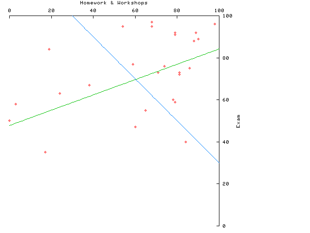
The midterm exam has been graded. The average grade was
73.04. Individual grades have been entered in the FAS
Gradebook. The scatter plot shows the relation between a total of
homework and workshops on the horizontal axis and the exam score on
the vertical. The image also includes a regression line and a line
dividing satisfactory from deficient work to aid in assigning warning
grades. There is also a distribution
of scores (but no attempt to assign letter grades) and
scaled averages (formed my dividing by the maximum possible
score [or base score ] and multiplying by 10) for each
problem. Scaling allows easy comparison of the difficulty of problems
of different weight
Midterm Exam
Distribution
| Range |
Count |
| 88 - 97 |
9 |
| 72 - 84 |
7 |
| 58 - 67 |
5 |
| 35 - 50 |
4 |
|
Problems
| Prob. # |
Scaled
Avg. |
| 1 |
8.94 |
| 2 |
6.00 |
| 3 |
8.34 |
| 4 |
4.54 |
| 5 |
7.40 |
|
More solutions to workshops are available: workshop 5; workshop 6;
workshop 7; workshop 8; workshop 9.
The final exam will also require a calculator and allow the textbook,
but no other resources. Exam questions will be closer to workshop
problems than to the more routine calculations of the homework, but
some computation will appear.
A single summary has been entered in the FAS
Gradebook. The main entry is the numerical score (highest
attained score was less than 400) and the comment shows how it was
built from midterm, homework, workshops, and final. The workshop
grade was divided by 2 to reflect its weight in the course work. The
course grade also appears as part of the comment.
Comments on this page should be sent to: R.T. Bumby
Last updated: December 28, 2003