Math 251 diary, spring 2006
In reverse order: the most recent material is first.
Wednesday, March 1
Yes, a special Wednesday
edition of the course diary. I did not want to fall
further behind in the syllabus, and decided that half a period of
questions about the second derivative test would likely be enough. I
asked the recitation instructors to cover a few more Lagrange
multiplier examples. I did recommend at least two specific examples,
and here are notes on these examples.
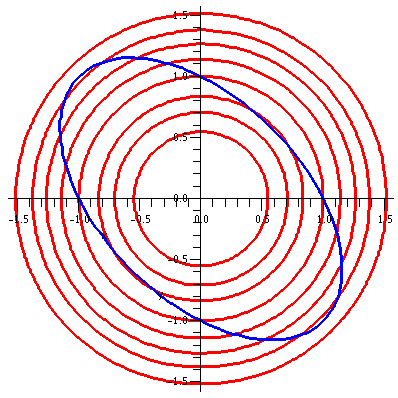 Example #1
Here the constraint is x2+xy+y2=1, and the
function to be maximized, the objective function, is
x2+y2. The picture corresponding to this
situation is shown to the right.
The bigger circles correspond to larger values of the objective
function.
Suppose that T(x,y)=x2+y2 were the temperature
in a thin metal plate with shape the interior of
x2+xy+y2=1, where will the plate be hottest or
coldest? I remind you that in this "heat" language the level curves or
contour lines are called isothermals.
Well, local extrema only occur at critical points, and
only (0,0) is a c.p. That, easily, is the coldest point in the
plate. But where is the hottest point? It must be on the edge, and it
will NOT be a local extremum, but only an extremum for a
constrained maximization. We seek therefore the extrema on the boundary
using Lagrange multipliers.
 Compute the gradients, etc.
Then the multiplier equations and the constraint equation
are:
2x+y=( )(2x)
2y+x=(
 )(2y)
x2+xy+y2=1
Again we can solve with (2x+y)/(2x)=(2y+x)/(2y) so x=+/-y (and
possible special cases of x or y being 0). And so the temperature is
going to be T(x,y)=2 or 2/3 since
x2+xy+y2=1 gives x2=1 or
x2=1/3. There are no solutions with x or y equal 0, because
if one of them is 0 then the other is also 0 (using the two multiplier
equations) and the point (0,0) does not satisfy the third equation.
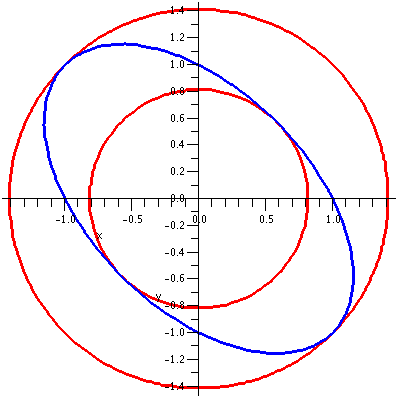
Here is a picture of these special isothermals T(x,y)=2 and
T(x,y)=2/3, and the constraint.
Fan mail for the Lagrange multiplier method
I think it is wonderful that a relatively small amount of
algebraic effort can produce such a lovely geometric result (the
specific circles centered at (0,0) which are also tangent to the
ellipse). This reassures me that things algebraic and geometric both
reflect the same reality.
Proofs, etc.: the dual (?) nature of math
I learned and "liked" Lagrange multipliers in a several variable
calculus course, just as I hope you are. The justification for the
method was more or less what I have shown you. So I knew it was
"true". But I never saw a "proof" of the Lagrange multiplier method
until my second year of grad school. Sigh. It really isn't that
difficult to prove. Maybe I didn't (even as an apprentice professional
mathematician!) feel the need to prove such a lovely idea.
Tuesday, February 28
Proud students volunteered to do some problems at the board. The
instructions were to Find and classify the critical points of
... where classify in this case means see what information the
second derivative test for two variables will provide.
- The function x3+y3-3xy
This function has a saddle at (0,0) and a local min at (1,1.) This is
not obvious and needs to be confirmed by computation.
Ms. Orani and Mr. Nelan and
Ms. Lai and Mr. Bonilla contributed to the solution.
- The function (x/y)+(8/x)-y
This function has a local max at (-4,2). This is
not obvious and needs to be confirmed by computation.
Mr. Boxer and Mr. Ericson and Mr.
Faiwiszewski and Mr. Yen contributed to the solution.
- The function xe-x3+y3
This function has a critical point at (3-1/3,0) and the
second derivative test gives no information. However, if you think of
x as fixed, then we have (Constant)ey3 and this
is an increasing function of y with no minima or maxima. Therefore the
critical point has to be like a saddle, with points close by having
both bigger and smaller values of the function.
Mr. Comito and Ms. Curcio and Mr. Baig and
Mr. Shtabnoy contributed to the solution.
Also we considered (+/-)x4(+/-)y4. Then this
function always has exactly one critical point, (0,0), and (because of
the higher x and y powers) the Hessian, H, of the second derivative
test is always 0. Since depending upon choice of sign, we can have a
strict absolute min or strict absolute max or saddle behavior, we
certainly can't infer anything about the nature of the critical point
when H is 0.
We studied the following problem from 1 variable calculus:
Consider the ellipse x2+5y2=1. Find the
rectangle of largest area inscribed in this ellipse with sides
parallel to the coordinate axes. Of course this turns into: maximize
4xy (the objective function) subject to
x2+5y2=1 (the constraint). Consideration
of the geometry (varying rectangles) suggests that there is indeed a
"biggest" rectangle, somewhere.
How the "heck" does a calc 1 student solve this problem since the
function to be maximized, 4xy, has two variables.
I suggested the following methods of solution:
- Reduction of dimension, simple version
Since
x2+5y2=1, we know that
y=sqrt((1-x2)/5). Then the area is
F(x)=4x·sqrt((1-x2)/5). The domain for this function is
0=<x=<1. General theory from one variable calculus states that
max/min are obtained at end points or critical points. But
F(0)=F(1)=1. So the max is gotten where F'(x)=0. We computed this.
Of course, in a random situation, it may be very difficult to
solve (effectively!) for one of the variables in terms of the other.
- Reduction of dimension by parameterization
We could make an
inspired "guess": try x=cos(theta) and y=sin(theta)/sqrt(5). Then the
pair (x,y) is on the ellipse, and since the max is obtained somewhere
in the first quadrant, we are left with maximizing
4xy=(4/sqrt(5))cos(theta)sin(theta)=(2/sqrt(5))sin(2theta) for theta
between 0 and Pi/2. This can be solved almost "by inspection": just
take theta to be Pi/4. The max value is then 4/sqrt(5). Of course, in
a "random" situation it may be very difficult to get nice
parameterizations.
Now we move from the prosaic
1. like prose, lacking poetic beauty.
2. unromantic; dull; commonplace ("took a prosaic
view of life").
to the more recondite
1. (of a subject or knowledge) abstruse; out of the way; little known.
2. (of an author or style) dealing in abstruse knowledge or allusions;
obscure.
- A weird way to do the problem
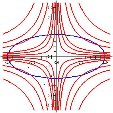
I had Maple sketch some level curves of 4xy, the
objective function, and compare them with the constraint curve
x2+5y2=1. Here is the result of these
Maple commands.
A:=contourplot(x*y,x=-1.1..1.1,y=-1.1..1.1,color=red,
thickness=2,scaling=constrained,grid=[50,50],
contours=[.02,.05,.08,.2,.3,.5,-.02,-.05,-.08,-.2,-.3,-.5]):
B:=implicitplot(x^2+5*y^2=1, x=-4..4,y=-4..4,color=blue,
thickness=2, scaling=constrained, grid=[80,80]):
display({A,B});
The picture is shown to the right. |
 |
A close-up view
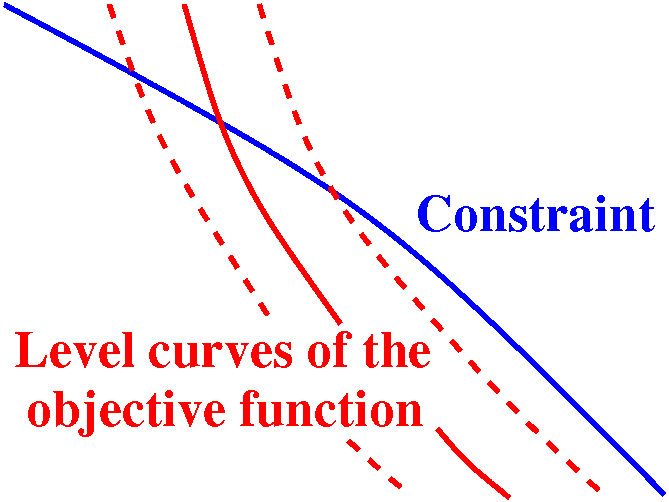
Suppose you consider a level curve of the objective function that
crosses the constraint curve, as shown. One math word which
applies to this situation is that the two curves are
transversal. So we have 4xy=C crossing
x2+5y2=1. What happens if we "wiggle" C a
little bit, so we consider 4xy=C+epsilon and 4xy=C-epsilon. Now it
seems reasonable (4xy is certainly continuous, so its values don't hop
around or break or anything) that these level curves are close to
4xy=C. These level curves must also cross the constraint
curve. That means the function 4xy has values C+epsilon and C-epsilon
on the constraint curve. (The level curves are exactly where that
function takes on its values!) Since there are both larger and smaller
values of 4xy on the constraint curve, C can't be an extreme value
(either max or min) for 4xy on x2+5y2=1.
|
Local picture near a level curve
corresponding to a non-extreme value |
Another close-up view
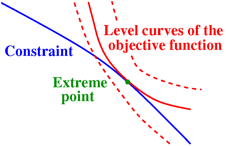
This seems to imply, if you examine the picture closely, that the
largest (and the smallest) values of 4xy will be at points on the
ellipse where the ellipse will be tangent to level curves of the
constraint, x2+5y2=1. If the level curves of the
objective function are not tangent, then we will be able to vary the
values of the constant generating that contour and get bigger and
smaller values of the objective function on the constraint curve.
If the level curves are tangent then the normal vectors of the
constraint curve ( f at that point) and the objective function
( f at that point) and the objective function
( g) at that point will both be perpendicular to the same line (in
three dimensions it would be a tangent plane). These gradient
vectors may not be exactly the same vector, but one of them must be a
scalar multiple of the other. g) at that point will both be perpendicular to the same line (in
three dimensions it would be a tangent plane). These gradient
vectors may not be exactly the same vector, but one of them must be a
scalar multiple of the other.
|
Local picture near a level curve
corresponding to an extreme value |
Now the algebraic side
If f(x,y)=4xy and g(x,y)=x2+5y2=1, then at such
points (extreme values of the objective function on the constraint
curve), there is some real number  so that
  g=
g=
 f (everyone uses this Greek letter) because the tangent
lines are the same, and therefore the normal vectors must be parallel:
one must be a scalar multiple of the other. This one vector equation
in R2 gives two scalar equations, one for each component of
the vectors:
 2x=( )4y
10y=(
 )4x
)4x
This, together
with the constraint equation g(x,y)=x2+5y2=1
gives a system of 3 equations in 3 unknowns. We can solve this by, for
example, solving for  in each
of the first two equations and setting them equal. We need to watch
out for spurious solutions or evasions of solutions. These may occur
when we divide by certain variables. This gave us another way to solve
the maximization problem, a method which is more in the spirit of
several variable calculus. It turns out that this strange idea is
actually quite useful in "real world" problems. The method is called
Lagrange multipliers What kind of
pliers? and is discussed in section 14.8 of the text. The
method is used extensively in economics and in many areas of
engineering.
The first exam returned
I returned the exam. Here is a
discussion of the grades and grading and here are answers. Students who did not do
well should realize that what follows in this course is
more difficult for most people than what we've done. I strongly
suggest that any student with a grade less than 40 carefully consider
withdrawing from the course.
34 of the 140 students who took the exam did not come to the next
class to pick up their graded exams. I take the course seriously.
Therefore I flew across the continent Saturday night to read your
papers and return exams as soon as possible. I tried to grade your work
carefully. Please: you should take your education seriously
also. Unsurprisingly, the average grade of the exams which were not
picked up was substantially lower than the overall course average.
HOMEWORK
Please hand in 14.7: 6, 12 tomorrow in recitation.
Be prepared to discuss problems in 14.7 and to go on in section
14.8.
You will have a
quiz.
Tuesday, February 21
Exam matters
Please have your RU identification with you. There are some review sessions. The lecturer
will not be able to have office hours on Thursday, February 23.
Max/min in several variables
I remarked that that finding maximums and minimums (usually called
together, "extreme values") can be both theoretically and
computationally very difficult. In 251, we "scratch the surface". Some
straightforward definitions are given, and a few techniques are
explored. Mostly we will look at functions of two variables, sometimes
in three, and rarely in more variables. Even in two variables, as I
hope to show you, things can be very different from one variable and
can be computationally very complicated.
Review of 1 variable
I try not to work hard, so I thought maybe a quick review of extreme
value material from 1 variable calculus would be useful. The names of
ideas to recall include these:
maximum, minimum, absolute maximum, absolute minimum, local maximum,
local minimum.
Fermat's fact
What I called "Fermat's fact" was the following wonderful observation
in one-variable calculus:
If f is differentiable at x0
and if f´(x0) is not 0, then f does not have an
extreme value at x0.
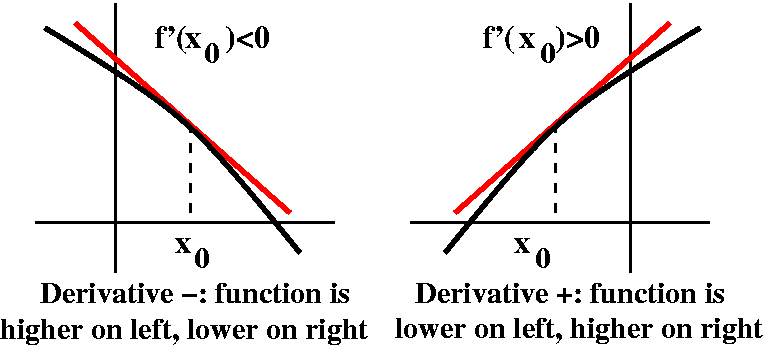
The picture shows a "proof" (well, I hope fairly convincing to a
picture person). If there is a tilt in the tangent line, then there
are both higher and lower values near x0. If x0
is either kind of extreme value (max/min), then we see that
f´(x0) cannot be 0.
Critical number
Therefore the following definition is written.
x0 is a critical number of the function f
if either f is not differentiable at x0 or
f´(x0)=0.
For simplicity in this discussion I'll assume that f is defined in some
interval that has x0 inside it (in the interior).
Consequence
Here is the result which has made calculus famous and earned big bucks:
If f has an extreme value at x0 then x0 is a
critical number of f.
So you can search for extreme values by looking first for critical numbers.
Conversely
I asked if the converse of the preceding statement was true. Maybe you
should have some acquaintance with logic
words. Here I'm asking whether x0 being a critical
number means that the function f must have an extreme value at
x0. The answer is certainly "No." I hope you find the
pictures will be persuasive and/or help your memory.
 By the way, the type of functions illustrated in the first and third
pictures are called piecewise linear. In lots of variables, finding
extreme values of these functions is rather difficult. The problems
are wildly varied, and can deal with topics like scheduling and
allocation. You could begin with an undergrad course to study the
math of these problems (Linear Optimization) and then look into
various aspects of Operations Research or Industrial Engineering.
Identifying ("classifying") the type of critical point
Well, suppose you "have" a critical number. How can we discover if the
function has extreme (max or min) behavior there? I'll make a very
restrictive assumption, which is that the functions
we'll consider will always be differentiable, so corners and jumps and
other very poor local behavior won't occur. Then there are various
observations which can be made, and some will guarantee a (local) max
or a (local) min.
The 68th derivative test
I stated the following result and remarked that almost surely this was
in everyone's calc 1 course:
Theorem Suppose that f´(x0)=0 and f´´(x0)=0 and
f´´´(x0)=0 and f(4)(x0)=0 and ... and
f(67)(x0)=0. (The first 67 derivatives of f at x0 are all 0).
Then
If f(68)(x0)>0, f must have a local max at x0.
If f(68)(x0)<0, f must have a local min at x0.
If f(68)(x0)=0, the 68th derivative text supplies no information.
Huh?
Well, I don't know many calc 1 courses which do teach the
"68th derivative test". Maybe this is because the "test" is
silly, or maybe because the best way to understand why it is true is
to use Taylor's Theorem. I had mentioned way near the beginning of the
course that Taylor's Theorem is a calc 2 result which turns out to be
very useful. Here if we use Taylor's Theorem centered at x0
up to degree 67, we would see something like:
f(x)=f(x0)+lots of
0's+[f(68)(near x0)/68!](x-x0)(68).
Since 68 is even, if the sign of the 68th derivative is
positive, f will have the predicted local min (the graph will look
like a really narrow parabola locally!). And a negative sign gives the
other implication.
I mentioned this absurd "test" so that when you see what happens in,
say, 2 variables, you won't be as horrified or startled as you might
be. The whole process is to decide what algebraic conditions on
derivatives at a critical point can guarantee extreme behavior. The
second derivative test in 1 variable is just the tip of the iceberg
(the snout of the shark?).
Now several variables
Today's word: morass. A neat word, which I didn't make up but which I
always laughed at early in life. It means:
- an entanglement; a disordered situation, esp. one impeding
progress.
- [literary] a bog or marsh.
The max/min situation in more than one variable is much more
complicated. Some examples will be useful.
The simple pictures with simple formulas
In class I presented the pictures initially and then the formulas. I
will do both together here.
| Discussion and formulas | The pictures |
|---|
Min
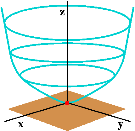
A function defined on all of R2 with a local (and absolute)
minimum is f(x,y)=x2+y2. The graph of this
function is a surface called a paraboloid. It is a nice, smooth
"cup" opening up. Vertical slices through (0,0) are all parabolas
opening up and the contour lines are circles.
The red dot is the critical point and
the brown plane is the tangent plane
at that point (the xy-plane).
|
|
Min
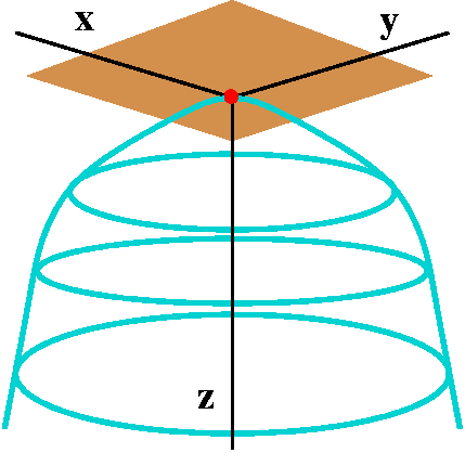
The simplest local and absolute strict maximum is, of course, just the
reflection of the previous example, done with minus signs
algebraically. So here f(x,y)=-x2-y2, and (0,0)
provides a strict maximum. The graph is a paraboloid whose axis of
symmetry is again the z-axis. This graph opens "down".
|
|
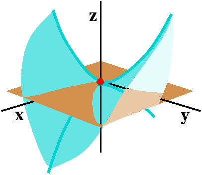
A saddle
The function f(x,y)=-x2+y2 gives a nice example
of a saddle point. The xz-slice (where y=0) shows the curve
z=-x2 and the yz-slice (where x=0) shows
z=y2. Each has a (strict) extreme point at 0. One is a max
and one is a min. Such behavior is called a saddle
point. Perhaps the behavior most similar in one variable calculus
would be that of the function x3 (an inflection point). But
in 2 and more variables the local situation can be much more
complicated.
Here the surface is more complicated, and my picture is certainly not
so good. But the tangent plane and critical point are the same. The
tangent plane cuts through the surface (similar to the way a tangent
line at an inflection point in 1 variable calculus cuts through the
graph of a curve).
|
|
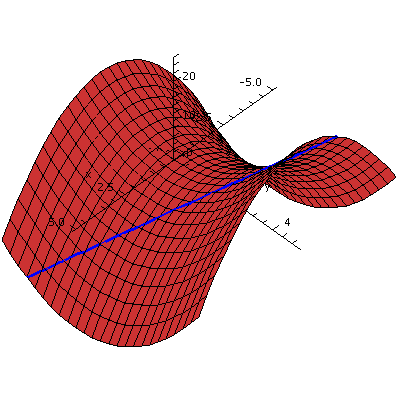 Ridiculous interesting (?) fact
The surface z=-x2+y2 is what's called a ruled
surface. The word 'rule" comes from an older version of English, and
here means "straight line".
Every point on the surface is on a straight line which sits entirely
in the surface. I didn't believe this when I was told it for the first
time, and maybe you don't either. For example, the point (1,2,3) is on
this surface (since 3=-12+22) and the line whose
parametric equation is x=1+t, y=2-t, and z=3-6t goes through that
point and sits entirely on the surface. Such surfaces have
applications in computer graphics.
You can verify algebraically that the line whose parametric equations
gare given above is on the surface, or you can look at the picture to
the right, which shows the saddle together with the line: nearly
silly.
Definition of critical point
Suppose f is a function of n variables. Then f has a critical
point at p in Rn if either  f doesn't exist at p (so
at least one of the first partial derivatives fails to exist) or
 f(p)=0 (the zero vector, remember!).
In this course, almost all the functions we'll consider will be
differentiable. This doesn't mean that non-differentiable functions
)functions with jumps or corners) are not important or interesting in
mathematics and its applications (again: linear optimization, shock
waves in physical phenomena). Just learning to use the tools for higher
dimensional analysis of differentiable functions is a big enough
task.
Suppose z=f(x,y), and f is differentiable. What is the geometric
meaning of "(x0,y0) is a critical point of f"?
Since  f(x0,y0)=0, both of the first partial
derivatives are 0. Therefore z=f(x0,y0) (that
is, z=a constant) is the tangent plane to z=f(x,y) at the point
(x0,y0,f(x0,y0)). The
"flat" plane through the point, parallel to the xy-coordinate plane,
is tangent to the surface. This can be difficult to "see" in a graph,
though.
Using Fermat's fact here
If a point is a local extreme point of some function f in several
variables, and if that function is differentiable at that
point, then all of the first partial derivatives of the function must
be 0 at that point. If that's not true, just "slice" the function at
that point in the direction of the derivative which is not 0. The one
variable Fermat fact implies that the function does not have an
extreme value (max or min) at the point in one variable, and therefore
the function in several variables has both higher and lower values
near the point. Therefore (whew!):
An extreme point must be a critical point.
Our functions will almost always be differentiable, so our functions
will have their extreme values where  f=0.
f=0.
 Monkey saddle
The examples already shown are the standard critical points for
functions of two variables. But there are many, many other kinds of
critical points. The graph z=x3-3xy2 shows one
of them. Again the origin, (0,0), is the only critical point, and the
xy-plane is the tangent plane at the origin. This critical point's
local behavior is up/down repeated three times (at equally spaced
120o angular intervals) if you walk around the
surface in a small circle centered at the origin. The critical point
is called a monkey saddle because, presumably, a monkey could
sit on it with spaces for two legs and a tail to hang down.
Critical points of more than one variable can have many, many
different local pictures, and there has been a great deal of effort
expended trying to understand them.
Two book problems
There are two amazing and disconcerting problems in section 14.7. At
least, to me these problems are both amazing ("surprise greatly;
overwhelm with wonder" -- well, at least the first) and disconcerting
("disturb the composure of; agitate; fluster" -- certainly they show
me I don't understand too well what can happen in "space").
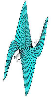
Problem #35, section 14.7
The function
f(x,y)=-(x2-1)2-(x2y-x-1)2
is given. This is not the world's most horrible function. It is "only"
a polynomial of degree 6. First, the text asserts that this function
has two critical points. We can check that easily:
Hey! I was going to do this "by hand" when I realized that I could
have a friend (?) do it. So here:
> f:=-(x^2-1)^2-(x^2*y-x-1)^2;
                               2     2     2           2
                       f := -(x  - 1)  - (x  y - x - 1)
> solve({diff(f,x),diff(f,y)});
                        {x = 1, y = 2}, {x = -1, y = 0}
Yup, two critical points. Below are two very local pictures of
the graphs near the critical points.
 The pictures certainly shouldn't be convincing evidence, but they do
support the textbook's assertion that the function has local minimums
at both critical points! (We can verify this assertion with the second
derivative test to be stated later.)
Why do I find this disconcerting? Well,
imagine we walk from one peak to another (shown to the right, the
blue "trail").
  Shouldn't we somehow pass through a saddle? Well, in
fact, no, we don't need to: maybe the lowest point on the blue trail
is not a critical point -- the tangent plane to the surface at that
point may be tilted. In this example, the tangent plane is
always tilted at every point except the two peaks.
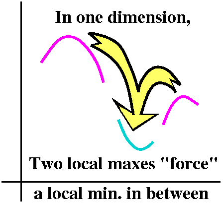
The situation in 1 variable calculus is considerably different.
If I
have two local maxes (and, yeah, if the function is continuous,
differentiable, etc.: nice) then there must be a local min between
them.
Problem #36, section 14.7
Here f(x,y)=3xey-x3-e3y. I think even
I showed that this has one critical point. My friend replies:
> f:=3*x*exp(y)-x^3-exp(3*y);
                                           3
                        f := 3 x exp(y) - x  - exp(3 y)

> solve({diff(f,x),diff(f,y)});
                               2                                 2
 {x = 1, y = 0}, {x = RootOf(_Z  + _Z + 1), y = ln(-1 - RootOf(_Z  + _Z + 1))}
Since I know that z2+z+1 has no real roots (the
discriminant is 12-4·1·1=-3<0) this
function has exactly one critical point. And the formula for
the function isn't really that horrible, either.
The left graph below is a local picture of the critical point. This
seems to convincingly support the textbook's assertion that (1,0) is a
local strict maximum of the function. (We can verify this assertion with the second
derivative test to be stated later.) In the graph on the right,
x goes from -5 to 5 and y varies just between -.05 and .05: therefore
y is just about 0, and 3xey-x3-e3y is
just about 3x-x3-1. Certainly this shows that the function
has no absolute max or min.
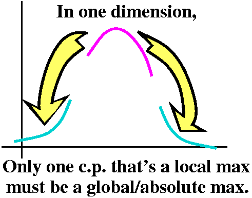
The situation in 1 variable calculus is considerably different.
Suppose we have a function defined on all of the real numbers (o.k., a
differentiable which has exactly one critical point and that
critical point is a local maximum. Then that local maximum is a
global, absolute maximum for the function. What the heck is
happening in several variables? I just don't understand, really
understand.
Now a second derivative test in two variables
There's one second derivative test which is usually "given" to
students in a third semester calculus course. It is a bit
complicated. The test essentially results from computing the second
directional derivative at the critical point and seeing how to ensure
that this result is always positive (or always negative or ...). That
together with results from one variable calculus (on concavity) will
insure some kinds of local behavior near the critical point.
Diary entry in progress! More to
come.
Using the chain rule
and the chain rule more
Now the transition to something
The statement of the second derivative test
Hessian: http://en.wikipedia.org/wiki/Hessian_matrix
QotD
Diary entry in progress! More to
come.
Friday, February 17
 sloth laziness or indolence; reluctance
to make an effort.
(Also an animal, about which is written:
"... Sloths move
only when necessary and then very slowly: they
have about
half as much muscle tissue as other animals of similar
weight.")
Today's lecture discusses the most important single application of the
chain rule, and maybe the most important single idea in vector
differential calculus. I'll introduce it with a silly but still almost
reasonable "story".
The spaceship in a nebula
My online dictionary states that a nebula is "a cloud of gas
and dust, sometimes glowing and sometimes appearing as a dark
silhouette against other glowing matter." So we could pilot a
spaceship through a nebula. We might be concerned about the physical
effects of the nebula, for example, the temperature. I'll assume that
the spaceship measures temperature at the tip of its front. A point in
the nebula will be located with rectangular coordinates, (x,y,z). The
temperature at that point will be T(x,y,z). The rocket will fly a path
so that at time t its location will be <x(t),y(t),z(t)>.
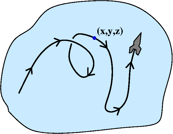 From this we can see that the temperature measured at the rocket at
time t is T(t)=T(x(t),y(t),z(t)), and this is a composition. First we
find out where the spaceship is at time t, and then we compute the
temperature at that point.
Computing dT/dt
Well, the chain rule applies, so
dT 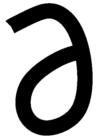 T dx
T dx  T dy
T dy  T dz
-- = --- -- + --- -- + --- --
dt
  x dt
x dt  y dt
y dt  z dt
z dt
Recognition
Now the luck and glory is recognizing that the mess on the righthand
side is a dot product. In fact, look:
dT /  T
T  T
T  T \ / dx dy dz \
-- = --- , --- , --- · -- , -- , --
dt \
  x
x  x
x  x / \ dt dt dt /
Left Right
There are certainly many ways to organize this as a dot product, but
this way turns out to give some insights that amaze me.
Right
The vector on the right-hand side is one we've looked at when
discussing curves. It is the derivative of r(t), the position vector,
so it is v(t), the velocity vector. This vector deals with the
spaceship and its motion.
Left
This vector seems to be "new": it is the vector of all the first
partial derivatives of T in order. This is called the gradient of
T and is frequently written  T. The upside-down triangle (or upside down
 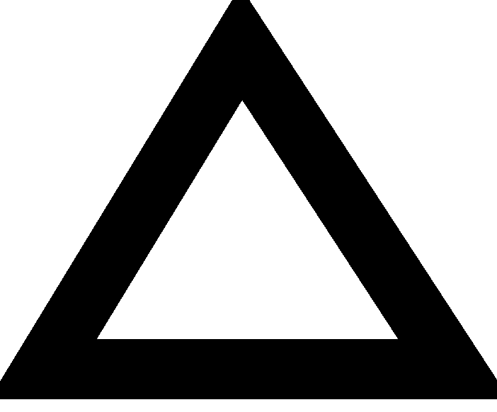 ) is
sometimes called "del". This vector can be computed only from the
nebula information.
So we have separated ("decoupled", where one definition of "decouple"
is "disconnect or separate") the nebula and the spaceship. The nebula
information is  T and the spaceship information is v(t).
Now I tried to make a sequence of observations which might help people
understand the actual excitement I feel thinking about gradient.
Observation 1
Let's imagine two spaceship trips through the nebula. Now these
trips (voyages?) may be completely different except that at the
time the two spaceships pass through the point (x,y,z), the
spaceships have the same velocity vectors: that is, the spaceships are
heading in the same direction and at the same speed. Their v(t)'s are
the same. Then the rate of change of the temperature,
dT/dt, that the two spaceships measure is exactly the
same.
I asked students if they could deduce this from the physical and
geometric aspects of the "scenario". I don't think I can. As a math
fact goes, this is nearly obvious: since the v(t)'s are the same, the
right-hand side doesn't change, and the nebula's temperature function
is the same, so the left-hand vector ( T) doesn't change. Therefore
the dot product, which computes dT/dt, is the same. But ... but
... what the heck ... can you "see" this physically? This is not the
temperature at the point, but the rate of change of the
temperature: the rate of change is the same if the velocity vectors
are the same.
Observation 2
Now r´(t)=v(t), the velocity vector. It is the same as
(ds/dt)T(t) where ds/dt is the speed and T(t) is the unit tangent
vector. In the formula  T·r´(t) the ds/dt effect just "filters
out" of the dot product. If you travel twice as fast on the same path,
then the rate of change of the temperature with respect to time is
just doubled. So this is easy to understand. But, as several students
in both lectures observed, the more subtle aspect is what happens as
the direction changes.
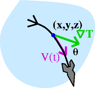 Observation 3
Here I will suppose that ds/dt=1 for simplicity. Also in order to keep
my notation sane (how many uses of T can I have in the same problem?)
I will replace the unit tangent vector by u, for unit
vector. Then what can we say about  T·r´(t)? It is
(ds/dt)
 T·u, or just (since I'm assuming unit speed)
 T·u. But, hey, the dot product is also
|
 T| |u|cos(theta). Since cos(theta) is between -1 and +1, I
now know that dT/dt is between -|
 T| and +|
 T|.
T|.
How could we choose u so that dT/dt is largest? We need to make
cos(theta) equal to +1. Therefore we need theta to be 0, and u should
be a unit vector in the direction of  T. That is, choose u to be
 T/|
T/| T|. To make the rate of change as much negative as possible,
choose u to be -
 T/|
T/| T|, and then dT/dt will be -|
 T|.
T|.
An example (?)
Students' patience for abstraction began to wear out. So I computed an
example.
If T(x,y,z)=x2eyz-5z3 then since
 T=<
T=< T/
T/ x,
x, T/
T/ y,
y, T/
T/ z>, we compute:
 T=<2xeyz-5z3,x2eyz-5z3(z),x2eyz-5z3(y-15z2)>
As far as I know this function and this computation has no great or special
"meaning".
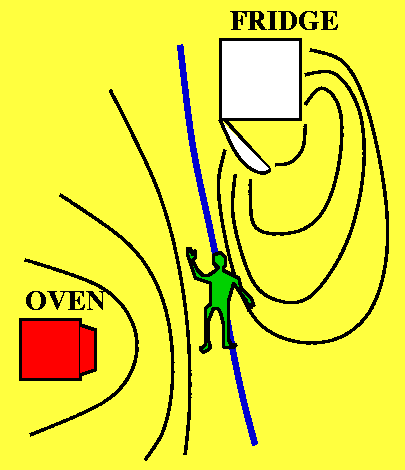 A better example (!)
Im my kitchen I have just finished backing my famous chocolate brownie
pie and I left the oven door slightly open. Also I managed to forget
to close the refrigerator. As a result, the contour lines of
temperature could like what is shown to the right. In what direction
should I go (I am the little green man in the picture!) to most
rapidly increase the temperature? In the direction of the gradient,
which will point towards the oven. I will most rapidly decrease the
temperature by traveling in the opposite direction, towards the source
of the cold.
Observation 4
I could imagine that spaceship travels through the nebula on an
isothermal surface. An isothermal is a collection of points
where the temperature is all the same. We have seen this already:
T(x,y,z)=C is a level surface (dimension 3) or level curve (dimension
2) or a contour {surface|curve}. But if the spaceship travels on such
a surface, then the rate of change of the temperature must be 0. But
then  T·v=0. This means that the velocity vector is perpendicular
to the gradient. But then in turn this means that the gradient vector
is perpendicular to the level surface, and it is perpendicular to the
tangent plane of the level surface. In the kitchen, I would walk
perpendicular to the contour lines to increase or decrease
temperature most rapidly. I would walk along the contour lines if I
wanted no rate of change of temperature.
Back to the example
Let me look more closely at the example with
T(x,y,z)=x2eyz-5z3
when x=3 and y=2 and z=1. Well, T(3,2,1)=9e-3. And
 T=<2xeyz-5z3,x2eyz-5z3(z),x2eyz-5z3(y-15z2)>
becomes
 T(3,2,1)=<6e-3,9e-3(1),9e-3(-13)>=<6e-3,9e-3(z),-117e-3>
Now forget all that, and solve the following
geometric problem:
What is the equation of a line tangent to the surface
x2eyz-5z3=9e-3 at the
point (3,2,1)?
This could be, indeed, I claim, this is a hard problem. But if
we now disobey my urging ("forget all that") I can tell you that
 T(3,2,1) is perpendicular to the surface and to its tangent plane
at (3,2,1). So I can write the answer, since I know a point and a
normal vector to the plane requested:
6e-3(x-3)+9e-3(y-2)+-117e-3(z-1)=0.
I think that solving such a problem so efficiently is really remarkable.
Topographic maps
A topographic map shows contour lines. Frequently while hiking people
mind want to find the most direct route to the "top" (a mountain peak)
or to the "bottom" (a creek?). They know by experience that the most
direct route, only looking at the map, that is, only the geometry of
the situation, would be to walk as nearly as possibly perpendicular to
the contour lines.
This can be adapted into computational strategies for finding
maxes and mins. If you can readily compute your function's gradient,
then find maximums by going in the direction of the gradient. This is
hill climbing. Find minimums by going opposite the direction
of the gradient. This is the method of steepest descent. Of
course these computational ideas don't always work, and there are a
great deal of implementational matters to worry about, but the general
strategy is valuable.
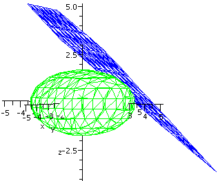 Ellipsoid
Here's a neater example. Consider the ellipsoid (egg)
x2+2y2+3z2=9. The point
(2,1,1) is on this ellipsoid. What is the equation of a plane tangent
to the ellipsoid at (2,1,1)? Well, the gradient of the function
x2+2y2+3z2 is
<2x,4y,6z> and at (2,1,1) this is <4,4,6>. The equation of
the tangent plane is 4(x-2)+4(y-1)+6(z-1)=0.
To the right is a Maple picture made by the commands which
follow. I hope that the picture helps to convince you that the plane
is the tangent plane.
A:=implicitplot3d(x^2+2*y^2+3*z^2=9,x=-5..5,y=-5..5,z=-5..5,grid=[20,20,20],
axes=normal,labels=[x,y,z],color=green,style=hidden);
B:=implicitplot3d(4*(x-2)_4*(y-1)+6*(z-1)=0,x=-5..5,y=-5..5,z=-5..5,axes=normal,
labels=[x,y,z],color=green,style=hidden);
display({A,B};
Directional derivative
If u is a unit vector, then the directional derivative of T at (x,y,z)
in the direction u is the rate of change of T at unit speed in the
direction u (at the point). The textbook's notation for this is
DuT(x,y,z) and the preceding discussion should convince you
that the directional derivative's value is  T(x,y,z)·u.
more notation, more words ... this is so
terrific!!! (so academic)
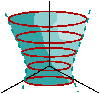
QotD
I asked people to look at a hyperboloid, a surface given by the
equation x2+y2-z2=12. The point
(3,2,1) is on this surface. Since
x2+y2=12+z2
I know that slices with z fixed are circles. The slice on the xy,plane
is a circle with center the origin and radius sqrt(12). As z
increases, the slice is still a circle with center (0,0) (on the
z-axis) but the radius is increasing and is
sqrt(12+z2). The picture to the right is supposed to show
some representative circles and "suggest" part of the surface to you.
The Maple command
implicitplot3d(x^2+y^2-z^2=12,x=-5..5,y=-5..5,z=-8..8,grid=[20,20,20],
axes=normal,labels=[x,y,z],color=green,style=hidden);
will get you a nice picture which you can rotate and examine.
I asked for the equation of a plane tangent to this hyperboloid at
(3,2,1) and also for the three parametric equations of a normal line
to the hyperboloid at (3,2,1). I tried to emphasize that almost no
computation would be needed. Since the gradient of x^2+y^2-z^2 is
<2x,2y,-2z> we can just evaluate this at (3,2,1) and get
<6,4,-2> and this vector is normal to the hyperboloid at
(3,2,1). Here are the answers:
The tangent plane: 6(x-3)+4(y-2)-2(z-1)=0
The normal line:
x=3+6t
y=2+4t
z=1-2t
HOMEWORK
- Do the workshop problem.
- Look at the formula sheet and the review problems. Please
send in solutions! Sincere statement: I would very much like students
to do well on the exam, and for that to occur, students should practice. Most of the exam will
cover material which has been emphasized in lectures and in homework.
- Do problems in 14.5 and 14.6. The content is quite important.
- There are no textbook problems due in recitation Wednesday
(only the workshop problem!).
- You may try the spade suit problem from the handout. The answer is
available here.
Tuesday, February 14
Flip and differentiate
Just for fun (really!) I began the class by discussing this situation:
Suppose f(x,y)=(sin(y4)x-7)3. Then I flip a (fair) coin. If it lands
"heads", I  /
/ x this function. If the coin shows "tails", I
  /
/ y
the function. What's going to happen? I asked students to speculate
about this. Almost everything that students said was correct. I
sometimes tried to distract people from the real question by making
interesting and true assertions. For example, I remarked that
 100f/
100f/ y100 yields a mess with 342 terms. And
200 y derivatives gives an algebraic mess with 680 terms. These
computations were not done by hand, but with Maple. The
expressions begin to swell (get larger and larger). I asked
students if they thought that this sort of growth would be likely
under the conditions of the experiment. Students kept remarking about
 /
/ x and I kept "distracting" with facts about
  /
/ y. Well, here's
a result that some students made me write:
Clairaut's Theorem (equality of "mixed" partial derivatives)
Suppose f(x,y) is a function of two variables, and the mixed partial
derivatives fxy and fyx both exist and are both
continuous. Then these mixed partial derivatives must be the same.
Certainly in Math 251, the hypotheses of the theorem will be
satisfied. There are examples (similar in nature to the bizarre
functions previously given) where things aren't the same. But in this
course, the mixed partials will be continuous and therefore will
agree. The verification of this result is in the textbook and uses the
Mean Value Theorem of 1 variable calculus. As I said, this result will
apply to the functions we will meet in 251. The result implies, for
example, that if we look at the "crowd" of all the possible third
partial derivatives of a function of two variables:
fxxx fxxy fxyx fyxx fxyy fyxy fyyx fyyy
it may seem that there are eight possibilities. But due to Clairaut,
there are only these four:
fxxx fxxy fxyy fyyy
The effect of the "concentration" gets even stronger as the number of
derivatives increases.
But what happens?
How does Clairaut influence my original question? Again, I was perhaps
not the most helpful person in leading the discussion, but eventually
the most relevant fact appeared. The function
f(x,y)=(sin(y4)x-7)3 is a cubic (degree 3) polynomial in x. That is, it can be written as
Stuff0x0+Stuff1x1+Stuff2x2+Stuff3x3
where each of the "Stuff" terms is some function of y alone. An x
derivative,  /
/ x, lowers the degree in x. And four x derivatives
will leave us with 0. If you toss a coin a large number of times, it
is overwhelmingly likely that there will be at least 4 heads, and
therefore, in the differentiation choices, at least 4 x
derivatives. So since we can reorder these mixed partials in any way
we want, we could put those four derivatives first. And the result
will be 0. So, almost surely, if we toss a coin many times, and follow
the directed sequence of derivatives, the result will be 0.
The handout
Then with the help of a student volunteer (frowning at a student
creates a volunteer!), each student received a copy of data about some functions.
Do we understand the handout?
I remarked that I used unusual variable names and some new
notation. The first table on the handout. f and g are declared to be
differentiable functions of two variables.
  M     N  f(M,N) D1f(M,N) D2f(M,N)  g(M,N) D1g(M,N) D2g(M,N)
 -1    -2     6      4        0         3      8       1
 -1     2     2     -2        1        -5      7       6
  1    -1    -2     -5        4        -2      9       4
  1     2     5     -7        6        -1     -2       7
  2     1     0     -1       -2        -3      7       4
So M and N specify inputs to the functions f and g. Therefore f's
value when, say, M=1 and N=2, is 5: f(1,2)=5. What are the
D1 and D2 columns? This is another notation for
partial derivatives, notation which some people prefer when there
might be confusion about how the variables are named. D1
would refer to the partial derivative with respect to the first
variable (frequently we have called this x) and D2 is the
second variable (usually called y). Therefore in more traditional
notation,  f/
f/ x(1,2)=-7 and
  g/
g/ y(-1,2)=6.
The second table on the handout referred to values to two
differentiable functions of one variable.
  V  h(V)  h´(v)  k(V)  k´(v)
 -2   5     2      3     5
  0   0     2     -2     7
  1   1     3      2    -1
  2  -1     4      4    -2
Maybe this table (in spite of the choice of variable name: V!) is a
bit easier to understand. The value of the function k at input 1 is2, and k's derivative at 1 has value -1. Also, h(0)=2 and h´(0)=3.
Doing the problems
A sequence of four problems were given. Let's try them.
Club suit
If S(t)=h(k(t)), compute S(1) and S´(1).
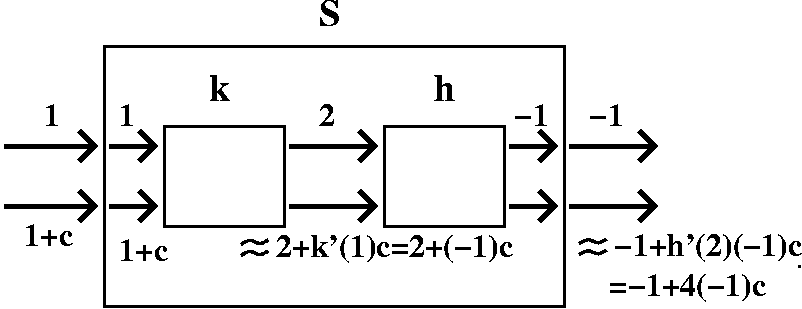
This is one variable calculus. But let me try to think about it a bit
first:
Thinking about it
I can think about the function S as a sort of box, which takes inputs
and processes them in some fashion, and produces outputs. The S box
also has some internal structure. The input first is sent to box
representing the k function, and then the output from that (sub?)box
is sent to the h function. If we follow through (using values from the
second table) we can see that 1 "changes" to 2 and then to -1.
What about the derivative? The derivative is a multiplier of a
tiny change in the input. It signals the first order change in the
output compared to the input. In the case of S, if we "kick" the input
by c (think of c as a small number) then 1+c is fed into the k
box. The output will be approximately (neglecting H.O.T., higher order
terms) 2 (the old output) +k´(1)c, which is 2+(-1)c. Now feed in
2+(-1)c. If c is small, (-1)c will be small. The output from the h box
will be -1 (the old output, what h "does" to 2, plus a change. The
first order part of the change will be a proportionality constant,
h´(2), multiplying the kick that is passed to the h box. The kick
passed to the h box is (-1)c, so the compounded effect is that h's new
output (approximately, first order) is -1 (the old value of h's
output) plus h´(2)(-1)c=4(-1)c.
Now go "up" a logical level. The input, 1, to S was kicked to 1+c. The
S output, to first order, is -1 (the old output) plus
4(-1)c. Therefore the derivative of the S box at 1 is 4(-1), since the
derivative is the multiplier of the kick.
The diagram below is supposed to be visual "support" of the preceding
discussion.
A formula
If S(t)=h(k(t)), the one variable chain rule states that
S´(t)=h´(k(t))k´(t), so S´(1)=h´(k(1))k´(1)=4(-1).
Formulas are good!
Diamond suit
If W(t)=f(h(t),k(t)), compute W(1) and W´(1).
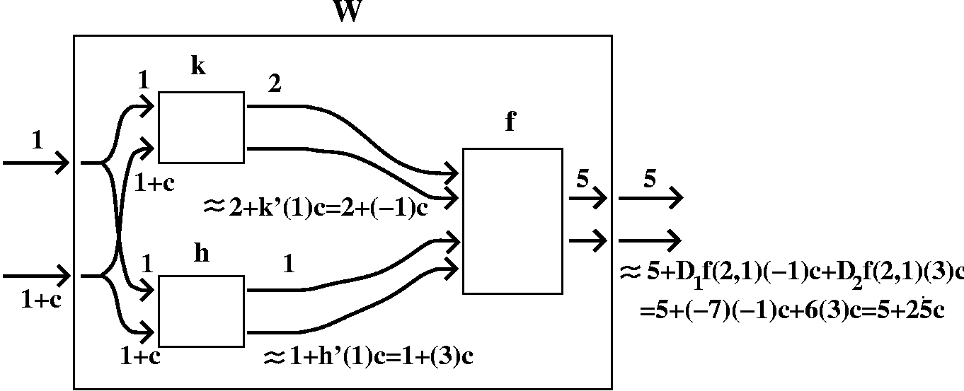
Thinking about it
Now the W box has a different structure. The input is split
(bifurcated -- what's the point of being in an academic environment if
a silly, uncommon word isn't used in place of one that would be
understood!) into two, and each is fed separately into h and k
boxes. The outputs, now in order, are carefully put into f. The output
from the f box is then pushed outside as the value of W.
To compute W(1), we find h(1)=1 and k(1)=2, and then compute
f(1,2)=5. Easy (?)..
What about the derivative? Suppose we kick 1 to 1+c. The response of
the one variable boxes, h and k, should not be difficult to
understand: the outputs, linearized, are 2+k´(1)c=2+(-1)c and
1+h´(1)c=-1+3c, respectively. It is important to remember which
output is which! Now feed this into f. The multiplier for
perturbations in the first variable is D1f(2,1), so the
effect of the change in the first variable adds on
D1f(2,1)(-1)c to the output. The second variable
contributes in proportion to its perturbation, with the constant of
proportionality being D2f(1,2), so D2f(1,2)(3)c
gets added on. If we look up the numbers and do arithmetic, we can see
that the total (linearized) effect (neglecting higher order errors!)
is 5 (the old output) plus 25c. Therefore the output of the W box
seems to indicate that the derivative is 25.
A formula
O.k., if W(t)=f(h(t),k(t)), we will label the variables in f: the
first variable is x and the second variable is y. Then we follow
through the changes and use the chain rule:
W´(t)=( f/
f/ x)h´(t)+(
 f/
f/ y)k´(t).
This is a fine result, but if we need to evaluate it, we'd better
remember that
W´(t)=( f/
f/ x)(h(t),k(t))h´(t)+(
 f/
f/ y)(h(t),k(t))k´(t).
and now you should see the numbers that appeared above.
Heart suit
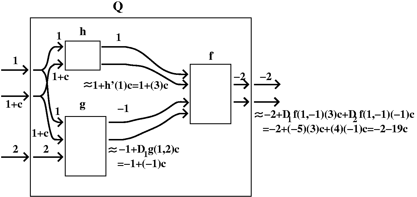
If Q(x,y)=f(h(x),g(x,y)), compute Q(1,2) and  D/
D/ x(1,2) and
  D/
D/ y(1,2).
Thinking about it
Certainly Q(1,2)=f(h(1),g(1,2))=f(1,-1)=-2: easy enough. Now to get
the derivative with respect to "x", the first variable, let's
perturb or kick 1 to 1+c. The effect filters through h as
(linearized!) 1+h´(1)c which is 1+3c. If we kick 1 in g but hold the
second variable constant at 2, then the output, to first order, is -1
(the old output) plus D1g(1,2)c. This is -1+(-1)c.
Now the input to f is, in order, 1+3c and -1+(-1)c. There are changes
to both variables. So we need to use a linear approximation in both
variables. The output from f (which is what is reported as the output
from Q) will be
-2+D1f(1,-1)(3)c+Df(1,-1)(-1)c=-2+(-5)(3)c+4(-1)c=-2+(-19)c. Therefore
the proportionality factor is -19, and this is the requested
 Q/
Q/ x(1,2).
A formula
So if Q(x,y)=f(h(x),g(x,y)), then I think that
 Q/
Q/ x=(
x=( f/
f/ x)h´(x)+(
 f/
f/ y)(
y)( g/
g/ x). There's still the question about how to get values, and in fact, in more detail, this chain rule reads:
 Q/
Q/ x(x,y)=(
 f/
f/ x)(h(x),g(x,y))h´(x)+(
 f/
f/ y)(h(x),g(x,y))(
 g/
g/ x)(x,y).
If we want the y derivative, then we could compute this:
 Q/
Q/ y(x,y)=0h´(x)+(
 f/
f/ y)(h(x),g(x,y))(
 g/
g/ y)(x,y).
The 0 is there because there is no y involvement in the
first variable of Q. Now insert x=1 and y=2, and read off from the
information given that the value is 4·7=28.
This is all horrible. I will admit to you that I usually try to use
formulas and only rarely (like most other human beings) try
thinking. But sometimes thinking is needed. For example, those who
like formulas might contemplate this task:
What is the partial derivative with respect to x of
f(h(x),g(y,x))? Notice that I "swapped" the variables in g. I think
the partial derivative with respect to x will be
0h´(x)+( f/
f/ y)(h(x),g(y,x))(
 g/
g/ x)(y,x). Some people might find this notation very
objectionable: look, two y derivatives multiplied are one x derivative!
ODE's
I solved an ordinary differential equation:
Find all solutions of d2y/dx2=x5
This is certainly rather simple, and just two antidifferentiations
gets the following answer: y=(1/42)x7+Cx+D where C and D
are any real constants. So the "family" or collection of solutions of
this ODE is a two-(real)parameter family of functions.
A simple PDE
Here I sort of went backwards (in fact, the going forwards is much
more difficult!). I started with a differentiable function of one
variable, which I called f. Then I looked at this function of two
variables, F(x,y)=f(x2+y3) (slightly different
from what I did in class -- I think this is better because there isn't
symmetry in x and y which maybe is distracting). Then
 F/
F/ x=f´(x2+y3)2x and
 F/
F/ y=f´(x2+y3)3y2
from chain rule arguments similar to what we just did. But then:
(3y2 F/
F/ x=(3y2)f´(x2+y3)2x and
(2x)
 F/
F/ y=(2x)f´(x2+y3)3y2
so "clearly" F(x,y)=f(x2+y3) is a solution of
the partial differential equation
(3y2 F/
F/ x-(2x)
 F/
F/ y=0.
y=0.
So we now have a family of solutions of this PDE. The solutions
include
sin(x2+y3) and
ex2+y3 and
tanh(x2+y3) (well, no one asked, but that's
hyperbolic tangent which is interesting in some fluid flow
problems). PDE's may have lots and lots of solutions. As I mentioned
above, what I've just done is a classroom example. So if you came up
to me with a PDE modeling some "real" phenomenon, I may not be able to
go backwards too easily and get a family of solutions described so
simply.
Implicit functions, two dimensions
Here's another application of the several variable chain rule. Again,
return to a 1 variable calculus situation:
Suppose F(x,y) is a differentiable function of 2 variables, and the
equation F(x,y)=0 defines y implicitly as a function of x. What
is dy/dx in terms of F and "things" related to F?
So take the equation F(x,y)=0 and d/dx this equation. The right-hand
side is 0, and the left gives you:
 F/
F/ x(dx/dx)+
 F/
F/ y(dy/dx)
by the chain rule.
Certainly dx/dx is 1, and dy/dx is what we want, so we can "solve" for
it in the equation  F/
F/ x+
x+ F/
F/ y(dy/dx)=0. This means:
A formula!
dy  F/
F/ x
-- = - ------
dx
  F/
F/ y
y
Example
I think an example is needed here before we go on. Let's look at:
Calc 1 problem: find dy/dx if
y3-7xy2+4x5-6=0.
Calc 1 solution to Calc 1 problem We d/dx everything, being careful
to remember that y=y(x) mysteriously. Then:
3y2y´(x)-7y2-(7x)2yy´(x)+20x4=0,
and now we solve for y´(x). We get:
y´(x)(3y2-(7x)2)-7y2+20x4=0 so that
y´(x)=-(-7y2+20x4)/(3y2-(7x)2).
New technology (?) solution to Calc 1 problem We will use the
formula above. Here F(x,y)=y3-7xy2+4x5-6
so that
 F/
F/ x=-7y2+20x4 and
 F/
F/ y=3y2-(7x)2y+0 and the formula gives
dy/dx=-( F/
F/ x)/(
x)/( F/
F/ y)=-(-7y2+20x4)/(3y2-(7x)2y+0)
which is of course the same answer! And you can look at see the same
pieces occurring, so the world is not so crazy.
The darn formula, though, is a bit mysterious. If you try to
understand the form (?) of the formula, the  x and
x and  y might seem in
the wrong place and there might be an extra minus sign ... and ... and
... the notation is terrible!
P and V and T
I asked if people knew about gas laws. For a gas, there are the
quantities P (pressure) and V (volume) and T (temperature). A gas
law might be a function of three variables which relates these
quantities:
G(V,P,T)=0.
If we assume that the function is differentiable and that each one of
the quantities is implicitly defined as a function of the other two by
the function, something funny happens. Let me show you.
Suppose that G(V,P,T)=0 implicitly defines V as a function of P and
T. Let's compute  V/
V/ P. Here T is constant, and sometimes in
thermodynamics the quantity is called (
 V/
V/ P)T just to
remind people that T is constant. We will
  /
/ V the equation
G(V,P,T)=0.
I use the chain rule, and the result is:
( G/
G/ V)(
V)( V/
V/ P)+(
P)+( G/
G/ P)(
P)( P/
P/ P)+(
P)+( G/
G/ T)(
T)( T/
T/ P)=0.
P)=0.
But  P/
P/ P must be 1 (the derivative of something with respect to
itself) and
  T/
T/ P must be 0 (because T is constant!). Therefore we
can solve for
  P/
P/ V just as we got dy/dx before and get:
 V/
V/ P=-(
P=-( G/
G/ P)/(
P)/( G/
G/ V).
V).
So far so good. But in fact we can find other partials in a similar
way:
 P/
P/ T=-(
T=-( G/
G/ T)/(
T)/( G/
G/ P)
P)
 T/
T/ V=-(
V=-( G/
G/ V)/(
V)/( G/
G/ V).
Now clearly (NOT AT ALL
CLEARLY!):
( V/
V/ P)T(
P)T( P/
P/ T)V(
T)V( T/
T/ V)P=-1
because when we multiply all these expressions together the fractions
all cancel and we are left with -1. Why is this true physically
and what does it mean? Take physical chemistry, take thermo, etc., and
find out (and maybe report back some time to me, please).
QotD (should have been!)
I wanted to ask people to compute the Spade suit problem. If
you would like to try it on your own, here is the answer.
Formulas, reviews, etc. for the first exam
There's an exam a week from Friday. Please look at the formula sheet
and let me know about errors. Please look at the review problems, and
contribute generously to the welfare of Math
251 by sending
me a solution to the problem whose initial is your last name's
initial, if no solution is yet shown.
HOMEWORK
Sane human beings would do the assigned workshop problem, work on
textbook problems, look at the review material and formula sheet, and
maybe even glance at the next section (the last section to be tested
on the exam).
Friday, February 10
Thundersnow
Along with the blizzard warnings we've had this morning, there has
also been a notification of possible thundersnow, which can be
defined as "A heavy snowstorm with lightning and thunder, or a
lightning discharge during wintry weather." I will listen and look for
this eagerly.
Nuclear magnetic resonance (NMR)
NMR
is a way of investigating the structure of molecules, relying on the
spin of protons and how this spin changes in high magnetic and
electric fields. Several "antiques" (objects 10 years old!) were
exhibited in class. These were contour plots, outputs of NMR
experiments. The lecturer believes students should be aware that real
data can be much more complicated than the examples likely to be seen
in this course!
Limits, 1 dimension
Here we've got a function of one variable, and we want to define and
understand limx-->af(x)=L. The actual definition,
frequently stated but rarely stressed in calc 1 classes, is the
following: (and, yes, the Greek letters epsilon and  are almost
always used)
Given any epsilon>0, there is some  >0 so that if
0<|x-a|< >0 so that if
0<|x-a|< , then |f(x)-L|<epsilon. , then |f(x)-L|<epsilon.
|
One way to possibly understand this is uses the model of a "function
box" as I did in class: a box labeled "f" which has input and
output. In this model, the epsilon is an output tolerance. We'd like
our outputs to be within epsilon of the ideal output (for this
problem) L. Then the limit definition states that there is some input
tolerance,  , which when applied to stuff going into the machine
(only allowing inputs within
  ) then the output tolerance will be
satisfied. The definition itself may be difficult to understand for
several reasons. First, it is a complicated logical statement, Second,
it provides no structure for computing or even estimating
  when
actually given an epsilon. To me, this is a bit distressing. But some
understanding of the input/output model and its approximation
properties is fine right now.
Limits, 2 dimensions
We looked at several examples last time which were not continuous and
did not have limits at (0,0). Let me show you the actual mathematical
definition of lim<x,y>--><a,b>f(x,y)=L. It is
very analogous to the 1 dimensional definition quoted above:
Given any epsilon>0, there is some  >0 so that if
0<|<x,y>--><a,b>|< >0 so that if
0<|<x,y>--><a,b>|< , then |f(x,y)-L|<epsilon. , then |f(x,y)-L|<epsilon.
|
Again the epsilon and  are output and input tolerances,
respectively. The interesting feature to me is
|<x,y>-<a,b>|. This means the distance from <x,y>
to the point <a,b>. This is distance in any direction, along any
path. The examples we saw last time only considered approaches to
<a,b> along straight line segments. This turns out not to be
enough. You've got to allow any paths, and, in fact, allow
consideration of all points close to <a,b> (a sort of blob
completely surrounding <a,b>). I think this makes limits much
more "strict" in several dimensions.
Derivative, 1 dimension
What does f´(x)=Q mean? The definition we all tried to memorize
(for a while, anyway) went something like this:
|
limw-->0(f(x+w)-f(x))/w=Q
|
This definition is difficult to compute with because it has division
and subtraction. People frequently "unroll" it to the following:
Here f(x) is the old, unperturbed output or response of f to the input
of x. We perturb (kick?) the function box with a small w. The response
of f to x+w can be decomposed (if f is
differentiable!) into f(x), the old response, a linear or first-order
disturbance, Qw, and "Error". The Error term is very complicated. Of
course it will depend on f and x and w (and maybe the phase of the
moon). But what is most important about the error term
computationally is that it approaches 0 faster than first
order. Frequently in applications the Error term is thought of or
labeled, H.O.T. for "higher order terms". A function is differentiable
in one variable exactly when its response to a small kick can be
described as above. This corresponds geometrically to a well-known
phenomenon that can be demonstrated nicely using graphing
calculators. If you take a point on the graph of a
differentiable function and zoom in repeatedly on the graph
(centered at the point) within usually a few "zooms" the graph begins
to look like a straight line (this is certainly not true of
f(x)=|x| at x=0!). Therefore the graph of y=f(x) is (approximately)
locally linear exactly when the function is differentiable. It is the
property of being approximately locally linear which turns out to be
important in higher dimensions.
 Slicing and partial derivatives
Now we can define partial derivatives. Please realize that everything
we are doing can be done in any number of variables (want a
picture of 703 dimensions?) but I'll stick with 2 dimensions here
because I can draw pictures and I like pictures.
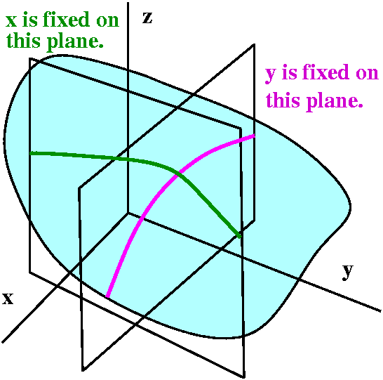
So look at a graph of z=f(x,y). We can slice this in various ways. For
example, we could slice this by a plane
perpendicular to the y axis with y fixed. This will give sort
of an z-x curve. We could "lift" that curve up and just consider it as
a function of one variable, x, and then look at the derivative. That's
 f/
f/ x. Similarly, we could slider by a plane
perpendicular to the x axis with x fixed and consider the
derivative of the resulting curve or function. That will be
 f/
f/ y. Here are the formal definitions if you would like them:
limh-->0(f(x+h,y)-f(x,y))/h= f/ f/ x x
limk-->0(f(x,y+k)-f(x,y))/k= f/ f/ y y
|
I'll use h for little changes in the first variable and k for little
changes in the second variable.
Aiming for first-order understanding
We've already seen that looking at slices is not good enough to
consider limits and continuity. Slices, even collections of slices in
two perpendicular directions, just do not contain enough
information about the function. In the case of f(x,y) and its partial
derivatives, the key idea, both abstractly and computationally, turns
out to be the two dimensional analog of (approximate) local
linearity. If we "kick" the input to f in both x and y, we need to
understand how the function "responds". The nicest response, similar
to one dimension, would be the unperturbed response, f(x,y), then
something proportional to h plus something proportional to y, and,
finally, a higher-order error term. Let's see another example.
 An example
Here is an example related to one I gave last time. Let's look at
f(x,y)=xy/sqrt(x2+y2). Again, things are
"better" (at least for me!) in polar coordinates. Then the bottom
becomes just r (much better!) and the top is
r cos(theta) r sin(theta). The function is
f(x,y)=[r cos(theta) r sin(theta)]/r=r cos(theta) sin(theta). Certainly
on the x and y axes f(x,y) must be 0, because there theta is 0 or Pi
(and the sine factor is 0) or Pi/2 or 3Pi/2 (and the cosine factor is
0). The linearization formula at (0,0) is
f(0+h,0+k)=f(0,0)+ f/
f/ x(0,0)h+
 f/
f/ y(0,0)+higher order error.
Surely
r cos(theta) sin(theta) is 0 when r=0, so f(0,0)=0. And
since f is 0 on all of the x and y axes,  f/
f/ x(0,0)=0 (the slice is
a horizontal line) and
  f/
f/ y(0,0)=0 (this slice is also a horizontal
line). So all of the linearization (the constant term and the first order
stuff) is 0.
But ...
Look at f(0+w,0+w). In the original formula, this is
(0+w)(0+w)/sqrt((0+w)2+(0+w)2) and the result,
after some algebra, is (1/sqrt(2))w. This is first order. But
the linearization is 0. So something is seriously wrong with
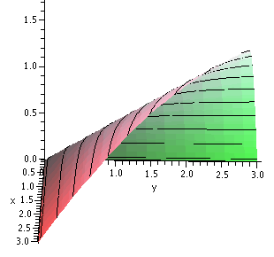
this function. To the right is a picture of the graph of this function
(at least the part which is over the first quadrant). Again, I used a
stalwart (stalwart means "1. strongly built, sturdy. 2. courageous,
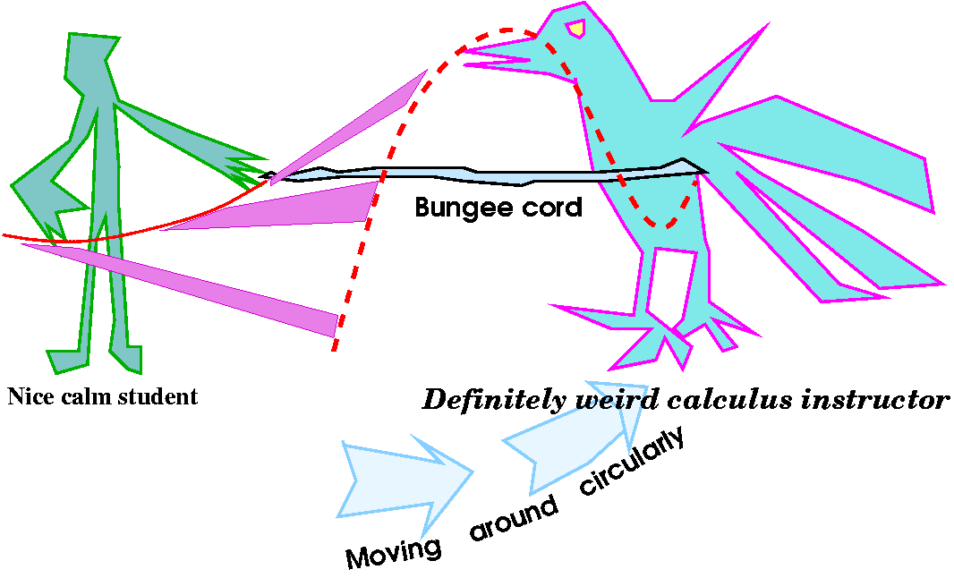
resolute, determined") student volunteer to help. I used the bungee
cords again (is their cost tax-deductible). The process was similar
but not identical to the demonstration last time. The calculus
instructor raised and lowered the cord twice as he walked around the
student. The student this time was asked to keep the end of the cord
always at the same level, not changing at all. This
represented height 0.
Differentiability in 2 dimensions
In mathematics, when something is wrong, one way to help is by making
a definition. The functions we want to consider are called
differentiable and have exactly the property that they can be
approximated nicely.
f(x,y) is differentiable at (x,y) if there are numbers
Constant1 and Constant2 so that for h and k
small,
f(x+h,y+k)=f(x,y)+Constant1h+Constant2+Error,
where the Error term-->0 faster than |h|+|k| (so, faster than first
order).
Important results
Before hysteria strikes, here are two results which are verified in
the text. They are not difficult to check, but we just don't have time
in class.
Theorem If f(x,y) is differentiable, then the partial
derivatives of f(x,y) exist, and Constant1= f/
f/ x(x,y) and
Constant2=
 f/
f/ y(x,y).
Theorem If  f/
f/ x and
x and  f/
f/ y are both continuous then
f(x,y) is differentiable (in the approximation sense defined above).
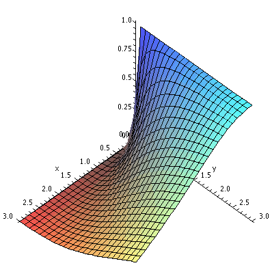
The function f(x,y)=xy/sqrt(x2+y2) has very
lousy (sorry: discontinuous) partial derivatives at (0,0). It is
tedious to check this by hand, but if you plug everything into
Maple then look at graphs ... well, to the right is a graph
of  f/
f/ x in the first quadrant. I hope you can see that the limit as
(x,y)-->(0,0) along the x-axis and along the y-axis seem very
different. So the hypotheses of the previous theorem do not apply to
this function.
Linear approximation: a numerical example
Here we looked at something like
F(x,y)=sqrt(x4-y2+2xy-3). Notice that
F(2,3)=sqrt(24-32+2·2·3-3)=
sqrt(16-9+12-3)=4. This is an example in a calculus class, and it was
chosen so that F(2,3) was nice.
Then
 F/
F/ x=(1/2)sqrt(x4-y2+2xy-2)-1(4x3+2y)
and
 F/
F/ y=(1/2)sqrt(x4-y2+2xy-2)-1(-2y+2x).
We can evaluate these derivatives at (2,3):
 F/
F/ x(2,3)=(1/2)(1/4)(4·23+2·3)=(38)/8 and
 F/
F/ y(2,3)=(1/2)(1/4)(-2·3+2·2)=-2/8.
If we want a linear approximation to F(2.03,2.98), then we may
use the following formula:
F(2.03,2.98) is approximately F(2,3)+ F/
F/ x(2,3)(.03)+
 F/
F/ y(2,3)(-.02).
Here the change in x from 2 to 2.03 means that h is .03 and the change
in y from 3 to 2.98 means that k is -.02. The linearized approximation
gives us 4+(38/8)(.03)+(-2/8)(-.02) which is 4.1475. The "true value"
(well, up to 10 decimal places) of F(2,3) is 4.147314409.
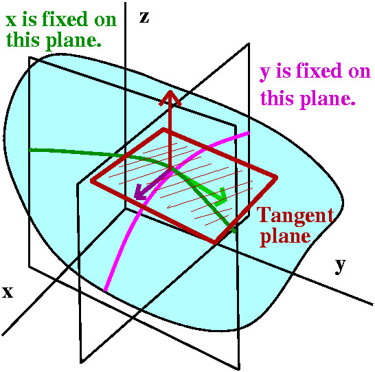 Tangent planes
We can get a bit more out of the slicing picture. The vector i+ f/
f/ xk is tangent to the curve in
R3 gotten by fixing y on the surface z=f(x,y), and the
vector j+
 f/
f/ xk is tangent to the curve in
R3 gotten by fixing x on the surface z=f(x,y). If the
surface is nice and smooth (that is, if the function f(x,y) is
differentiable) people agree that the two vectors determine a plane
which is tangent to
y=f(x,y). To write the equation of a plane, we need a point and a
normal vector.
Suppose we're at the point
(x0,y0,f(x0,y0)). The
normal vector will be perpendicular
to both i+ f/
f/ x(x0,y0)k and j+
 f/
f/ x(x0,y0)k. So we need
to compute the cross product:
[i+
 f/
f/ xk]x[j+
 f/
f/ xk]. So:
( i j k )
det( 1 0  f/
f/ x)=-[
x)=-[ f/
f/ x]i -[
 f/
f/ y]j +k=a normal vector
( 0 1
  f/
f/ y)
y)
I quoted the textbook in class. It states the following result (all
the signs work out correctly!):
If f(x,y) is differentiable, then the equation of a plane tangent to
z=f(x,y) when x=x0 and y=y0 is
(z-z0)= f/
f/ f(x0,y0)(x-x0)+
 f/
f/ y(x0,y0)(y-y0).
QotD
I think it was something like this: write the equation of a plane
tangent to z=x2y when x=2 and y=3.
HOMEWORK
Almost surely there will be an exam two weeks from today's lecture, in
class, on Friday, February 24. More definite information will be
available on Tuesday. Now you should work on your Maple
assignments and other homework.
Answers to these problems should be handed in at the recitation on
Wednesday, February 15. Please try to read and learn these sections of
chapter 14 by then: up to 14.5, doing the appropriate problems.
14.3: 21, 48;
14.4: 6, 17;
14.5: 35, 46;
Tuesday, February 7
Operational matters
Office hours for the lecturer this semester will be:Tuesday from 1:40 to 3:00
Thursday from 2:00 to 4:00
in Hill 542. But the lecturer (that is, me) is in most days,
and the scheduled office
hours are not convenient or you need a different time,
please talk to me or better, send e-mail if you'd like to find a
mutually agreeable time for discussion which isn't at a scheduled
office hour.
Maple Data for another assignment
has been sent to students. Any student who did not get data should
send me e-mail, please!
Functions of "several" variables
We move on to one of the major topics of the course. The word
"several" is almost technical in mathematics, and means "more than
1". We will start with an almost ludicrously simple function.
x2+y2
Here f(x,y)=x2+y2. This is a function defined by
a formula (essentially all of the functions we'll consider in this
course will be defined by formulas). The notation means that the input
to the function is an ordered pair of numbers, (x,y), and the output
is one number. Here the output for the ordered pair (-2,3) is 13.
Formalities: domain and range
The domain will be the collection (the "set") of all possible
inputs. Just as in calc 1, if the function is defined by a formula,
then the domain will be all inputs for which the function makes
sense. The usual restrictions that will concern us are:
- Don't divide by 0.
- Square roots of non-negative numbers only (same for other even
roots).
- Logarithms only for positive numbers.
These should all be familiar to you.
The range will be the collection of all possible outputs. You
may remember from calculus that while determining precise domains is
often possible but tedious, precise descriptions of ranges can be
quite difficult (this can involve exact determinations of max and min
values).
Here are some examples chosen to illustrate the likely possible restrictions. I certainly did not have time to discuss all
of these in class.
| f(x,y)=x2+y2 |
|---|
Domain
I think all pairs (x,y) of real numbers, all of R2.
|
Range
Since squares are non-negative, certainly the values of this function
are non-negative. And f(0,0)=0, and f(sqrt(A),0)=A for A positive. I
am just verifying precisely that the range is all non-negative real
numbers.
|
| f(x,y)=1/(y-x2) |
|---|
Domain
So this example is chosen to illustrate the restriction about not
dividing by 0. The domain is
all pairs (x,y) of real numbers for which y is not equal to
x2. Geometrically, this means all points of R2
which are not on the parabola y=x2.
|
Range
Well, 0 isn't in the range (it isn't the reciprocal of any
number). But everything else is: check this by just looking at what
happens to (0,A), which gives 1/A for all non-zero A's.
|
| f(x,y)=sqrt(y-x2) |
|---|
Domain
So this example is chosen to illustrate the restriction about square
roots. The parabola y=x2 divides R2 into two
pieces. One piece contains, say, the point (3,4) ("below" the
parabola). This point has y-x2=4-32=-5<0, so
(3,4) is not in the domain of this function. The domain is the
"other" piece of R2 and also those points which are on the
curve y=x2.
|
Range
The range is all non-negative numbers. Again, to check this you could
look at what happens to (0,A) for A>=0.
|
| f(x,y)=ln(y-x2) |
|---|
Domain
I still must "throw out" the part of R2 which is below the
parabola. But here inputs to ln must be positive, so the domain
does not include the curve y=x2. The domain is all of the
points in R2 which are above the parabola.
|
Range
The range is the range of ln, which is all real numbers.
|
Kinds of graphs
|
Let me return to the simplest of the functions I just considered:
f(x,y)=x2+y2. There are various graphs which are
commonly used. Maybe the simplest is to consider the points (x,y,z) in
R3 which satisfy the equation
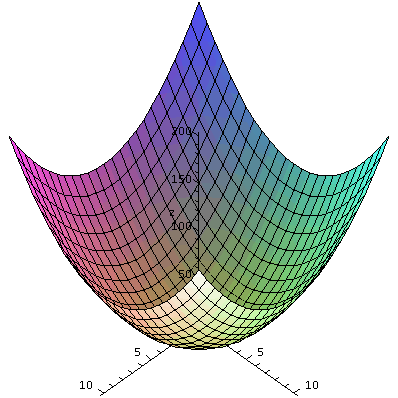
z=x2+y2: this is usually called the graph of
the function. A Maple representation of this graph is
shown to the right, and the procedure which produced it is
plot3d, part of the plots package. This is rather a
simple function, and I hope you can see the shape of this surface. It
is a cup, axially symmetric around the z-axis. It is called a
paraboloid.
|
|
Another kind of plot, or, anyway, some geometric clue to the nature of
the function, can be gotten by looking the contours of f(x,y). There
are topographic maps (say, used by hikers) which give a
two-dimensional representation of the information in the surface
picture above. Pick a constant, C, and look at the (implicitly
defined) "curve" f(x,y)=C. I put quotes around the word "curve"
because maybe it doesn't have to be a neat nice curve. (An example was
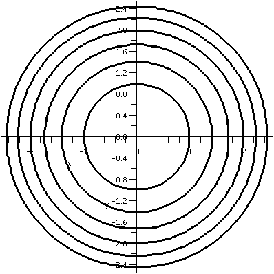
discussed in class, and is below.) To the right is a collection of
contours for f(x,y)=x2+y2. These contours
correspond to the positive integers 1, 2, 3, 4, 5, and 6.
Please notice how these contours, which are at evenly spaced
"heights", get closer together as the three-dimensional graph gets
steeper. Of course, if the contours are not labeled with the values of
the constants, I can't tell if the function is increasing or
decreasing! This picture was made with contourplot, another
part of the Maple package, plots.
|
|
 Two half planes
I then turned our attention to a function which initially looks
simpler, but whose graph is perhaps more bizarre.
        ( x  if x>0
f(x,y)= (
        (2x if x<=0
We explore this function more slowly. We computed some sample values:
f(3,4)=3 ,f(-3,4)=-6 ,f(3,-4)=3 ,f(-3,-4)=-6.
Then for the geometric side: I believe I first sketched the
intersection of the graph z=f(x,y) with the xz-plane, and got a
"broken line". The function really doesn't depend on y, so the graph
can just be stretched back and forth perpendicular to the xz plane to
get the whole three dimensional graph. The graph z=f(x,y) is two
half-planes joined at the y-axis. A version of the graph is shown
to the right.
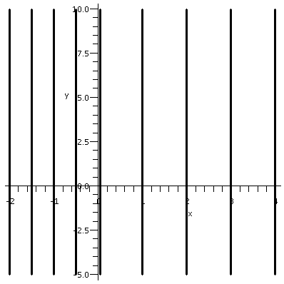 I also tried to sketch the contour lines. What's shown to the right is
a picture of the contour lines of this f (that is, f(x,y)=C in
R2) for C integer valued ranging from -4 to 4. The contour
lines are lines perpendicular to the x-axis (indicating the lack of
dependence on y in the function). The contour lines are spaced twice
as far apart in the right halfplane as in the left halfplane,
indicating that the function f(x,y) in the left halfplane (where
x<0) increases faster than in the right. Indeed, that's a
reflection of the 2 in the definition.
Incidentally, Maple allows such functions to be defined with
the piecewise command. As we'll see, the graphing routines
don't always display the graphs correctly, because there are some
assumptions of continuity.
How the bug increases
I remarked that if a bug were placed in R2 and wanted to
move to increase its value of f(x,y) as much as possible, it would
move perpendicularly to the contour lines.
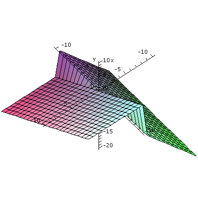 Another two half planes
I defined another piecewise function. It seems to be only slightly different from the previous one, but the graph is, to me, much "worse".
        ( y  if x>0
f(x,y)= (
        (2x if x<=0
First, this function does depend on y. So we computed:
f(3,4)=4 ,f(-3,4)=-6 ,f(3,-4)=-4 ,f(-3,-4)=-6.
We discussed the graph of z=f(x,y). Again I think I began with what
happens on the xz-plane. After some exchanges we decided this was
again a broken line, but the right half of the line (where x>0) was
horizontal, with z=0. More globally, the "rear" halfplane (where
x<0) is the same as the previous function's graph. The front, where
x>0, was a plane which was tilted up as y increased. The graph that
is shown is Maple's version. Please notice that
Maple attempts to "connect the dots" in a rather crude way:
this is the graph of a function so there are no vertical line
segments in this graph, such as appear in the version shown.
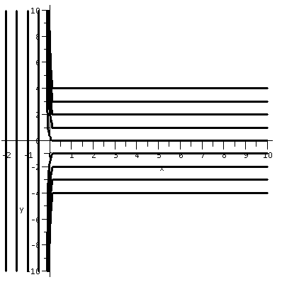 The contour lines are also not sketched too well. Most particularly,
the contour "line" f(x,y)=0 is very peculiar. It actually consists of
the y-axis together with the positive x-axis. Maple doesn't
want to draw anything like that, so it actually omits a line segment
in this T-shaped contour line. I tried various options with
contourplot but I could not get the T contour (C=0) drawn
correctly. The other contours are again for integer level sets. The
level sets for C>0 are horizontal half lines in the first
quadrant. The level sets fo C<0 have two pieces. One part is a
horizontal half line in the fourth quadrant, and one part is a whole
vertical line in the left halfplane. This may be hard to visualize. I
urged people to try to educate their intuition. The left lines are
closer together than the horizontal halflines.
The suicidal bug
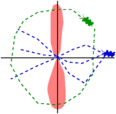 Now comes some of the harder stuff. I asked people to imagine that
some bugs were "walking" on the graph of z=f(x,y). The green bug, whose path is shown to the
right, strolls along in a path which is roughly circular around the
origin. This bug runs into trouble at any point on the positive
y-axis, where there's a drop. It also has problems along the negative
y-axis, where again there is a big difference in heights. This is a
very small bug. I have tried to indicate this by a sort of light
reddish color surrounding these half-lines. The
blue bug walks from the right halfplane to the left
halfplane. It is careful to cross only at the origin. The blue
bug is totally safe, and never comes across any severe height
differences. So I would like to discuss (and name [define], since it
is a math course!) the differences the bugs encounter more precisely.
Limits in one dimension
In one variable, limits are relatively simple. To define
limx-->af(x) we look at how x gets close to a from both
sides. There are some standard pictures and standard examples of
bad situations. Below are a few, to remind you.
| Bad limiting behavior in dimension
1 |
|---|
A jump
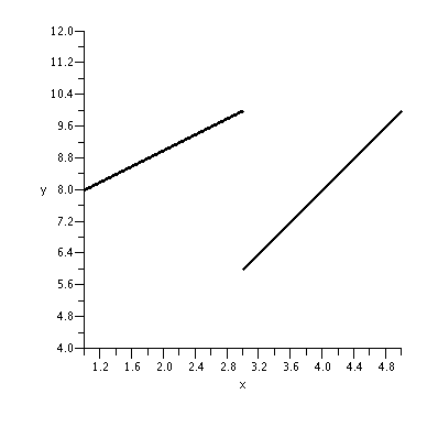
(y=x+7 for x<3, and 2x otherwise.)
|
Many wiggles
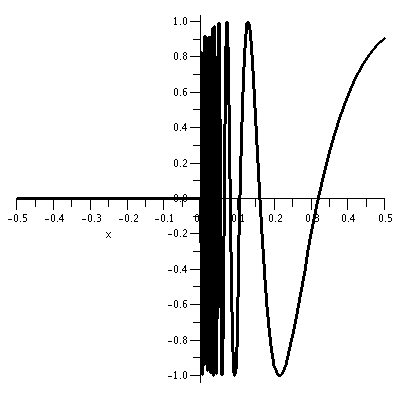
(y=sin(1/x) for x positive, y=0 otherwise.) |
Several variables
In several variables limiting behavior can be quite complex, much more
than with one variable. I tried to give a few examples.
Many straight line limits exist
I asked students to consider the function
f(x,y)=xy/(x2+y2)
This is an algebraic
formula which behaves is a strange fashion for (x,y) near (0,0). We
could try some values, but we can also take advantage of the
appearance of x2+y2. Almost always that's a
signal to at least attempt to understand things in polar coordinates
-- that is, to take advantage of circular symmetry.
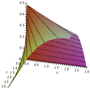
Since x=r cos(theta) and y=r sin(theta), we know that
x2+y2=r2 and
xy=r2cos(theta)sin(theta). Therefore
f(x,y)=xy/(x2+y2)=cos(theta)sin(theta)
The
value of f(x,y) only depends on the angular part of the polar
coordinate representation of (x,y) and not at all on the radial
component. The graph is made up of a bunch of half lines all parallel
to the xy-plane, radiating out from the z-axis. These halflines, since
cos(theta)sin(theta)=(1/2)sin(2theta), all have height between -1/2
and +1/2.
A Maple graph of the surface over the first quadrant (x>0
and y>0) is shown to the right. I also attempted, with the help of
a stalwart student accomplice, to "draw" the surface kinetically. The
student "volunteer" held one end of a bungee cord under some tension
(both in the student and the cord!) while the calculus instructor held
the other end and walked around the student. The calculus instructor
raised and lowered the cord twice and the student was asked to keep
the end of the cord at the same level as the instructor's
end. Therefore along every angle a limit existed, but as the angle
changed, the limits changed. There were infinitely many
different limits possible along straight line approaches to
(0,0).
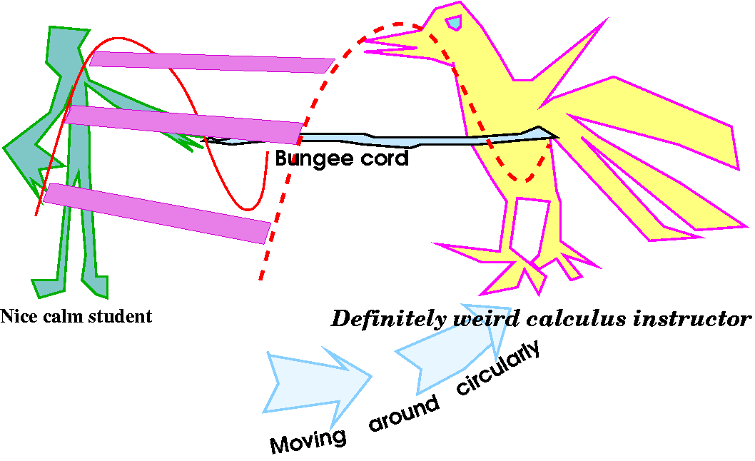
Always 0 on a straight line approach
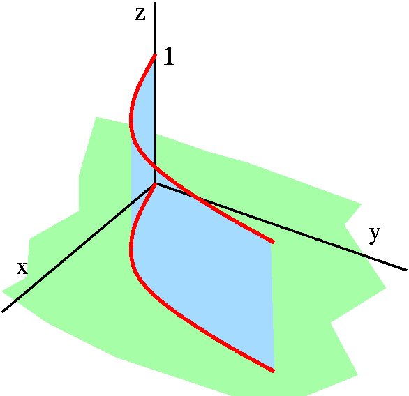 The final example of this lecture was the following function:
        ( 1  if y=x2 and x>0
f(x,y)= (
        ( 0 otherwise
This function has only two values, 0 and 1. Certainly if you "walk"
towards 0 on a straight line approach in the second, third, and fourth
quadrants, the function values are all 0 and therefore the limit is
0. What's not so obvious perhaps is the behavior of the function on
straight line approaches in the first quadrant.
Look at y=x. This line intersections y=x2 only at x=0 and
x=1. So if we "walk" towards the origin on this line from some large
x>0 considering the values of the function f(x,y), the function
will be 0 at every point except x=1 where it will be 1. Certainly the
limit as x-->0 will exist, and it will be 0.
In fact, the limit exists on every straight line approach to (0,0),
and the value of the limit is 0. But the real, two-variable limit
should not exist, because the values of f(x,y) do not get close to 0
as (x,y)-->(0,0).
QotD
I introduced  by just using
it.
Example 1 If F(a,b,c)=a2b-3bc3 then
 F/
F/ a=2ab and
  F/
F/ b=a2-3c3 and
 F/
F/ c=-9bc2.
Example 2 If F(a,b,c)=a3sin(7b-5c2) then
 F/
F/ a=3a2sin(7b-5c2) and
 F/
F/ b=a3cos(7b-5c2) and
 F/
F/ c=a3cos(7b-5c2)(-10c).
The QotD was to find  F/
F/ a and
a and  F/
F/ b and
b and  F/
F/ d is F(a,b,c) was
something like (a3-5b2)/(bc3-4a).
HOMEWORK
Answers to these problems should be handed in at the recitation on
Wednesday, February 15. Please try to read and learn these sections of
chapter 14 by then: up to 14.5, doing the appropriate problems.
14.3: 21, 48;
14.4: 6, 17;
14.5: 35, 46;
Maintained by
greenfie@math.rutgers.edu and last modified 2/13/2006.
 Example #1
 Compute the gradients, etc.
Then the multiplier equations and the constraint equation
are:
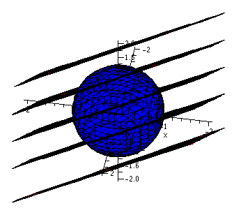
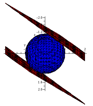


 By the way, the type of functions illustrated in the first and third
pictures are called piecewise linear. In lots of variables, finding
extreme values of these functions is rather difficult. The problems
are wildly varied, and can deal with topics like scheduling and
allocation. You could begin with an undergrad course to study the
math of these problems (Linear Optimization) and then look into
various aspects of Operations Research or Industrial Engineering.


 Ridiculous interesting (?) fact
 Monkey saddle
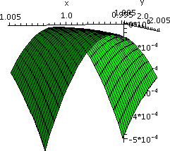
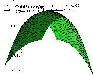
 The pictures certainly shouldn't be convincing evidence, but they do
support the textbook's assertion that the function has local minimums
at both critical points! (We can verify this assertion with the second
derivative test to be stated later.)
Why do I find this disconcerting? Well,
imagine we walk from one peak to another (shown to the right, the
blue "trail").
  Shouldn't we somehow pass through a saddle? Well, in
fact, no, we don't need to: maybe the lowest point on the blue trail
is not a critical point -- the tangent plane to the surface at that
point may be tilted. In this example, the tangent plane is
always tilted at every point except the two peaks.
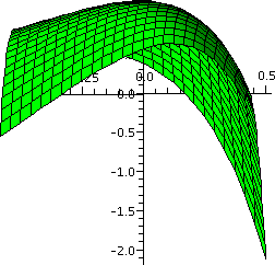
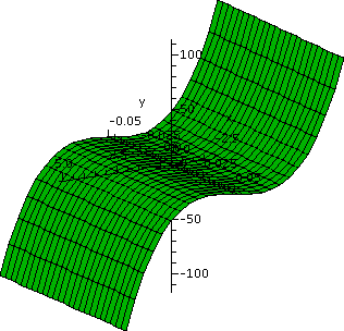

 sloth laziness or indolence; reluctance
to make an effort.
 From this we can see that the temperature measured at the rocket at
time t is T(t)=T(x(t),y(t),z(t)), and this is a composition. First we
find out where the spaceship is at time t, and then we compute the
temperature at that point.
 Observation 3
 A better example (!)
 Ellipsoid


 Slicing and partial derivatives
 An example

 Tangent planes

 Two half planes
 I also tried to sketch the contour lines. What's shown to the right is
a picture of the contour lines of this f (that is, f(x,y)=C in
R2) for C integer valued ranging from -4 to 4. The contour
lines are lines perpendicular to the x-axis (indicating the lack of
dependence on y in the function). The contour lines are spaced twice
as far apart in the right halfplane as in the left halfplane,
indicating that the function f(x,y) in the left halfplane (where
x<0) increases faster than in the right. Indeed, that's a
reflection of the 2 in the definition.
 Another two half planes
 The contour lines are also not sketched too well. Most particularly,
the contour "line" f(x,y)=0 is very peculiar. It actually consists of
the y-axis together with the positive x-axis. Maple doesn't
want to draw anything like that, so it actually omits a line segment
in this T-shaped contour line. I tried various options with
contourplot but I could not get the T contour (C=0) drawn
correctly. The other contours are again for integer level sets. The
level sets for C>0 are horizontal half lines in the first
quadrant. The level sets fo C<0 have two pieces. One part is a
horizontal half line in the fourth quadrant, and one part is a whole
vertical line in the left halfplane. This may be hard to visualize. I
urged people to try to educate their intuition. The left lines are
closer together than the horizontal halflines.
 Now comes some of the harder stuff. I asked people to imagine that
some bugs were "walking" on the graph of z=f(x,y). The green bug, whose path is shown to the
right, strolls along in a path which is roughly circular around the
origin. This bug runs into trouble at any point on the positive
y-axis, where there's a drop. It also has problems along the negative
y-axis, where again there is a big difference in heights. This is a
very small bug. I have tried to indicate this by a sort of light
reddish color surrounding these half-lines. The
blue bug walks from the right halfplane to the left
halfplane. It is careful to cross only at the origin. The blue
bug is totally safe, and never comes across any severe height
differences. So I would like to discuss (and name [define], since it
is a math course!) the differences the bugs encounter more precisely.


 The final example of this lecture was the following function: