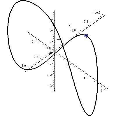
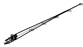
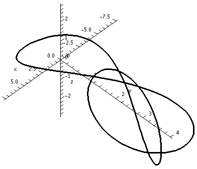
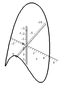
This first picture shows the
result of the command
>spacecurve(Q(t),t=0..2*Pi);
I had previously defined Q(t) with a command that looked like this:
>Q:=t-><5*cos(2*t)+5*sin(t),2*cos(2*t)+4*cos(t),sin(3*t)+4*sin(t)>
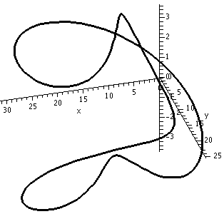
The result is the picture shown below.
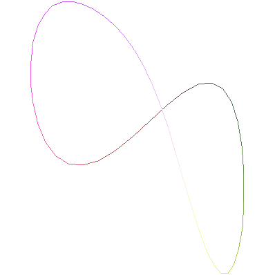
>spacecurve(Q(t),t=0..2*Pi,thickness=2,color=black,axes=normal,
labels=[x,y,z],numpoints=150);
All commands should be typed on one line.
They're on several lines here to control the web page's width.
I used "options" which I specified after some experimentation. The thickness and color made the curve easier to see. The labels on the axes are also useful if the image is rotated. The numpoints option increases the number of sampling points, because mostly what Maple does is plot points (the default, I think, is 50) and then connect these points with straight line segments. If you want to play, see what happens with numpoints=20 or numpoints=10. You'll get very polygonal (corners, line segments) approximations to the curve. The increases specification for numpoints made the curves I experimented with seem less polygonal.
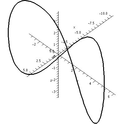
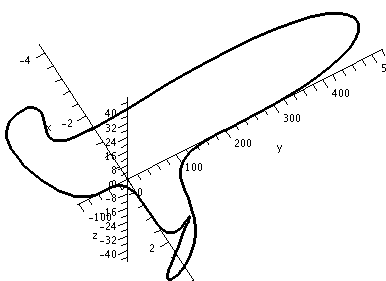
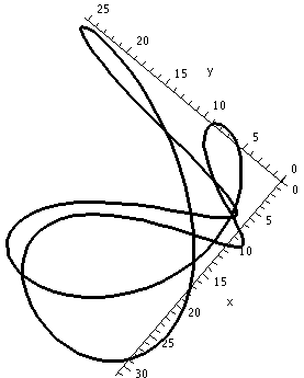
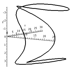
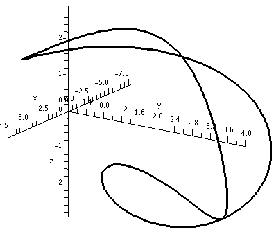
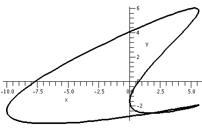
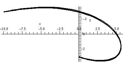
Warning There are curves which do not intersect themselves, but have the irritating (?) property that every two dimensional view shows intersections!
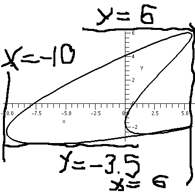
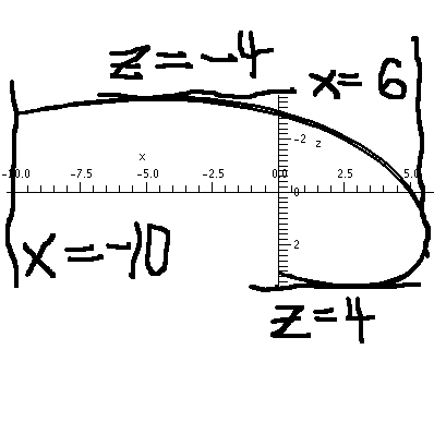
The image on the left has the z-axis sticking directly out from the viewing plane.
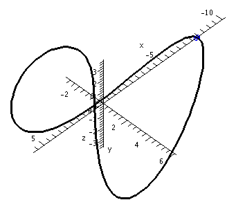
The image on the right has the y-axis sticking directly out from the viewing plane. Therefore it shows a picture of the curve squooshed (??) down on the xz-plane. Unfortunately (?) due to carelessness, the z-axis is inverted from its standard presentation (positive is down in this picture and negative is up).
> dsdt:=Norm(diff(Q(t),t));
dsdt:=((-10*sin(2*t)+5*cos(t))^2+(-4*sin(2*t)-4*sin(t))^2+(3*cos(3*t)+4*cos(t))^2)^(1/2)
If we want the length, we need to integrate this from t=0 to t=2Pi. Here is what happened when I tried a "direct" computation on my computer at home and also requested, before and after the computation, the amount of CPU time used.
> time(); .222 > int(dsdt,t=0..2*Pi); int(((-10*sin(2*t)+5*cos(t))^2+(-4*sin(2*t)-4*sin(t))^2+(3*cos(3*t)+4*cos(t))^2)^(1/2),Maple returned the original integral, not evaluated, although the program did "think" about it for almost a dozen CPU seconds! This tells me that Maple was unable to evaluate this integral symbolically, which is not surprising -- "most" functions defined by formulas can't be antidifferentiated in terms of familiar functions.
t=0..2*Pi); > time(); 12.114
Maple needs to be "convinced" to evaluate this integral
approximately. Here's how to do that:> evalf(Int(dsdt,t=0..2*Pi));
56.13189562
Please note the capital I in the
integrate command. This is an important difference which you can read
about on a help page if you want. The numerical computation of the
integral took less than a hundredth (.01) of a second. This curve
is about 56 units long.

This is not Maple's Norm.
(He is a master carpenter on a TV show about
home renovations called This Old House.)
> Curvature(Q(t),t);
((-1/2/(-200*sin(t)*cos(t)^2+144*cos(t)^6-584*cos(t)^4+498*cos(t)^2+64*cos(t)+
16-64*cos(t)^3)^(3/2)*(-10*sin(2*t)+5*cos(t))*(-200*cos(t)^3+400*sin(t)^2*cos(
t)-864*cos(t)^5*sin(t)+2336*cos(t)^3*sin(t)-996*sin(t)*cos(t)-64*sin(t)+192*
sin(t)*cos(t)^2)+1/(-200*sin(t)*cos(t)^2+144*cos(t)^6-584*cos(t)^4+498*cos(t)^
2+64*cos(t)+16-64*cos(t)^3)^(1/2)*(-20*cos(2*t)-5*sin(t)))^2+(-1/2/(-200*sin(t
)*cos(t)^2+144*cos(t)^6-584*cos(t)^4+498*cos(t)^2+64*cos(t)+16-64*cos(t)^3)^(3
/2)*(-4*sin(2*t)-4*sin(t))*(-200*cos(t)^3+400*sin(t)^2*cos(t)-864*cos(t)^5*sin
(t)+2336*cos(t)^3*sin(t)-996*sin(t)*cos(t)-64*sin(t)+192*sin(t)*cos(t)^2)+1/(-\
200*sin(t)*cos(t)^2+144*cos(t)^6-584*cos(t)^4+498*cos(t)^2+64*cos(t)+16-64*cos
(t)^3)^(1/2)*(-8*cos(2*t)-4*cos(t)))^2+(-1/2/(-200*sin(t)*cos(t)^2+144*cos(t)^
6-584*cos(t)^4+498*cos(t)^2+64*cos(t)+16-64*cos(t)^3)^(3/2)*(3*cos(3*t)+4*cos(
t))*(-200*cos(t)^3+400*sin(t)^2*cos(t)-864*cos(t)^5*sin(t)+2336*cos(t)^3*sin(t
)-996*sin(t)*cos(t)-64*sin(t)+192*sin(t)*cos(t)^2)+1/(-200*sin(t)*cos(t)^2+144
*cos(t)^6-584*cos(t)^4+498*cos(t)^2+64*cos(t)+16-64*cos(t)^3)^(1/2)*(-9*sin(3*
t)-4*sin(t)))^2)^(1/2)/(-200*sin(t)*cos(t)^2+144*cos(t)^6-584*cos(t)^4+498*cos
(t)^2+64*cos(t)+16-64*cos(t)^3)^(1/2)
This is certainly an example of why people use : instead of ;. The colon doesn't display its output. I think that knowledge of the specific formula of the curvature is not likely to be useful.
But I can compute the curvature at, for example, t=2:
> evalf(subs(t=2,Curvature(Q(t),t)));
.2586332282
The subs command substitutes 2 for t in the result of the Curvature(Q(t),t) command, and then evalf asks for a digital approximationBBB.
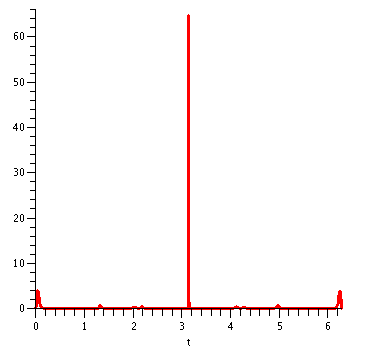
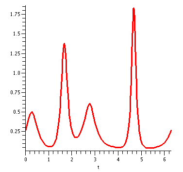
Below is the result of the command
plot(Curvature(Q(t),t),t=0..2*Pi,thickness=2);
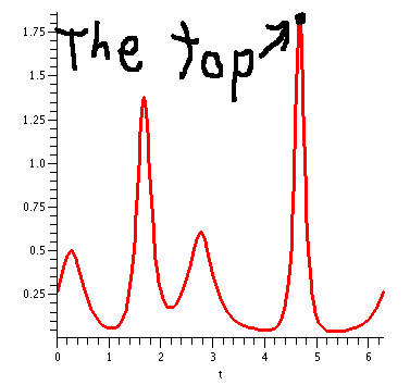
>evalf(subs(t=4.69,Q(t)));
Vector[column](3,{(1) = -9.993735059, (2) =
-2.087543709, (3) = -3.001252360}, datatype = anything,storage =
rectangular,order = Fortran_order,shape = [])
The same command in the GUI (graphical user interface) gives a cleaner
answer, but the answer in both is about (-9.994,-2.086,-3.001).
Now I'll try to locate the point, the most curvy point, on the
graph. I'll create two pictures, and then
display them together:> MCP:=plot3d([-9.994,-2.086,-3.001],x=-10..5,y=-5..5,labels=[x,y,z],
The picture on the left was displayed. I was confused. The little
blue box is supposed to be the MCP ("most
curvy point"). But what's near the MCP candidate didn't look very
curvy compared to other parts of the curve. But then I "adjusted" the
image to Scaling=Constrained and the
result was the picture on the right. I was happier.
symbol=box,axes=normal,color=blue,style=point):
> CURVE:=spacecurve(Q(t),t=0..2*Pi,thickness=2,color=black,axes=normal,
labels=[x,y,z],numpoints=150):
> display({MCP,CURVE})
