17≠0).
The computation I did for sine above is actually a bit more
general. Here is a result which is sometimes useful.
Fact An analytic function f(z) has a zero of order n at p
(where n is a positive integer) exactly when
f(z)=(z–p)nh(z(), h(z) analytic near p and h(p)≠0,
or f(p)=0, f´(p)=0, f´´(p)=0, ...,
f(n–1)(p)=0, and f(n)(p)≠0.
Analytic functions can even have zeros of unbounded order
(construction of this is not so simple). Although such a function can
have infinitely many zeros, there is a slightly subtle restriction on
the geometry of the zeros.
| Monday,
April 12 | (Lecture #21) |
|---|
I began class by writing a version of the Residue Theorem as George
Green might have imagined it. After this was attacked, I sullenly
retreated to a mathematical formulation which I used for the balance
of the lecture. I did remark that our previous results on integrals
(Cauchy's Theorem, the Cauchy Integral Formula, and the Cauchy
Integral Formula for derivatives) could all be regarded as special
cases of the Residue Theorem.
Residue examples
The Fourier transform of 1/(1+x2)
∫–∞∞[cos(mx)/(1+x2)]dx
Maple says this should be
–Πsinh(|m|)+Πcosh(|m|).
Here the "surprise" is that we do not take f(z) to be
cos(mz)/(1+z2) because that would not have growth which
would be easy to estimate on the upper semicircle. Instead, for
m>0, take f(z)=eimz/(1+z2). This f(z) has a
simple pole at i, so f(z)=h(z)/(1-i). Then res(f;i)=h(i).
|  |
∫–∞∞[ln(x)/(1+x2)2]dx
Here we needed an indented contour to take
care of problems at 0. The integrand had to be chosen with some care
in order to get a good definition of log. We took
f(z)=Log(z)/(1+z2)2. f(z) has a double pole at
i, and if f(z)=h(z)/(z-i)2, then res(f;i)=h´(i).
This should be –Π/4 (with 1+x2 downstairs the
integral is 0 -- use a cute change of variables: x→1/x to see
this "clearly").
|  |
∫0∞dx/(1+x4)
(Two simple poles. With luck skill, the result is real and even
positive.)
This should be Πsqrt(2)/4. My hurried computation did not quite get
this, I think. The residue computation was gotten (if the simple pole
is at, say, r) by looking at
limz→r(z-r)/(1+z4) and using L'Hop.
|
|
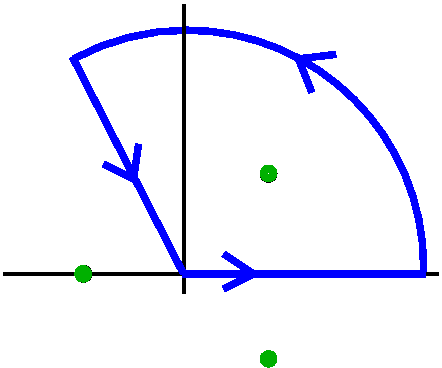
∫02Πdθ/(5+3sin(θ)).
Clearly (NO!) change the integral into an integral around
the unit circle.
We already did this integral in lecture #??. You can inspect what we
did and find the Residue Theorem "lurking" in the computation.
|  |
∫0∞dx/(1+x3)
Many coincidences. Choosing the correct contour works, but
it is emphatically not obvious!
This should be 2Πsqrt(3)/9.
| 
|
There are whole books about the use of the Residue Theorem in
computing integrals (proper and improper) and in computing infinite
series.
Mr. Cantave remarked after class that
it seems all the examples I showed could be done in various ways
without the Residue Theorem itself. I had looked at poles, where the
results could maybe have been gotten with various manipulations
involving the Cauchy Integral Formula. That is certainly correct as
far as the examples we've seen. But there are other more complicated
situations where the Residue Theorem itself is a more appropriate
tool. I don't have time to show you those.
| Wednesday,
April 7 | (Lecture #20) |
|---|
Example 1
Look at
f(z)=(z–2)3/[z5(z+i)2]. f has
isolated singularities at 0 and –i. What happens at, say,
–i? Well, I can write f(z)=(z+i)–2h(z) where
h(z) is analytic near –i and h(–i)≠0. Here we can take
h(z)=(z–2)3/z5 so that
h(–i)=(–i–2)3/(–i)5: I
don't much care what it is right now other than noticing that it
isn't equal to 0. So f(z) has a pole of order 2 at
–i. Also (same sort of logic) f(z) has a pole of order 5 at 0.
Example 2
Let's consider f(z)=z/sin(z). I know that
sin(z)=sin(x+i y)=sin(x)cos(i y)+cos(x)sin(i y)=sin(x)cosh(y)+i cos(x)sinh(y).
Note that since cosh(y) is never 0, this is 0 only when sin(x)=0. Note
that to get the imaginary part=0, we need y=0 since cos(x) will
never be 0 when sin(x)=0. So the zeros of sin(z) are when
z=(integer)Π.
Suppose n is an integer. What does the power series for sine look
like at nΠ? Since sin(nΠ)=0 and cos(nΠ)≠0 (yeah, yeah, I'm
too busy to notice whether n is even or odd -- I just care if things
aren't 0 right now!). So
sin(z)=0+A(z–nΠ)+0(z–nΠ)2+B(z–nΠ)3+H.O.T..
There are now two cases:
- n=0. Here
f(z)=z/[0+Az+0z2+Bz3+H.O.T.]=1/[A+0z+Bz2+H.O.T.]
and what is on the bottom is a convergent power series because I got
it by factoring out a z from a convergent power series. Therefore
limz→0f(z)=1/A≠0 so f(z) has a removable
singularity at 0.
- n≠0. Now
f(z)=z/[0+A(z–nΠ)+0(z–nΠ)2+B(z–nΠ)3+H.O.T.].
I notice that as z→nΠ, the top→nΠ≠0, while the
bottom→0. We can write f(z)=(z–nΠ)–1h(z), where
h(z)=z/[A+0(z–nΠ)1+B(z–nΠ)2+H.O.T.]
is a function analytic near nΠ and h(nΠ) is (nΠ/A)≠0. So
this f(z) has a pole of order 1 (frequently called a simple
pole [I will make an appropriate joke about this at some time!])
at nΠ.
If you want more elaborate examples, you can get them by, say,
considering something like
f(z)=z(z+Π)2(z–2Π)3/[sin(z)]2. I
claim that f(z) has isolated singularities at nΠ where n is an
integer. For n=0, the singularity is a simple pole (a pole of order
1). For –Π, the singularity is removable. For 2Π, the
singularity is removable (and the value is 0: in fact, the resulting
function has a zero of order 1). For other n's, f(z) has a double pole
(pole of order 2).
 Example 3
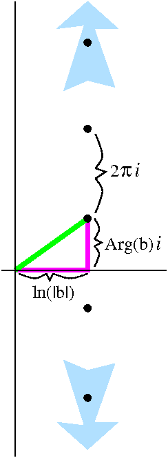
Take f(z)=e1/z. Since I know its Laurent series (take
∑n=0∞zn/n! and stuff in 1/z
for z to get
∑n=0∞{1/n!}z–n, which
certainly has infinitely many non-negative coefficients. But also I
know that I can solve e1/z=b (for b≠0) whenever
1/z=log(b). This means 1/z=ln(|b|)+i Arg(b)+2Πn i, so
that z=1/[log(|b|)+i Arg(b)+2Πn i]. Since the sequence
log(|b|)+i Arg(b)+2Πn i→∞ as n→∞, I
know that the sequence of reciprocal entries→0 as n→0.
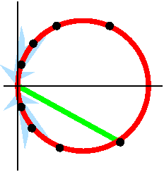
The pictures illustrating this are to the left and to the right.
On the left Those are supposed to be some representatives of
the set log(b). There's a specified Log(b) with some colors,
and the other elements are translations up and down by 2Π i
of Log(b). There are infinitely many of them, of course.
On the right These complex numbers are reciprocals (1/z) of the
numbers in the first picture. It happens that a vertical line becomes
(under the transformation z→1/z) a circle going through 0 (I'll
show you soon a rapid way to verify that instead of using
computation). As the dots in the left picture sail up and down by
multiples of 2Π i, the images in the right are a sequence
which →0 in two ways.
This illustrates a strong version of the qualitative consequence of
Casorati-Weierstrass. The values of e1/z are not only are
close to b's, but they are equal to b's (with one exception, b=0).
This example is not an accident. There is a much more "powerful"
result called The
Great Picard Theorem which asserts that if f(z) has an
essential singularity at 0, then on any open neighborhood of 0, f(z)
takes all possible values, with at most one possible exception. For
e1/z, the exceptional value is 0. The Big Picard Theorem is
difficult to prove.
Discussion question
Where does f(z)=e1/[sin(1/z)] have isolated singularities,
and what kind of singularities are they? Well, the function is not
defined where sin(1/z)=0 or where 1/z is not defined, and that's
where z=1/[nΠ] and z=0. So candidates are those numbers. But (trick
question!) z=0 is not an isolated singularity! It is not
isolated, since it is a limit point of other places where f(z) is not
defined. All of the 1/[nΠ] points are isolated singularities, and
they are essential.
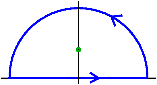
 Baby Residue Theorem
Suppose f is analytic in 0<|z–p|<R and C is a simple closed
curve in that disc with p inside C. Then
∫Cf(z) dz=2Π i a–1, where
a–1 is the coefficient of (z–p)–1 in the Laurent
series for f in 0<|z–p|<R.
First write out the Laurent series for f, and then interchange
integration and summation (this is valid because we have nice error
estimates for the series). Then notice that all the other
pieces of the Laurent series, C(z–p)N for N≠–1 are
derivatives of analytic functions, C(z–p)N+1/(N+1), and we
know that the integral of g´ around a closed curve is 0. Then we
deform C into a small circle around p and get just our "usual
suspect", a–1∫1/(z–p) dz, giving us the desired result
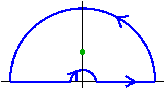
2Π i a–1. We could also think, instead of a
deformation, that there is sort of a crosscut going back and
forth between the small circle and C. Then "inside" the contour gotten
by going around C, down the crosscut to the circle, backwards around
the circle, and up again using the crosscut, we have a region in which
f is analytic, so (Cauchy's Theorem!) the integral is 0. But the
crosscut integrals (in green in the
picture) cancel each other, and then the integral around C minus the
integral around the circle (backwards) have total value 0. So the two
integrals are equal.
This is a prototype for one of the most interesting results in
mathematics, the Residue Theorem. Your text calls this a–1
the Residue of f at p, and written Res(f;p). Please: other
texts and references have different notations.
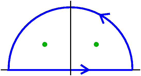
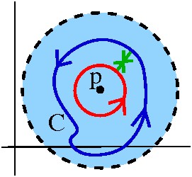
 More grownup Residue Theorem
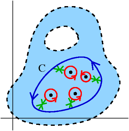
Suppose C is a simple closed curve in a connected open set U, and f is
analytic on and inside C except possibly for a finite number of
isolated singularities inside C. Then
∫Cf(z) dz=2Π i ∑p isol. sing. inside CRes(f,p).
This result has been tremendously influential in mathematics and its
applications. One reason is that it compares global and local
information. The integral is some sort of "global" information about f
on C. The Residue Theorem says that this equals a sum (a finite sum)
of "local" data about f, these residues.
Proof There are many very elaborations of this result, Here in
Math 403, I see the verification of the result is a consequence of a
picture which is displayed to the right. There is C, and there are
displayed the isolated singularities of f inside C. Look at the
picture, consider the crosscuts and realize
that we're done: each of the circles contributes the residue at the
center of the circle, and the crosscut integrals all cancel out. We're
done!
Secret strategy We're using different Laurent series
representations around and inside each circle!
Workshop problem
Now the instructor will distribute the workshop problem and students will
work in small groups to complete the problem.
It was a wonderful occasion. Many people were able to do almost
all of the workshop. Let me discuss the solutions in some detail.
- f(z)=1/(z2+z+1).
- Use the Quadratic formula. A=-1/2+[sqrt(3)/2]i and
B=-1/2-[sqrt(3)/2]i. Since the bottom of f(z) becomes 0 at A, my bet
is that f(z) has a pole at A.
- f(z)=1/[(z-A)(z-B)].
- Near A I think this way about f(z): it is 1/(z-a)·h(z),
where h(z)=1/(z-B) is certainly analytic near B and h(A)≠0, so f(z)
has a simple pole or a pole of order 1 at A.
Since I know h(z) is analytic near A, I know
h(z)=h(A)+h´(A)(z-A)+H.O.T.. Then
f(z)=[1/(z-A)]{h(A)+h´(A)(z-A)+H.O.T.} and I only care about the coefficient of
1/(z-A). The (z-A) powers of order 1 and more don't
matter, so Res(f,A)=h(A)=1/(A-B)=1/(sqrt(3) i).
- The Residue Theorem applies and the value is
2Πi[1/(sqrt(3) i)]=2Π/sqrt(3).
- |f(z)≥|z2|-(|z+1|)≥|z|2-|z|-1=R2-R-1.
- The length of SR is ΠR. ML applied to |∫SRf(z) dz|≤(ΠR)/(R2-R-1).
- The limit is 0.
- The limit is 2Π/sqrt(3).
- ∫-∞∞[1/(x2+x+1)] dx=2Π/sqrt(3).
I remarked that I have often used this technique and found that the
value of an obviously positive real integral was negative. or
sometimes that it was a multiple of i. These results are called
mistakes and everyone seems to make them. Stay calm!
| Monday,
April 5 | (Lecture #19) |
|---|
Let's begin with 1/(z–2). First we rewrite this:
1/(z–2)=1/[(z–i)–(2–i)]. Now there are two cases:
|z–i|<|2–i|=sqrt(5) and |z–i|>|2–i|=sqrt(5).
For |z–i|<|2–i|=sqrt(5), we have
1/(z–2)=1/[(z–i)–(2–i)]=–{1/(2–i)}/(1–{(z–i)/(2–i)})=∑n=0∞{–1/(2–i)n+1}(z–i)n,
a power series (a Laurent series with only terms of non-negative
degrees).
For |z–i|>|2–i|=sqrt(5), we have
1/(z–2)=1/[(z–i)–(2–i)]={1/(z–i)}/(1–{(2–i)/(z–i)})=∑n=0∞{1/(2–i)n}(z–i)n+1
(a Laurent series with only terms of negative degrees)
Now we consider 3z/(z–4)2. We again rewrite in terms of
z–i:
3z/(z–4)2={3(z–i)+3i}/{(z–i)–(4–i)}2=[3/{(z–i)–(4–i)}]+[{3i+3(4–i)}/{(z–i)–(4–i)}2]. Once
again, there are two cases, |z–i|<|4–i|=sqrt(17) and
|z–i|>|4–i|=sqrt(17).
For |z–i|<|4–i|=sqrt(17), we analyze 1/{(z–i)–(4–i)}
first. The result is
∑n=0∞–{1/(4–i)n+1}(z–i)n.
Now I'll give the analysis approach to getting something with
1/{(z–i)–(4–i)}2. The derivative of the series tells me:
–1/{(z–i)–(4–i)}2=∑n=0∞–{n/(4–i)n+1}(z–i)n–1
and so
1/{(z–i)–(4–i)}2=∑n=0∞{n/(4–i)n+1}(z–i)n–1=∑n=1∞{n/(4–i)n+1}(z–i)n–1=∑n=0∞{(n+1)/(4–i)n+2}(z–i)n.
Another way, totally correct, is to square the original series and
collect terms. This is what's usually done in applications related to
combinatorics or perhaps probability, which such series occur in
connection with generating functions.
Now, equipped with these results, I can try to write the Laurent
series in each annulus, and identify as I do fin and
fout.
Let's consider the function ez+(1/z) which is
certainly analytic in C\{0}. It is analytic in an open disc centered
at z=0 except at the center of the disc. This situation, after
a definition next time, will be called, "f has an isolated
singularity at 0."
Therefore f(z) can be written as
∑n=–∞∞anzn.
By direct manipulation of the power series for exp, at z and at 1/z, I
"found" the (–1)st coefficient of
ez+(1/z). So
a–1=∑k=0∞1/(k!(k+1)!)
which Maple identifies as a value of a
certain Bessel function. Does this help? Finding every coefficient of
a Laurent series explicitly for a random function, even one defined by
a classical formula, can be very difficult or even impossible. The
(–1)st coefficient in many, even most, situations
turns out to be the only one of serious interest to people. By the
way, finding this specific a–1 is an exercise in one
of the 20th century's most lovely complex variables
textbooks, Analytic Functions by Stanislaw Saks and Antoni
Zygmund. This book is almost completely different in the order of its
subject matter from anything which preceded or followed it.
Laurent series results, specialized for this lecture
Suppose f is analytic in the punctured disc centered at 0 with
radius R (that is, the collection of z's with 0<|z|<R. Then
- f(z)=∑n=–∞∞anzn
for all z with 0<|z|<R. This series converges absolutely for all
such z, and we can get good convergence estimates on circles inside
the annulus.
-
an=(1/[2Π i])∫|z|=t(f(s)/sn+1)ds,
for any t between 0 and R (actually, for all such t: the
integral does not depend on these "eligible" t's!).
- f=fin+fout, where fin is analytic
in the whole disc |z|<R and fout is analytic in
C\{0}. (fin is the sum for $n≥0 and fout is
the sum for n<0).
The Laurent series is unique, and if some algebra or calculus manipulation
gets us such a series, it is the correct answer.
For me, it is important to note that we "developed"
the material in the following table sequentially. We did not present
it as all done at once, and obvious by some sort of divine
inspiration. It certainly is not that. It was done by human beings,
fallibly, with many examples and attempts with varying success.
The entries in the table will be stated for a function having an
isolated singularity at p. The supporting discussion will simplify
this -- in that, I'll change p to 0 so that I will write less.
| We assume that f(z) is analytic in
0<|z–p|<R so
f(z)=∑n=–∞∞an(z–p)n
there.
|
| Classification of isolated singularities |
|---|
| Name of singularity | Laurent series | Theorem or
behavior | Examples |
|---|
| Removable singularity | The an=0 if
n<0, so that f=fin. |
Riemann Removable
Singularity Theorem If f is bounded in 0<|z–p|<R, then
there is F analytic in |z–p|<R with F=f if |z–p|>0.
| All of these have p=0: z3 (silly, but an example!); [sin(z)]/z,
[cos(z)–1]/z2. |
|---|
| Pole |
There is N<0 so that aN is
not 0, and an=0 when n<N |
f(z)=(z–p)Nh(z)
for some negative integer N, where h is
analytic in a neighborhood of p with h(p) not 0. This is a
pole of order N.
limz→pf(z)=∞. |
(Discussed in more detail below.)
Suppose P and Q are in C[z} (polynomials) and that P and Q have no
common factor -- remember by the Fund. Thm of Alg., we "can" factor all
polynomials. Then P/Q has a pole at every singularity (where
Q(z)=0).
1/[ez–1]: this has a pole at 0 if you
consider the power series of exp, factor out a z, and then recognize
(?) h(z). The behavior is the same at 2Π n i, for all
integer n.
Take the mth (integer) power of the
preceding example. The result certainly has poles of order m at all
2Pi; n i. |
|---|
Mysterious black hole!!!
Essential singularity |
There are infinitely
many an's with n<0 which are not 0. |
Casorati-Weierstrass Theorem For all ε>0,
the collection of values f(z) for 0<|z–p|<ε gets
arbitrarily close to any w in C.
|
e1/z and many others. |
|---|
Riemann's Theorem on Removable Singularities If f is bounded in
0<|z|<R then f can be extended analytically to all of |z|<R.
Proof (There is a different proof in the textbook.) The
boundedness condition satisfied by f implies that there is M>0 so
that |f(z)|≤M for all z with 0<|z|<R. Then
|an|=|(1/[2Π i])∫|z|=t(f(s)/sn+1)ds|. Of course we will estimate the modulus of the
integral with ML (what else?). So the modulus is
≤[(2Π t)/(2Π)]M/tn+1=M/tn.
But if n<0, the final expression→0 as t→0. So all of
those an's are 0, and f=fin for
0<|z|<R, and fin is the desired extension.
This is very much like the Liouville's Theorem
proof. As are other proofs ... as you will see.
Counterexample to show that this theorem does not work on R
Consider sin(1/x). This is bounded. It is differentiable in R\{0} but
it cannot be extended by any sort of continuity at 0. Why doesn't this
contradict the result? (Of course, you should consider what happens in
"imaginary" directions!)
About poles
The limit means the following statement:
For all M>0, there is ε>0 so that
|f(z)|>M when 0<|z|<ε.
Why does this limit statement hold if we know f(z)=zNh(z)
with h(z) analytic and h(0)≠0?
well, to get |zNh(z)|>M we can first consider h(z). It
is analytic at 0, hence continuous at 0, so I can get close enough
(say |z|<FROG) so that then
|h(z)–h(0)|<(1/2)|h(0)| (remember h(0)≠0!). Then |h(z)|>(1/2)|h(0)| so
|zNh(z)|>(1/2)|h(0)| |zN|. If I want the
underestimate to be >M, well, look:
(1/2)|h(0)| |zN|>M ⇔ |zN|>2M/|h(0)| ⇔ |z|N>2M/|h(0)|
But N is a negative integer, so making |z|N large is
the same as making |z| small. The inequality above is equivalent to
requiring that 0<|z|<(2M/|h(0)|)–1/N. If I also ask that |z|<
FROG, then indeed |h(z)| is guaranteed to be larger
than M.
Now how do I get the statement about Laurent series? Since h(z) is
analytic in |z|<R, there is a power series equal to h(z). So it
looks like this: h(z)=A+Bz+Cz2+... with h(0)=A≠0. We get
a series for f(z) by multiplying by zN. Remember that N is
a negative integer. So the series
AzN+bzN+1+CzN+2+... is a Laurent
series with a finite number of non-zero negative terms.
If f(z)→∞ as z→0, then 1/f(z) is non-zero for z close
enough to 0 (this is a consequence of the definition of
f(z)→∞). We look at 1/f(z) and it must →0, so 1/f(z)
is bounded near 0. The Riemann Removable Singularity Theorem takes
over: we can extend f(z)'s definition to be 0 at 0, and then the
extension is analytic. This extended function has a power series. The
series can't be identically 0, because then it couldn't be 1/f(z) for
z≠0. So it looks like ... well, a series that has a 0 constant
term. So: there must be a positive integer M and a≠0 so that 1/f(z)
must be equal to
azM+bzM+1+czM+2+... (this is called a
zero of order M). Then
1/f(z)=zM(a+bz+c2+...). What's in the
parentheses is a convergent power series with a non-zero constant
term. So it must be analytic with sum g(z), and g(0)≠0.
Therefore f(z) itself is equal to z–M(1/g(z)). This is exactly the
description we started from!
But please notice that if |f(z)|→∞, it must
"go to ∞" in a very precise fashion: essentially proportional
(constant of proportionality: h(0)) to an inverse integer power of
|z|. This is a very "stiff" requirement.
About essential singularities
The astonishing Casorati-Weierstrass
Theorem Suppose that there are infinitely many an's
with n<0 which are not 0. Then for all ε>0, the
collection of values f(z) for 0<|z|<ε gets arbitrarily
close to any w in C.
Proof Suppose the conclusion is false. Then there is ε>0, a
in C, and b>0 so that for all z in with 0<|z|<ε,
|f(z)–a|>=b.
If you can contradict a
complicated quantified statement, then you too can prove the
Casorati-Weierstrass Theorem!
Consider g(z)=1/(f(z)–a). Then |g(z)|<1/b, so that g is bounded in
0<|z|<ε, and we can apply Riemann's Removable Singularity
Theorem. We know that there is G analytic in |z|<ε which
extends g. Consider the behavior of f(z)=(1/g(z))+a.
•
If G(0) is not 0, then f has a removable singularity at 0, and the
Laurent coefficients an for n<0 are all 0. This is false.
• If G(0)=0, then (since g is not
identically 0) f has a pole of some order at 0, and only finitely many
of the an's for n<0 are non-zero. This is also false.
This contradiction shows that the original assumption must be false.
We will consider some examples.
| Wednesday,
March 30 | (Lecture #18) |
|---|
Last time I showed that entire functions whose ranges are contained in
the unit disc or the upper halfplane or even a three=quarters plane
must be constant. We could (and later I'll help you be more
systematic) continue finding results of this kind. What is going on?
Maybe we are looking at such a rare collection of functions (the
entire functions) that there are hardly
any of them. This is not true (since essentially most of the
functions of classical math physics and statistics are examples!), but
something strange is going on.
What simple examples of entire functions do we know? Even a very short
list would include polynomials and the exponential function. What are
the values of a typical (non-constant!) polynomial? Well, given w, can
we find z so that P(z)=w? Sure -- that follows from FTA. So the
range of any non-constant polynomial is all of C. What about exp?
That is, for which w's can we cold exp(z)=w? We spent some time on
this at the beginning of the course, and there we called roots of this
equation values of log(w). Any non-zero w can be "fed into" the
log. So the range of exp is all of C except 0. We have
had other examples, like sine. Our study of sine, if you look back at
it, shows that the range of sine is all of C. Historically
people looked at example after example. They kept coming up with the
results (for non-constant entire functions!) that the range was
either all of C or all of C except one value. This is
true, and was a major result of complex analysis about 120 years ago
by Picard (see here for some
discussion). Although the wikipedia article asserts that
"This theorem is not difficult to prove" I do not agree. I've only
discussed the proof (or, rather, proofs -- there are more than one) in
a second graduate course in complex analysis.
The tools we're going to get in this lecture are used in proving the
various theorems of Picard. So let's get to work.
The most important single technique for analyzing holomorphic
functions in circularly symmetric domains is the Laurent series, a
generalization of power series. A biography
of Pierre Alphonse Laurent (1813-1854) declares that "his memoir was
not published" (referring to the paper in which the Laurent series was
first described). This is not so nice. Laurent series will be
especially important in our discussion of the isolated singularities
of holomorphic functions, to be done next time.
We suppose that 0≤r<R≤∞, and define an annular region A
by A={z in C with r<|z|<R}. (Here we will have our annulus and
our Laurent series "centered" at 0. If you wish to center it at p,
then |z–p| and (z–p) replace |z| and (z) in the following discussion.)
We suppose that f is holomorphic in A. If z is in A and r is small,
then the Cauchy Integral Formula implies that
f(z)=(1/2Pi i)∫|s–z|=r(f(s)/(s–z))ds. We now
deduce the extremely useful Laurent expansion for f.
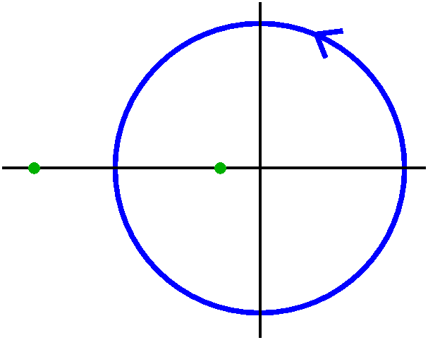
Deforming the integration contour continuously
The preliminary step is to distort the integration contour nicely. We
"distort" |z–a|=r as shown in the picture. Notice that the
distortions do not change the values of the line integrals since the
function we are integrating is analytic in A\{z}.
The integrals over the line segments connecting the two circles
cancel. We are left with integrals over two circles, one oriented
positively (in the usual, counterclockwise, direction) and the other
oriented negatively. Then Cauchy's Theorem implies that the integral
of g over |s–z|=r is equal to the difference of two integrals, one
over |s|=b and the other over |s|=a with r<a<|z|<b<R. Now
we handle each of the integrals. I'm just going to outline the process
-- it appears in virtually every complex analysis text. The
opportunity for making sign errors and summation index errors arises
frequently.
The outer integral
Well, consider
[1/(2Π i)]∫|s–z|=b(f(s)/(s–z))ds. We
will "expand the Cauchy kernel". So:
We know |s|=b>|z|, so 1/(s–z)=((1/s))(1/(1–[z/s])). Now we use the
geometric series, since |z/s|<1. The series will converge
absolutely for each such s. We can get nice error estimates just as we
did for the power series case. These estimates allow us to
"interchange" integration and summation. I won't bother with the
details of the estimates here.
The inner integral
Well, consider (1/2Π i)∫|s–z|=a(f(s)/(s–z))ds. We will "expand the
Cauchy kernel". So:
We know |s|=a<|z|, so
1/(s–z)=–((1/z))(1/(1–[s/z])). Now we use the
geometric series, since |s/z|<1. The series will consider
absolutely for each such s, and uniformly for s on |s–z|=a. Then we
interchange integration and summation.
A difficulty: convergence of doubly infinite sums
Before we state the result, think a bit about how
∑n=–∞∞qn should
be defined. One possibility is to look at
∑n=–NNqn and require
convergence as N→∞. This has some defects. For example,
then the double series with qn=–1 for n<0 and +1
for n>0 would converge (I guess to q0). This series
certainly would not converge absolutely, and the implication "absolute
convergence implies convergence" is useful and we should preserve
it. Also, if we used that definition, then relabeling n→n+1 might
change the sum of the series. So the more accepted definition is as
follows:
The series
∑n=–∞∞qn
converges and its sum is S if, given any real w>0, there is some
positive integer N so that if m1 and m2 are both
greater than N, then
|∑n=–m1m2 qn–S|<w.
Then the double series will converge if and only if each of the half
series (?), ∑n=0∞qn and
∑n=–∞0qn, converges,
and all of the expected statements will be correct.
Laurent Series Theorem
Suppose that 0≤r<R≤∞, and define an annular region A by
A={z in C with r<|z|<R}. Further, suppose that f is analytic in
A. Define the doubly infinite sequence of complex numbers
{an} by
an=∫|s–z|=t(f(s)/sn+1)ds
for any t with r<t<R. Then
- f(z)=∑n=–∞∞anzn
- This series converges absolutely for every z in A and good error
estimates can be gotten on any specific circle going around A.
- There is exactly one such series representing f in A.
- f can be written as a sum of fin, analytic in
{|z|<R}, and fout, analytic in {|z|>r}. This
decomposition is unique if also
limz→∞fout(z)=0.
Note
Replace z by z–p everywhere in all of those statements in order to
deal with an annulus centered at p.
Discussion of proof
Notice that in the formula for an, the integral
∫|s–z|=t(f(s)/sn+1)ds, there seems to
be a dependence on t. But Cauchy's Theorem declares that the result is
the same for all t with r<t<R.
The existence of the series is obtained by following the path of
expanding the Cauchy kernel twice, as mentioned before the statement
of the theorem. If there is such a series, then the coefficients can
be obtained by integrating f(s)/sn+1 around a circle, and
interchanging sum and integral using the error estimates which I have
refused to write! (Laziness or taste?)
Since Laurent series converge absolutely and we have good error
estimates, then any of the standard manipulations of algebra
(multiplication, addition, division, etc.) and calculus
(differentiation, integration) are justifiable, and any sort of
trickery which gets the series is justified.
fin is the sum of the non-negative z powers, and
fout is the sum of the negative z powers. The limit at
∞ means that the constant term, if non-zero, goes with
fin.
Examples
I will compute some Laurent series for rational functions.
For various reasons that will appear shortly, most other functions
have series which rarely can be computed explicitly.
 Let's consider the totally non-random rational function
R(z)=(4z2–14z+8)/(z3–10z2+32z–32). Written
that way I would have to work a bit to find series expansions. In
fact, I got this by combining some simpler (partial) fractions. It is
{1/(z–2)}+{3z/(z–4)2}. You can check this, hey, I won't do
it here after all, this is Math 403 and we
don't do the easy stuff. Maybe. I would like to find all possible
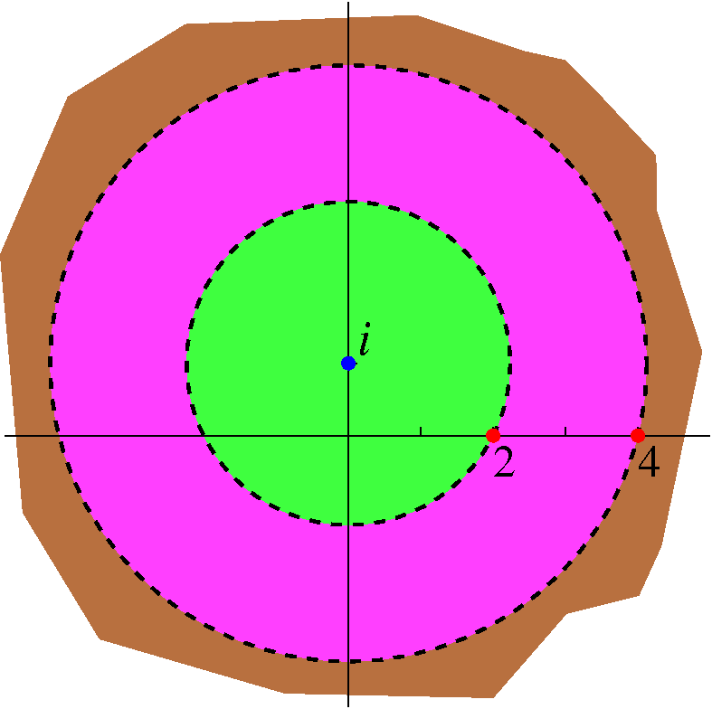
Laurent series centered at i for R(z). I note that R(z) is analytic
except for 2 and 4. And "clearly" there are three annuli
(plural of annulus, surely) centered at i in which R(z) is
analytic. These are
Let's consider the totally non-random rational function
R(z)=(4z2–14z+8)/(z3–10z2+32z–32). Written
that way I would have to work a bit to find series expansions. In
fact, I got this by combining some simpler (partial) fractions. It is
{1/(z–2)}+{3z/(z–4)2}. You can check this, hey, I won't do
it here after all, this is Math 403 and we
don't do the easy stuff. Maybe. I would like to find all possible
Laurent series centered at i for R(z). I note that R(z) is analytic
except for 2 and 4. And "clearly" there are three annuli
(plural of annulus, surely) centered at i in which R(z) is
analytic. These are
- |z–i|<sqrt(5) (which is the distance from i
to 2; this annulus is actually a disc)
- sqrt(5)<|z–i|<sqrt(17) (the distance from i
to 4)
- sqrt(17)<|z–i| (the only unbounded annulus
considered here)
We want series in powers (both positive and negative) of z–i. So we
need to write things in terms of z–i.
to be continued ...
| Monday,
March 29 | (Lecture #17) |
|---|
The primary task today is to "exploit" (use?) the Cauchy integral
formula for derivatives (CIFD) which we got by comparing two
descriptions of coefficients of power series. We will codify the
formula as the Cauchy estimates, and then find some wonderful
consequences.
 The Cauchy estimates
Suppose f(z) is analytic in some connected open set U which contains
the closed disc of z's with |z–a|≤r. Then for any non-negative
integer, n, |f(n)(a)|≤n!M/rn where M is the
maximum of |f(z)| on |z|=r.
Proof Suppose C is the boundary of the circle |z–a|=r with the
usual counterclockwise orientation. Then CIFD tells us that
f(a)=[n!/{2Πi}]∫C[f(z)/(z–a)n+1]dz. The
ML inequality gives us exactly the Cauchy estimate cited in
the statement of the theorem because L is 2Πr, so the Π's
cancel. Also |f(z)/(z–a)n+1|≤M/rn+1 if M is
as in the satement of the theorem. A power of r cancels so that we get
the rn in the bottom as the statement reads.
Probably the most interesting application of the Cauchy estimates is
the following which is really totally novel.
Liouville's Theorem
A bounded entire function is constant.
This strange result is easy to prove. If f is entire (analytic
everywhere in C), we'll show that f´(a)=0 if a is any
complex number. So we know that |f(z)|≤M for all z. The Cauchy
estimates, just for n=1, tell us that
|f´(a)|≤1!M/r1. But this is true for all r>0,
and the only non-negative number |f´(a)| which can satisfy these
inequalities is 0. So f´(a)=0 for all a's in C. The function is
constant!
This is an amazing result, which a friend in grad school with me
called the Louisville slugger because it is used many
circumstances where it totally cleans up the situation -- there are no
base-runners left. It has been difficult to explain this lovely pun to
some of our non-U.S. grad students. Your homework has a further
application, that if |f(z)| grows no faster than
(Constant)|z|n, then f(z) must be a polynomial of
degree≤n (so Liouville's Theorem is the case n=1).
Some counter(?)examples
With any new result, especially something so startling, exploring
possible counterexamples is always useful.
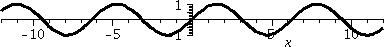 The function sin(z)
As we can see from the picture so generously supplied, this function
is not constant and is bounded by M=1. Explain that!
It ain't bounded as an entire function. You can easily when z=i y
and y is large positive, we've already shown that sin(z) is close to
i ey/2, an unbounded collection of numbers.
 The
function 1/(1+z2)
The
function 1/(1+z2)
This function is also surely bounded, and the bound is, again, as
displayed, 1. So it must be constant.
f is analytic but not entire, since z=±i is not
in the domain.
- The
function 1/(1+|z|2)
Now, since |z| is real and non-negative, I know that the domain of
this function is all of C! Again, surely this is a constant
function.
But f is not analytic. I think |z| is not complex
differentiable at any z, and actually |z|2 is complex
differentiable only when z=0, so |z|2 isn't analytic
anywhere. And don't call me Shirley.
Entire functions are very strange. For example, there is no
non-constant entire function whose image is inside the unit disc
(since such a function would certainly be bounded). And even more is
true. Near the beginning of the course we worked with
"simple" statements about complex numbers, modulus, complex conjugate,
etc. You had a few homework assignments which looked like this:
When is w=(z–i)/(z+i) inside the unit circle? Of course this asks:
when is ww<1? Let me
run through the elementary solution again. Observe that all the
steps are logical equivalences: they are reversible.
- Since (z–i)/(z+i) is (z+i)/(z–i), this is the same as
((z–i)/(z+i))·
((z+i)/(z–i))<1.
- This is the same as (z–i)(z+i)<(z+i)(z–i).
- Expanding, this means zz–iz+iz+1
<
zz+iz–iz+1
and we can clear away
the
zz and 1 from both sides.
- Push everything to one side and divide by 2. The result is
0<iz–iz.
- If z=x+i y, 0<iz–iz becomes exactly
0<i(x–i y)–i(x+i y) or –2i2y is positive or
just y=Im(z)>0.
So the mapping z→(z–i)/(z+i) takes the upper half plane to
the unit disc. It's inverse which is
w→(w–i)/(–iw–1) takes the unit disc to the
upper half plane -- the manipulations just gone through verify that
the algebraic inverse does do what I declare. In fact, we know:
Any entire function whose values are in the upper half plane is a
constant. For if it were not, then compose it with the mapping just
discussed (it sometimes has the name Cayley transform) and that
composition would have to be constant. But then compose this
composition with the inverse mapping and the result is the original
function, whose values are just one number. Thus the original function
must be constant.
Any entire function whose values are in the union of the first,
second, and third quadrants (those z's with 0<arg(z)<3Π/4)
must be constant. Hey: compose the function with the mapping
z→z2/3 which can certainly be defined in that
domain. It changes the 3/4 plane to the upper half plane (1-to-1 and
onto since z3/2 takes the half plane to the three quarters
plane!) and then the composition is constant by the previous
result. Etc.
These connected open sets make entire functions constant the range of
such a function is are inside them.
What's going on? Well, you'll need to wait just a little
bit more until we look at some geometry. First we have a major
result which is historically significant to check. I will approach the
result in a low-class (no: low-tech!) way.
Let me change gears and ask about a specific polynomial, let's say
P(z)=z4–(3+i)z3+9.22z+14.5. Maybe P(z) has
roots. If you do any sort of numerical work, an initial estimate is
always useful. Is there some circle |z|=R where it is
guaranteed that roots of P(z) must sit inside the
circle?
How BIG or how small is |f(z)| on a typical circle? Well,
certainly if P(z)=R≥1, then
|P(z)|=|z4–(3+i)z3+9.22z+14.5|≤|z|4+|3+i||z|3+9.22|z|+14.5≤AR4
where A=max(1,|3+i|,9.22,14.5). Also,
|P(z)|=|z4–(3+i)z3+9.22z+14.5|≥|z|4–|(3+i)z3+9.22z+14.5|.
But |(3+i)z3+9.22z+14.5|≤BR3 if
B=max(|3+i|,9.22,14.5).
In fact, if |z|=R≥2B, then
|(3+i)z3+9.22z+14.5|≤(1/2)R4 so that
|P(z)|≥R4–(1/2)R4=(1/2)R4.
Certainly P(z) has no roots if |z|>2B. These inequalities can be generalized.
If
P(z)=zn+∑j=0n–1ajzj,
then there is K>0 and positive constants C1 and
C2 so that for |z|≥K,
C1|z|n≤|P(z)|≤C2|z|n.
The following "constants" will work: C2 is just
max(1,|a0|,|a1|,...,|an–1|) with K at
least 1. C1 can be 1/2 but K needs to be greater than
2C2. So K=max(1,2C2).
This growth lemma (which essentially says, in theoretical computer
science language, |P(z)| has rate of growth |z|n as
|z|→∞ (sometimes written |P(z)}=Ω(|z|n)
when |z|→∞). This means |P(z)| can be estimated both above
and below by multiples of |z|n.
The Fundamental Theorem of Algebra
If
P(z)=zn+∑j=0n–1ajzj,
then there is at least one complex number a so that P(a)=0.
Once you know P(a)=0, then P(z)=(z–a)Q(z) where deg(Q)=n–1. So we can
continue to find roots, and write P(z) as a product of linear
factors.
Why is FTA true? Well, suppose that P(z) is never 0. Then
define f(z)=1/P(z), an analytic function whose domain is all of C
(entire!). I know that for |z|≥K,
|f(z)|<1/{C1|z|n} so
|f(z)|≤1/{C1Kn} for those z's. But |f(z)| is
continuous in |z|≤K so it has a bound, B, there (continuous
functions are bounded on closed and bounded sets). Therefore f(z) is
entire and bounded, hence (Liouville!) constant. But this is false
since P(z) is not constant. So P(z) must have a root.
Mr. Cantave commented that this "proof
by contradiction" wasn't totally useful -- it didn't come up with a
candidate or approximate candidate for a solution. Well, there are
other, constructive proofs. And, anyway, what does one expect in a
math class. This seemed to be an opportune time to tell my favorite
math joke, so I did.
JOKE
Several people are in a hot-air balloon, trying to land over a
fog-shrouded countryside at the end of a long day. The balloon dips
down low and they see the ground faintly. Spotting a person, one of
them calls down: "Where are we?" Some minutes later the wind is
carrying them away and they hear faintly, "You're in a balloon!" One
person in the balloon gondola says thoughtfully to the other, "It's so
nice to get help from a mathematician." The other says, "How do you
know that was a mathematician?" The first replies, "There are three
reasons: it took a long time to get the answer, it was totally
correct,
and, finally, it was absolutely useless."
The proof I just presented to you is one of the traditional proofs,
but, quick, before we discuss it, let me show you another
verification, this one due to Professor Anton Schep of the University
of South Carolina and published in 2009.
CIF applied to f(z)=1/P(z) at z=0 asserts that
2Πi/P(0)=∫unit circlef(z)/{z–0} dz=∫unit circle1/{zP(z)} dz. But we
can deform the unit circle: this integral has the same value as the
integral around a circle centered at 0 of radius R where R is large
(the integrand is analytic between these curves -- it only fails to be
analytic at 0). Then apply ML to
∫|z|=R{1/[zP(z)]} dz. We get
(2ΠR)/{RC1Rn} and this →0 as
R→∞. But 2Πi/P(0) isn't 0, so again, a contradiction and
we're done.
I think this is a sequence of lovely observations. It must be a nearly
minimal verification of FTA. It was published in A Simple Complex
Analysis and an Advanced Calculus Proof of the Fundamental Theorem of
Algebra, American Mathematical Monthly 116, Jan 2009, 67-68 by Anton Schep. The article is
available here.
FTA has a huge history and some special terminology. A field is
algebraically closed if every polynomial with coefficients in
the field has a root. A smaller field inside an algebraically closed
field has the bigger field as its algebraic closure if all
elements in the bigger field are needed to get roots of polynomials
with coefficients in the smaller field. So we have just proved that C
is algebraically closed, and that C is the algebraic closure of R. We
need the elements of C which aren't "real" in order to guarantee that
real quadratics have roots.
The history of FTA is complicated. There are books about FTA and
its history. On the web, here
is a comprehensive discussion of the history of the proofs. Another
discussion is here.
Probably FTA has hundreds of proofs. Many can be read here.
The doctoral dissertation of Gauss was about "a new proof of the
Fundamental Theorem of Algebra". Many authorities believe that what he
wrote then was actually the first credible proof of FTA,
although its own rigor has been criticized. Discussions of Gauss's
proofs (he gave 4 over his life!) are here
and here.
There's also a more practical question of actually approximating the
roots of a polynomial numerically: "constructive root finding". Anyone
who computes things worries about roots of polynomials. That's been
addressed in some of the references given above.
I further remark that FTA finally justifies (along with a lot of
linear algebra!) the method of partial fractions, taught and sometimes
learned (with much irritation!) in calc 2. Math is wonderful.
| Wednesday,
March 24 | (Lecture #16) |
|---|
When is ∫Cf(z) dz=0? Are such integrals
always equal to 0?
I will ask this question and hope to inspire some discussion and
investigation. Here are some answers which may occur.
- If f is analytic on and inside a simple closed curve C, then
the integral is 0. (Cauchy's Theorem).
- Not generally if f is not analytic, even if C is a simple
closed curve. Hey, try z on the unit circle.
- Not generally even if f is analytic and C is not a
closed curve. Try f(z)=z and C=[0,1].
- Not generally even if f is analytic on C and C is a
simple closed curve. Try 1/z on the unit circle -- this is exactly
what our noble ancestor Gauss means in this sentence extracted from the
long quote on the back of the fourth
homework assignment.
"If, for example, we define log x via ∫{1/x}dx
starting at x=1, then arrive at log x having gone around the point x=0
one or more times or not at all, every circuit adds the constant
+2Π i or –2Π i; thus the fact that every number
has multiple logarithms becomes quite clear."
So what if we just consider those C's which are simple closed curves
and we know somehow that all of the integrals of a function f(z)
around those C's are 0? This is enough to guarantee that f(z) is
analytic, even if you assume only that f(z) is initially
continuous. Differentiability then follows automatically. This
is amazing, and is useful in actual applications, as I will show
you. But first, let me state and prove a version of what's called
Morera's Theorem. There are many versions of this theorem, probably as
many as there are complex analysis textbooks, and this is only one.
Morera's Theorem
Suppose U is a connected open set and suppose that for all simple
closed curves C in U, ∫Cf(z) dz=0. Then f(z) is
analytic.
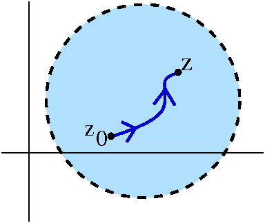 Proof Well, if I want to verify that f(z) is analytic, then it
is certainly enough to check that f(z) is analytic in an open disc
inside U. To the right is a picture of such a disc. I take some point
z0 in the disc (a fixed point -- it doesn't matter which
one) and I take any path P from z0 to a general point z. I
guess P should be piecewise differentiable, etc. Then I define
F(z) to be ∫Pf(z) dz. Here physics people might
recognize that choosing z0 is choosing a "ground state"
again. The value of F(z) does not depend on the choice of P, since the
"integral vanishing" hypothesis of Morera's Theorem implies that
f(z) dz is path independent.
Proof Well, if I want to verify that f(z) is analytic, then it
is certainly enough to check that f(z) is analytic in an open disc
inside U. To the right is a picture of such a disc. I take some point
z0 in the disc (a fixed point -- it doesn't matter which
one) and I take any path P from z0 to a general point z. I
guess P should be piecewise differentiable, etc. Then I define
F(z) to be ∫Pf(z) dz. Here physics people might
recognize that choosing z0 is choosing a "ground state"
again. The value of F(z) does not depend on the choice of P, since the
"integral vanishing" hypothesis of Morera's Theorem implies that
f(z) dz is path independent.
So now I'll verify that F(z) is (complex) differentiable, and that
F´(z)=f(z). The astute student (even a barely awake student!)
will notice that this is the third time I've done
this proof. What the heck -- this is such fun.
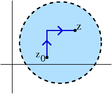 We can take a path as illustrated (ending with a horizontal line
segment) to compute F(z). Let me just look at the last part
carefully (with u(x,y) and v(x,y) being the real and imaginary parts
of f(z)):
We can take a path as illustrated (ending with a horizontal line
segment) to compute F(z). Let me just look at the last part
carefully (with u(x,y) and v(x,y) being the real and imaginary parts
of f(z)):
F(z)=∫vertical piecef(z) dz+∫x0xu(t,y)+i v(t,y) dt.
Here for the second piece, the horizontal part, I have parameterized
z=t+i y0 with t going from x0 to x,
z0=x0+i y0, and
z0=x+i y, Notice if I change x, the vertical piece of
the integral doesn't change. I can differentiate the formula with
respect to x using FTC of calc 1. The derivative is
u(x,y)+i v(x,y). By the way, if F(z)=U(x,y)+i V(x,y) is F's
decomposition into real and imaginary parts, we have just shown that
Ux=u and Vx=v.
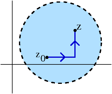 Here is the other picture we need (of course!). Now I've written a
path for which it will be easy to compute the y derivative of
F(z). So:
Here is the other picture we need (of course!). Now I've written a
path for which it will be easy to compute the y derivative of
F(z). So:
F(z)=∫vertical piecef(z) dz+∫y0y[u(x,s)+i v(x,s)]i ds.
Here in the second (vertical) part I parameterized by z=x+i s so
dz=i ds (don't forget the i!). s goes from y0
to y. Taking a y derivative uses FTC again, and the result on the
right is [u(x,y)+i v(x,y)]i which is –v(x,y)+i u(x,y). If
F(z) is U(x,y)+i V(x,y), then the left-hand side differentiates
to Uy+i Vy.
Let me summarize. We know this: Ux=u and Vx=v;
Uy=–v and Vy=u. What does this mean? Well, we
see that Ux=Vy and
Uy=–Vx. Therefore the real and imaginary parts
of F(z) satisfy the Cauchy-Riemann equations so we know that F(z) is
analytic. And the specific equations tell us that F´=f. But the
derivative of an analytic function is analytic, so f is also
analytic. We're done.
This is an amazing result because we got differentiability out of the
"machine" without any apparent effort (and we also got an
antiderivative for f(z), but that's not too helpful in practice!). I
will show how to use this in a second in a surprising way, but I
should observe that Morera's Theorem joins the previous catalog of
equivalent statements. I also "split" the power series statement into
two statements, one of which looks much "stronger" than the
other. They are equivalent to all the other statements.
A magical list
A remarkable fact which I've hinted at repeatedly but not explicified
(not a word!) is that a number of different characterizations
of functions are logically equivalent. This collection of results
leads to a very wide variety of tools to attack all sorts of
computational and theoretical problems. Suppose U is an open connected
set and f:U→C is a function. Here is what we know now:
- The definition
f has a complex derivative, f´(z), at each point z of U (this is
defined to be limh→0{f(z+h)–f(z)}/h) and f´ is
continuous. (Goursat showed that the requirement of continuity
can be dropped but I know no natural situation where the continuity of
f´ doesn't happen somehow automatically.)
- Power series I
f has a power series expansion valid near every point z0 of
U: that is, given such a point, there is a positive number r which
generally depends on z0 and a sequence of complex constants
{an}n≥0 so that the series
∑n=0&infinan(z–z0)n
converges for |z–z0|<r with its sum equal to f(z).
- Power series II
f has a power series expansion valid near every point z0 of
U: that is, given such a point, there is a positive number r which
generally depends on z0 and a sequence of complex constants
{an}n≥0 so that the series
∑n=0&infinan(z–z0)n
converges for |z–z0|<r with its sum equal to
f(z). The positive number r is at least the distance from
z0 to the boundary of U (because we can push out the circle
in the proof of the CIFD until it "hits" the edge of U).
- Differentiation
f has a continuous derivative f´ and this derivative also has a
continuous derivative.
- More derivatives
f has any number of continuous derivatives you may want (as long as
the number is at least 1 [sigh]).
- Cauchy-Riemann
If we write f as u+i v where u and v are real functions, then u
and v have continuous partial derivatives and satisfy the two partial
differential equations ux=vy and
uy=–vx.
- Harmonic functions
If the real part of f is u, then u is harmonic,
Δu=uxx+uyy=0, and the imaginary part of f
(that's v) is also harmonic and these two harmonic functions are
harmonic conjugates of each other.
- Morera's Theorem
f(z) is continuous, and for all closed curves C in U,
∫Cf(z) dz=0.
- A geometric characterization
This is called conformality and we'll get to it in a few weeks,
after we do a bunch of applications of what's already here.
|
Let me show you how to use this with a complicated computational
example. But first, a digression (!?) to calc 2. We have certainly
exploited many times the facts about geometric series which are
reviewed in calc 2 (after being learned, maybe, in either high school
or junior high). Another family of series is studied in calc 2.
p-series
The p-series is the series
1+1/2p+1/2p+1/3p+1/4p+...
(etc.). You may remember that this series converges when p>1. It
has to converge absolutely since the series consists of
positive terms. How fast does it converge? Let me recall some of calc
2, and let me temporarily concentrate on p=2. Now
∑n=1∞1/n2=∑n=1N1/n2+∑n=N+1∞1/n2.
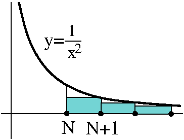 How big is the "infinite tail",
∑n=N+1∞1/n2?
How big is the "infinite tail",
∑n=N+1∞1/n2?
The standard calc 2 technique for estimating this sum is to compare it
to an integral. I always get confused about this, but a picture
helps. The boxes are under the curve y=1/x2, and so
the infinite tail is less than
∫N∞[1/x2]dx. But I can find
exact antiderivatives of powers, and then plug things in. The value of
this improper integral is 1/N. So the tail
∑n=N+1∞1/n2 is less than
1/N. By the way, more numerical work shows that this is about as good
as you can expect. The tail can't be estimated much better than
this asymptotically.
What if I wanted to know for which N the partial sum will be within
.001 of the value of the whole sum? Well, .001 is 1/1,000 so I would
need a thousand terms. By contrast, if we look at the geometric series
∑n=1∞1/2n, the
corresponding tail
∑n=N+1∞1/2n is exactly
1/(2N). To get accuracy of .001, I would just need
N=10. Or, another way, if I took N=100, I'd get accuracy of ... uhhh
... less than 8·10–31, which seems small. These p-series converge much slower than
geometric series.
What if I vary the p? If I make p larger than 2, then the
terms get smaller (1/np decreases as the positive real
number p increases). So in fact I get an error of <.001 by taking
at least 1,000 terms for any p-series with p≥2.
Complex p-series?
Remember that ab=eb log(a) with
log(a)=ln(a)+i arg(a). Here I will take a to be a positive integer
n, and b will be z=x+i y. Also since n is a positive real, let me
just use the principal branch of log, so Arg(n) is 0. Now
nz=e(x+i y)ln(n)=ex ln(n)e(i y)ln(n).
The modulus of np is exactly
ex ln(n)=nx since
ei (any real) has modulus 1. So |1/nz|
is just e–ln(n)Re(z)=1/nx. Therefore the
modulus of ∑n=1∞1/nz will
converge absolutely if x=Re(z)>1 because I can compare the
terms to terms of the usual p-series with p=Re(z).
The series ∑n=1∞1/nz
converges absolutely and therefore converges in the open half-plane
Re(z)>1. I will temporarily call this sum Q(z). What sort of
function is it? In fact, I claim this sum is actually an analytic
function. Please note that verification of this by, say, using the
definition is not so easy. The examples I showed you of Fourier series
where the sum of the derivatives is not the derivative of the sum
should perhaps suggest that. This series is not a power series,
and it is much worse (converges much slower) than such a series. We
should be careful even though each piece,
1/nz=e–ln(n)z, is easily seen to be
analytic (just differentiate with the Chain Rule!). So I'll be a bit
cute here and use Morera's Theorem.
 If I took, say, z's with Re(z)≥2, I know that
Q(z)=∑n=1N1/nz+Error(N) where
Error(N) is a complex number and |Error(N)|<1/N. This is because
any such series can be overestimated by the ordinary p-series with p=2
and the infinite tail can be overestimated by the same estimate of the
usual infinite tail. Now suppose C is a simple closed curve of length
L in the half plane Re(z)≥2. Then:
If I took, say, z's with Re(z)≥2, I know that
Q(z)=∑n=1N1/nz+Error(N) where
Error(N) is a complex number and |Error(N)|<1/N. This is because
any such series can be overestimated by the ordinary p-series with p=2
and the infinite tail can be overestimated by the same estimate of the
usual infinite tail. Now suppose C is a simple closed curve of length
L in the half plane Re(z)≥2. Then:
∫CQ(z) dz=∫C∑n=1N1/nz dz+∫Cinfinite tail dz
Each of the pieces 1/nz in the finite sum is analytic and
therefore (Cauchy's Theorem)
∫C∑n=1N1/nz dz=0.
What about ∫Cinfinite tail dz? We estimate
its modulus using ML. The M is 1/N so this piece has modulus less than
L/N. But we can do this for any N. This means that the modulus
of the integral we started with, ∫CQ(z) dz, is
less than L/N for any positive integer N. There is only one
non-negative number like that: 0. So the integral over C of Q(z) is 0.
The p=2 restriction is sort of silly, and we could do any p>1
similarly. The function Q(z) is actually analytic in Re(z)>1.
What's going on?
I haven't told you the REAL NAME of
this function.
The letter ζ is a Greek letter zeta, and this is the Riemann zeta
function, one of the most famous functions in mathematics.
For more general background about this function, see here
or here.
The second reference states that this function "plays a pivotal role
in analytic number theory and has applications in physics, probability
theory, and applied statistics." If you study this function and learn
a lot about it, maybe you can make a
million dollars. The connected between the zeta function and prime
numbers uses the Euler infinite product (here is a
statement and a proof of the formula -- the proof is not the one
I'm used to).
| Monday,
March 22 | (Lecture #15) |
|---|
The Cauchy Integral Formula for Derivatives
Suppose R is a connected open set, C is a simple closed curve whose
inside is contained entirely in R, p is a point inside C, and f is
analytic in R. Then for any positive integer n, f is n times
differentiable, and f(n)(p)={n!/[2Π i]}∫C[f(z)]/[(z–p)n+1]dz.
I think I proved this only for a circle which has p inside it, but any
C described in the theorem can be deformed to such a circle, so the
result is true also. I will try to substantiate this by drawing an
appropriate picture such as the one to the right, which I've already
drawn once. For this change, though, just reverse the arrows: make the
circle into C. Notice that the integrand,
[f(z)]/[(z–p)n+1], is analytic in all of the region
except for p so this deformation does not change the value of
the integral. | 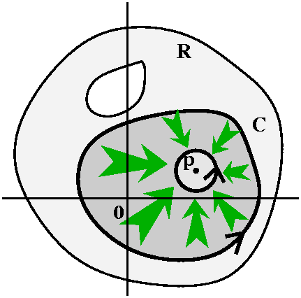 |
 A strange estimate on the size of derivatives
If you really believe in the CIF for derivatives, then very strange
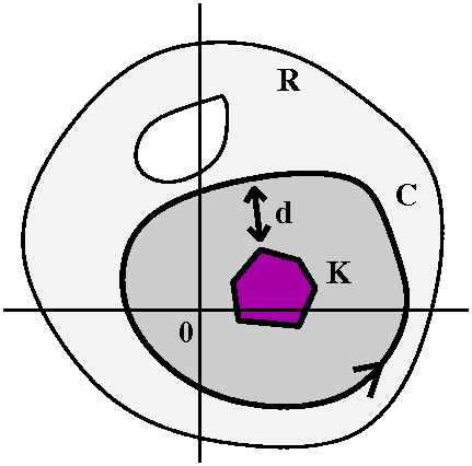
things happen. Let me show you. Suppose we take C as above inside a
connected open set R, and the inside of C is entirely inside R, as
shown. Suppose all of our p's are in a set K and all the p's are at a
distance at least d to the curve C. So the setup is sort of what is
pictured to the right. Now I know that if p is any point in K,
f(n)(p)={n!/[2Π i]}∫C[f(z)]/[(z–p)n+1]dz.
Let me apply the ML inequality in a very direct way. The length of C
will be L. And I want to estimate the modulus of the integrand,
[f(z)]/[(z–p)n+1]. Let me label the maximum of the
modulus of f(z) on C with M. I need to underestimate |z–p| where
z is on C and p is in K. Well, certainly one underestimate is d. I am
not going to get anything very precise because I haven't given you
very much specific information. We get this sort of result:
If p is in K, then
|f(n)(p)|≤{n!/[2Π]}CM/dn+1.
Now I don't want to beat this inequality to death (that will occur
next time, when you'll see it is even more weird than it seems today)
but notice the M on the right-hand ("upper") side. If M gets very very
small, so the modulus of the function is tiny, this inequality
declares that the derivatives inside must also get very very small. So
a small function (in the sense of modulus) implies small derivative
(in the sense of modulus). Derivatives sort of control the amount of
wiggling in a function, and this means that very small functions
can't wiggle very much. Understand?
 A counter(?)example(?)
The best examples I know of in math are the ones which force you to
reconsider your assertions, or, at least, to look very closely at
them. Look now at the sequence of functions {sin(n2x)/n}
where n is a positive integer. Certainly these functions are bounded
(their values are in the interval [–1/n,1/n]). As
n→∞, certainly the sizes (maximum heights of these
functions) →0. But, wait: their derivatives are
n cos(n2x), and certainly these functions, the first
derivatives, get really really big as n→∞ (the values
occupy all of [–n,n]). There is a great deal of wiggling going
on. (That's 3 certainly's, so everything should be totally
clear [NO!].)
What is happening?
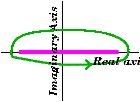 Of course the answer is that the complex sine is not
bounded at all away from the real axis. We should really look at the
complex picture. We need a closed curve around a piece of the
real axis. To the right is shown such a curve, C, around a chunk of
the real axis. Notice that the curve crosses the imaginary axis at two
places.
Of course the answer is that the complex sine is not
bounded at all away from the real axis. We should really look at the
complex picture. We need a closed curve around a piece of the
real axis. To the right is shown such a curve, C, around a chunk of
the real axis. Notice that the curve crosses the imaginary axis at two
places.
Remember that if y is real, sin(i y)=i sinh(y), and
sinh(n2y) is exactly
{en2y–e–n2y}/2. The second
piece if y is positive →0 rapidly as n→∞. But for
fixed non-zero positive y, sinh(n2y) is like
en2y/2 for n large. It grows really, really
fast! So both the example and the previous estimate (which will return
shortly in a form called the Cauchy estimates) are correct but
they essentially have little to do with one another. What happens on
the real axis to an analytic function is not a complete qualitative
description of the behavior of the function.
A magical list
A remarkable fact which I've hinted at repeatedly but not explicified
(not a word!) is that a number of different characterizations
of functions are logically equivalent. This collection of results
leads to a very wide variety of tools to attack all sorts of
computational and theoretical problems. Suppose U is an open connected
set and f:U→C is a function. Here is what we know now:
- The definition
f has a complex derivative, f´(z), at each point z of U (this is
defined to be limh→0{f(z+h)–f(z)}/h) and f´ is
continuous. (Goursat showed that the requirement of continuity
can be dropped but I know no natural situation where the continuity of
f´ doesn't happen somehow automatically.)
- Power series
f has a power series expansion valid near every point z0 of
U: that is, given such a point, there is a positive number r which
generally depends on z0 and a sequence of complex constants
{an}n≥0 so that the series
∑n=0&infinan(z–z0)n
converges for |z–z0|<r with its sum equal to f(z).
- Differentiation
f has a continuous derivative f´ and this derivative also has a
continuous derivative.
- More derivatives
f has any number of continuous derivatives you may want (as long as
the number is at least 1 [sigh]).
- Cauchy-Riemann
If we write f as u+i v where u and v are real functions, then u
and v have continuous partial derivatives and satisfy the two partial
differential equations ux=vy and
uy=–vx.
- Harmonic functions
If the real part of f is u, then u is harmonic,
Δu=uxx+uyy=0, and the imaginary part of f
(that's v) is also harmonic and these two harmonic functions are
harmonic conjugates of each other.
- Morera's Theorem
I'll discuss this very shortly but it links path independence to all
the other characterizations.
- A geometric characterization
This is called conformality and we'll get to it in a few weeks,
after we do a bunch of applications of what's already here.
|
I will try to persuade people that we actually know that all of these
characterizations are equivalent already, and that we know even more
(e.g, the Cauchy integral formula for derivatives ties together
integrals of f and the coefficients of the various power series
expansions of f). Let me show you some very slick applications of
these equivalent statements (just a few -- most of the remainder of
the course will be such applications!).
Steady state heat flows aren't kinky
In physics and certain other areas of applications, people study
harmonic functions as a key part of the mathematical model of their
discipline. For example, a solution u of Δu=0 might be a
steady-state heat flow, or it might be an electromagnetic field away
from a charge or ... lots of things. A very similar differential
equation is the Wave Equation, which is
uxx–uyy=0. The phenomena which are
modeled by the Wave Equation include things like sound and other
vibrations. The solutions of the Wave Equation characteristically (a
bit of a joke, that word, if you've had a PDE course!) have breaks or
shocks -- the mathematical counterpart of what we can see visibly in
vibrations and other phenomena. But if we change – to
+, here is what happens:
Suppose we have uxx+uyy=0. Pick any point p and
any disc centered at p in the domain of u. In lecture #10 on February
22, we brute force "created" a harmonic conjugate v for u just in that
disc. The proof was yucky, but the fact was verified. So there is v so
that u+i v is analytic. I am not declaring that ALL of u has a
harmonic conjugate, since in the same lecture I gave an example of a u
without a harmonic conjugate. But "locally" I can always find one. Now
f=u+i v can be differentiated any number of times. So therefore u
can be differentiated also. Therefore, any harmonic function,
assumed only twice differentiable in its definition, is actually
infinitely often differentiable! Heat flow has no shocks.
This is not an obvious conclusion.
 But there really are kinky (very weird) functions!
Almost all of the ideas covered in this course are mathematics which
was created and maybe nearly perfected in or before the
19th century. So perhaps I should look a little bit
forward, and tell you what wasn't well known to professors in
1850. The specific example I'm about to discuss also shows some of the
power in what we have already proved. So here is (nominally!) an
example from calc 1.
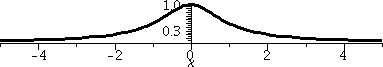
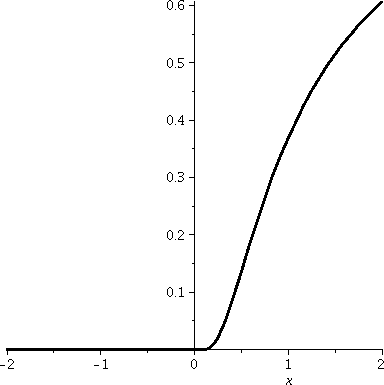
Consider the function f:R→R defined piecewise by f(x)=0 for
x≤0 and f(x)=e–1/x for x>0. A Maple graph of this function is shown to the
right.
The difficulties in this function occur at/near x=0. For x>0, the
value e–1/x is
exp(a negative number). Therefore, if x>0,
0<f(x)<1. In fact (we are "in" calc 1 mode) for x>0,
f´(x)=e–1/x(1/x2). This function is
positive for all x>0, so f(x) is increasing for
x>0. Also, note that
limx→∞e–1/x=1 because when x is
large positive, –1/x is small positive, so
exp of that is close to 1. Also,
limx→0+e–1/x=0. Why? If x
is small and positive, then –1/x is large and negative, and exp
of that is close to 0. In fact, we have just verified that f(x) is a
continuous function for all values of x. This is "obvious" for
x<0 and for x>0 (there f(x) is given by a nice formula). The
only value we really need to check is at x=0: we just did this.
What may not be clear is differentiability of f(x). If x<0, sure it
is, and I bet that f´(x) is 0 for those x's. If x>0, I know
that f´(x) exists and is actually given by the wonderful formula
f´(x)=e–1/x(1/x2). Again, the difficult
"point" is x=0. We need to study
limh→0[f(0+h)–f(0)]/h. Well, if h<0 the top is
(0–0)/h which is 0. So we need to check that
limh→0+[f(0+h)–f(0)]/h exists and is
0. Now f(0)=0 (that's in the darn definition!). And for h>0, f(0+h)
is e–1/h. So we need to "compute"
limh→0+e–1/h/h. A few
people remembered the contortions (?) which are needed to compute
this. Here is how to do it.
To compute
limh→0+e–1/h/h, change
variables: let's call 1/h the new variable w. Then
what does "h→0+" turn into? If h is small and positive, then w
is large and positive. And e–1/h/h becomes e–ww,
so that the limit turns into
limw→∞e–ww=limw→∞w/ew.
This limit, finally, can be computed with L'Hopital, and we
differentiate the top and bottom to get the limit of 1/ew
as w→∞. This limit is easily equal to 0.
Wow. We have just used only a sort of simple-minded analysis to, in a
"brute force" way, show that f is differentiable at x=0, and that
f´(0)=0.
So we have a description of f´. Here it is: f´(x)=0 for
x≤0 and f´(x)=e–1/x(1/x2). What is more
amazing is that this function is, in turn, differentiable. For x<0,
of course f´´(x)=0. For x>0, if I use the Chain Rule and
the Product Rule correctly (which I didn't in class!) then
f´´(x)=e–1/x({1/x4}–{2/x3}).
What happens at x=0? Again, we think of a two-sided limit, and the
left-hand limit is just 0. Therefore we need to consider
limh→0+{f´(0+h)–f´(0)}/h. This
becomes
limh→0+e–1/h(1/h3)
using the known value of f´(0) (that's 0) and the formula for
f´(x) when x>0. The same trick as before (1/h becomes w etc.)
turns this limit into
limw→∞w3e–w. Well, we
think of w3/ew and use L'Hop three times. Etc.
Etc. indeed!
It turns out (o.k., darn it, a proof using mathematical induction)
that f can be differentiated infinitely often (any number of times)
and that for any positive integer n, f(n)(0) is 0. The
graph of y=f(x) is flat, really flat, infinitely flat (!) at
the origin. This is a bit distressing because of the following
statements.
- The Taylor series for f centered at x=0 is ... 0. (Yes it is! All of the coefficients are 0.)
- The radius of convergence of the Taylor series of f centered at
x=0 is ∞ (well, darn it, the series does converge for every x).
- There is no interval centered at x=0 for which f(x) is
equal to its Taylor series centered at 0.
The situation in complex analysis is actually much simpler than the
situation in real calculus. In real calculus, very strange things can
happen to functions: sometimes 15 derivatives can exist and sometimes
not. Sometimes infinitely many derivatives exist, but sum of the darn
Taylor series can have nothing to do with the original function. That
can't occur in complex analysis.
| Wednesday,
March 10 | (Lecture #14) |
|---|
 Deforming curves but not changing the value of line integrals
Here is a more complicated corollary of Cauchy's Theorem. It will allow
us to compute many more integrals by comparing them with one another.
Corollary
Suppose that f(z) is analytic in a region R, and that
C1 and C2 are simple closed curves in R. Suppose
also that the curves can be continuously deformed, one into the other,
all inside the region R. Then
∫C1f(z) dz=∫C2f(z) dz.
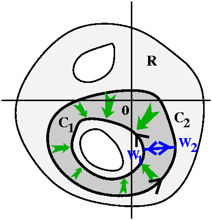
About the picture The picture attempts to illustrate the
situation described in the corollary. The region R is a connected open
set. The green arrows show how the curve
C2 is deformed into C1 through part of R
(but not through any of the holes!). If we picked a point
w2 on C2, the deformation would move it along a curve to a point w1 on
C1: let's call that curve B.
Proof Look at this curve, which is a sum of curves: start at
w2 and move along C2 until we get to
w2 again. Then move on B until we arrive at
w1. Now move backwards on C1, returning
to w1. Finish by moving backwards on B. The curve described
is C2+B–C1–B. We apply Cauchy's Theorem to that
curve, because f(z) is analytic on and inside the curve. The integral
is 0, but that means 0=∫C2+B–C1–Bf(z) dz=∫C2f(z) dz+∫Bf(z) dz–∫C1f(z) dz–∫Bf(z) dz, so (since the B integrals cancel) we get
∫C1f(z) dz=∫C2f(z) dz.
Comment Here is some (negative) discussion about this
"proof". What do I mean precisely by "deformation"? I haven't
described this. Well, the notion can be described precisely, but I
won't do it in this course, and in any situation I use this result in
this course will be one where a picture verifying the proof can be
explicitly drawn. Another objection can be applying Cauchy's Theorem
to the curve C2+B–C1–B. This really isn't a
simple closed curve. Again, this is true, but it is a limit of
simple closed curves (think of twin B's slightly separated, with
accompanying twin w2's and w1's). Each of those
curves would be simple closed curves, and each would have integral
equal to 0. The limiting curve with limiting integral would then also
have integral equal to 0. The idea is what I'm showing here, and I am
willing to admit that I've given up some precision!
The one non-zero integral we need ...
We know that ∫|z|=1(1/z)dz=2Π i. This is a
vital fact. (You can compute this directly using z=eit
etc.)
| 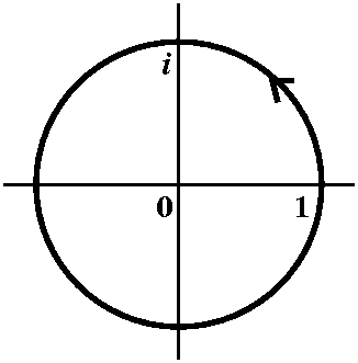 |
A strange choice of function
 What I'm describing is a somewhat complicated setup. I don't think
I'll make it better by declaring that the whole procedure is one which
is used repeatedly in many areas of applied mathematics, engineering,
and physics. I will try, though, to describe the simplest incarnation
of the situation. So here are the ingredients:
What I'm describing is a somewhat complicated setup. I don't think
I'll make it better by declaring that the whole procedure is one which
is used repeatedly in many areas of applied mathematics, engineering,
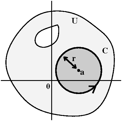
and physics. I will try, though, to describe the simplest incarnation
of the situation. So here are the ingredients:
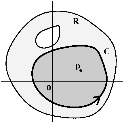
- A connected open set R and a function f(z) which
is analytic in R.
- A simple closed curve C whose inside is contained entirely in R.
- A random (!) point p inside C.
Now I want to consider the function g(z)=[f(z)–f(p)]/[z–p]. This is
sort of bizarre, but stay with me. This function is certainly analytic
everywhere that f is analytic, except perhaps at p. Because of the
division by z–p, we can't be sure about the formula's behavior at
p. So everywhere except p (and inside R) g(z) is surely
analytic.
Now let's consider a very small circle centered at p, all inside the
curve C, as shown in the picture. The curve C can be deformed
to the small circle through points in R which are not p. But g is
analytic at those points, so the integral doesn't change. That is,
∫Cg(z) dz=∫small circleg(z) dz.
Now we'll compute ∫small circleg(z) dz. Let's
suppose the circle has radius r. Of course we know that the modulus of
the integral is bounded by ML, where L is 2Π r and M is the
maximum of |g(z)| on the circle. But the formula for g(z) is not
random. It is the difference quotient defining the derivative of f(z)
at p. That means limz→pg(z)=f´(p). More
specifically, the limit statement itself means this: given
ε>0, there is δ>0 so that when
0<|z–p|<δ then |g(z)–f´(p)|<ε. That
is, g(z)=f´(p)+error where |error|<ε. So for small r (any r less
than δ) we know that |g(z)|<|f´(p)|+ε which we can take as
M. The integral of ∫small circleg(z) dz
therefore has modulus less than (2Π r)(|f´(p)|+ε). Let me be
more precise by stating this carefully:
∫small circleg(z) dz doesn't depend on the
radius of the small circle, and, given any ε>0, when the radius r
is small, the value of the integral's modulus is at most
(2Π r)(|f´(p)|+ε). But that estimate can be made as small as you
like by taking r very small. The only way the estimate can be correct
is if the value of the integral itself is 0.
Therefore ∫small circleg(z) dz=0. But let's write in
the formula for g, so this becomes
∫small circle[f(z)–f(p)]/[z–p]dz. Break up the
fraction in the integrand, so we get ∫small circle[f(z)]/[z–p]–[f(p)]/[z–p]dz and
this is further ∫small circle[f(z)]/[z–p]dz–∫small circle[f(p)]/[z–p]dz. The second
integral is ∫small circle[f(p)]/[z–p]dz=f(p)∫small circle1/[z–p]dz
because f(p) is a multiplicative constant with respect to integration
by z. And, finally, ∫small circle1/[z–p]dz is 2Π i, the only
integral we'll ever need. So
∫small circleg(z) dz=0 becomes
∫small circle[f(z)]/[z–p]dz–2Π f(p)=0. But
the integral of f(z)/[z–p] over C is the same as the integral of
f(z)/[z–p] over the small circle. We've just verified a major result
of the subject.
The Cauchy Integral Formula
Suppose R is a connected open set, C is a simple closed curve whose
inside is contained entirely in R, p is a point inside C, and f is
analytic in R. Then f(p)={1/[2Π i]}∫C[f(z)]/[z–p]dz.
Comment This is a fundamental and remarkable
result. Differentiability, that is, complex differentiability,
has the consequence that knowing the values of f on C determines the
values of f inside C. We need to sort of "average" the values
properly with weights determined by 1/[z–p] but everything is
determined by the boundary values. This has no counterpart in real
calculus. Certainly a differentiable function's value inside an
interval is not determined by what happens at the endpoints of the
interval.
An example and exercise: a trig integral
I asked Maple to compute
∫02Π1/[3+sin(t)]dt and the response I got
was Πsqrt(2)/2. Let me show you one way this can be done. I will
use complex analysis and the Cauchy integral formula. There are short
cuts we will develop in the next few weeks, but I want to present you
with a cute direct application of CIF (the Cauchy integral formula).
I will "reverse engineer" the transformation which we've done many
times in this course, where we started with a line integral and then,
by parameterization, got a standard definite integral. Here we will
start with ∫02Π1/[3+sin(t)]dt. Certainly
the bounds 0 and 2Π on the definite integral suggest "the unit
circle" to me, so z=eit and 0≤t≤2Π. Then
dz=i eitdt so that dz/(i eit)=dt and
dz/(i z)=dt. But I need to know how to change sin(t) into
"z-land". Here my knowledge of power series helps, and I remember that
sin(t)=[eit–e–it]/2i=[z–(1/z)]/2i. Now the
integral we started with becomes:
∫|z|=1(1/[3+{z–1/z}/2i]((dz/iz)=∫|z|=1(2/(z2+6i z–1))dz.
That's if I did the algebraic "massage" of the integrand
correctly. Now where is the integrand analytic? Well, everywhere
except at the roots of z2+6i z–1. The Quadratic
Formula applies here (it is a problem in one of the first sections of
the book, but, actually, the Quadratic Formula applies in any
field). The roots are: [–6i±sqrt{(–6i)2+4}]/2. Under
the square root we have (–6i)2+4=–36+4=–32. We divide
everything by 2 (by 4 under the square root!) and get as roots (–6±2sqrt(2))i. Well,
r1=(–6–2sqrt(2))
i is inside the unit circle and r2=(–6+2sqrt(2)) i is outside the
unit circle. But the integral we have is
∫2/[(z–r1)(z–r2)]dz. This is exactly CIF with f(z)=2/(z–r2) and
p=r1, and therefore the value of the integral is
2Πi f(r1) which is
4Πi/(r1–r2) which turns out to be ...
4Πi/(4sqrt(2)i), the same as Maple's
Πsqrt(2)/2.
 Expanding the Cauchy kernel
The Cauchy kernel is the function 1/[z–p]. It can be
manipulated algebraically in a variety of ways to give properties of
analytic functions. I'll do a basic example of this manipulation
here. Later we will do others.
I will suppose f(z) is analytic in some big disc centered at 0. For my
simple closed curve I will take a circle of radius R centered at
0. The radius will be smaller than the radius of the "big disc". Also
p will be some point inside the circle of radius R. Then I know
f(p)={1/[2Π i]}∫|z|=R[f(z)]/[z–p]dz. Consider 1/[z–p]. Since z is
on |z|=R and p is inside the circle, |p|<R=|z|. |p/z| is less than
1. So do this:
1/[z–p]=[1/z]/[1–{p/z}]: this is supposed to make you think of the
formula for the sum of a geometric series, a/[1–r], since we have
arranged for r to be p/z, a complex number of modulus less than 1. We
could write the whole infinite series, or just stop after a few
terms. Let me show you.
[1/z]/[1–{p/z}]=∑n=0∞pn/zn+1=∑n=0Npn/zn+1+∑n=N+1∞pn/zn+1=&sumn=0Npn/zn+1+[pN+1/zN+2]/[1–{p/z}].
Here the ERROR, the difference between
the partial sum and the whole series, is
[pN+1/zN+2]/[1–{p/z}]. The modulus of this is at
most (for any z on the circle)
[|p|N+1/RN+2]/[1–{|p|/R}] and since |p|/R<1,
ERROR→0
as N increases.
Now let's stuff the preceding sum into the integral:
∫|z|=R[f(z)]/[z–p]dz=∫|z|=R[f(z)](∑n=0Npn/zn+1+ERROR)dz
The finite sum is really
∑n=0N∫|z|=R[f(z)]
pn/zn+1dz=∑n=0N(∫|z|=R[f(z)]/zn+1dz)pn.
The other term can be estimated by ML: the length is 2Π R while the M is the maximum of |f| on the circle |z|=R multiplied by [|p|N+1/RN+2]/[1–{|p|/R}]. Since
|p|/R<1,
this will go to 0 as N increases. But put everything together. We have just shown that a certain infinite series converges, and since we know the Cauchy integral formula, we also know the sum of the infinite series.
f(p)=∑n=0∞anpn where
an=[1/{2Π i}]∫|z|=R[f(z)]/zn+1dz.
Complex differentiability implies power series
Here is a general statement of the preceding result.
Theorem Suppose f(z) is analytic in a connected open set which
includes some disc centered at a point z0. Then there are
complex numbers {an}n=0∞ so that the series ∑n=0∞an(z–z0)n converges at
least for all z in that disc centered at z0. Additionally,
the coefficients an are given by the formula
an=[1/{2Π i}]∫|z–z0|=R[f(w)]/(w–z0)n+1dw
where R is any positive number less than the radius of the disc.
Consequences
First, since power series can be differentiated inside their
radius of convergence, we see that a complex differentiable function
has a derivative which is itself a complex differentiable function!
This is totally unlike real calculus. For example, we know that |x|
can't be differentiated at 0. It has an antiderivative, let's call it
h(x), given piecewise by x2/2 for x>=0 and by
–x2/2 for z<0. The function h(x) has a derivative (just
|x|) and it does not have a second derivative. In the complex "realm",
functions always have more derivatives! There aren't any problems like
|x|. One derivative implies having infinitely many derivatives!
Second, we saw when we studied power series that a function can
have only one power series representation centered at a point. That
is, if f(z)=∑n=0∞an(z–z0)n and
f(z)=∑n=0∞bn(z–z0)n, both
converging near z0, then each an is equal to the
corresponding bn. In fact, since we can differentiate power
series, the power series must be a Taylor series:
an=(1/n!)f(n)(z0). But we can compare
the two descriptions of the coefficients an we have, and
then we can deduce the following result.
The Cauchy Integral Formula for Derivatives
Suppose R is a connected open set, C is a simple closed curve whose
inside is contained entirely in R, p is a point inside C, and f is
analytic in R. Then for any positive integer n, f is n times
differentiable, and f(n)(p)={n!/[2Π i]}∫C[f(z)]/[(z–p)n+1]dz.
I think I proved this only for a circle which has p inside it, but any
C described in the theorem can be deformed to such a circle, so the
result is true also.
| Monday,
March 8 | (Lecture #13) |
|---|
I handed out copies of some pictures
and supporting discussion about trigonometric series. Here's a web
version of the same material.
Here are graphs of the partial sums of some trigonometric series.
If w is real, then |sin w|≤1 so the infinite series
∑j=1∞sin(2jx)/j5
converges for all x because it converges absolutely. An easy estimate
with an improper integral
(∑j=51∞(1/j5)<∫j=50∞dx/x5)
shows that the partial sum of the first 50 terms is within .00000004
(yes!) of the whole sum.
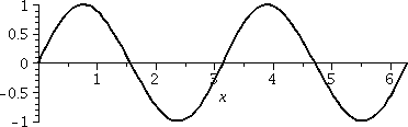 Here is a Maple graph of the partial sum
∑j=150sin(2jx)/j5 on the interval
[0,2Π]. Humans would not notice any discrepancy as small as what
was just written. I think the graph of the entire series
would look the same -- for the scale displayed!
Here is a Maple graph of the partial sum
∑j=150sin(2jx)/j5 on the interval
[0,2Π]. Humans would not notice any discrepancy as small as what
was just written. I think the graph of the entire series
would look the same -- for the scale displayed!
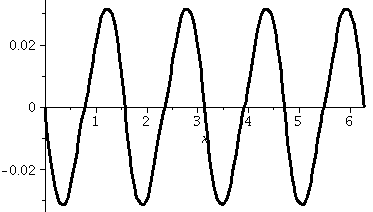
|
And, by the way, the graph is not the graph of sin(2x) (I
worried about that also!). A graph of the difference is shown to the
left, with vertical range about [–.03,.03]
|
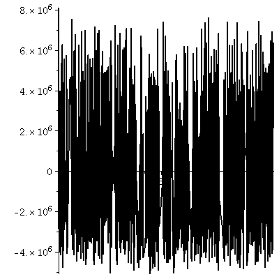
Now here is a Maple graph of
∑j=1502jcos(2jx)/j5,
a partial sum of a much stranger trig series. I just differentiated
each term in the partial sum of the first series and added the
results. Notice that the graph is emphatically not nice!.
The interval of x's is again [0,2Π] but Maple has scaled the vertical axis. It is
about [–5·106,8·106]. The
graph isn't reliable here because of the difficulties of plotting a
function with such wiggly behavior.
The series
∑j=1∞2jcos(2jx)/j5
probably doesn't converge very often. For example, suppose
x=Π/2k for some positive integer, k. Then as soon as the
index of summation, j, passes k, the cosine function is evaluated at a
multiple of 2Π so the terms of the series are
2j/j5, which does not →0, Many other
x's have similar or even more bizarre properties. Therefore the
term-by-term derivative of the original series does not converge.
I am not asserting that the original series is not
differentiable (its sum is actually yet another "special function"
which Maple identifies and can
differentiate). I do assert that the simple generalization of "The
derivative of a sum is the sum of the derivatives" to an infinite
series is false in this case. Power series are very
nice. Trigonometric series are not.
So here is what some of the niceness causes: a few consequences of the
third statement about power series:
Suppose R≠0. Then the sum of the series
&sumj=0∞aj(z–z0)j,
inside the radius of convergence (that is, for
|z–z0|<R). is a complex differentiable function
whose derivative is the sum of the series
&sumj=0∞j aj(z–z0)j–1
which has the same radius of convergence.
This says that a power series can be differentiated, and that its
derivative is equal to the sum of a series of differentated terms, and
that latter series has the same radius of convergence. .
Suppose
f(z)=&sumj=0∞aj(z–z0)j.
Then f(z0)=a0 because all of the other terms
drop out (z0–z0=0).
Let's differentiate:
f´(z)=&sumj=0∞j aj(z–z0)j–1.
Now "plug in" z0. The result is
f´(z0)=a1. The j>1 terms drop out
(z0–z0=0 again) and the j<1 term drops
out (multiplication by j).
Differentiate again:
f´´(z)=&sumj=0∞j(j–1) aj(z–z0)j–2
and plug in again. So f´´(z0)=2a1. The
j>2 terms vanish as before, the j<2 terms are 0 (because of the
j(j–1) factor), and the 2 comes from j(j–1) instantiated
for j=2.
Repeated differentiations and "plug ins" show that
f(j)(z0)=j!aj, so that
aj=f(j)(z0)/j!. Therefore:
- Every convergent power series is a
Taylor series for its sum.
- A function which is equal to a power series with a non-zero radius
of convergence centered at z0 has a unique such
series, so any series centered at z0 must be the
same.
Since any (legitimate!) way you get a power
series for a function gives the correct answer this opens the door
to many algebraic and calculus tricks. For example, one of the
standard problems in combinatorics is counting "things". Frequently we
get a sequence of integers. An important question, both theoretically
and practically, is how fast do the numbers grow? One standard
technique is to take the sequence, say {aj}, and create a
generating function,
∑j=0∞ajzj. Then
we can try to guess a "closed form" for this function, and, if we
succeed, we can use techniques of complex analysis (which I will show
you!) to get asymptotic information about f(j)(0) and so
obtain information about the growth of the aj's. This seems
initially complicated and perhaps contrived, but it is in fact rather
systematic (just locate the singularities of the function f(z) and
then "turn the crank" to get the information) and used widely.
Today we leave real calculus behind. What will occur is quite
novel. There are various methods for deducing the results I'll show
you but here I'll stick with basically classical techniques, about 150
years old. A useful reason to do this is that this way you'll see
methods which have been generalized and used in many fields of pure
and applied mathematics.
Almost all integrals are 0
Well, let me repeat a version of Cauchy's Theorem which relies totally on
Green's Theorem for its verification. This was first discussed in this
course in the snow make-up lecture.
Cauchy's Theorem Suppose f(z) is analytic on and inside a
simple closed curve C. Then ∫Cf(z) dz=0.
Proof Suppose that f(z)=u(x,y)+iv(x,y) where u and v are
real-valued functions (the real and imaginary parts of f). Then
f(z) dz=[u(x,y)+iv(x,y)][dx+idy]=[u(x,y)dx–v(x,y)dy]+i[v(x,y)dx+u(x,y)dy]. The
statement of Green's Theorem we will use is that ∫Cpdx+qdy=∫∫Rqx–pydA where R is the
region bounded by C, dA means area (dxdy, if you would rather) and
both p and q are continuously differentiable everywhere in C and R
(even one point with a problem might make the equation invalid!).
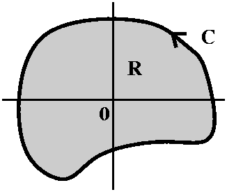 Let's look at ∫C[u(x,y)dx–v(x,y)dy] with p=u and q=–v. Then
qx–py is –vx–uy. But one
of the Cauchy-Riemann equations is uy=–vx, so
the integrand in the double integral over R is 0.
Let's look at ∫C[u(x,y)dx–v(x,y)dy] with p=u and q=–v. Then
qx–py is –vx–uy. But one
of the Cauchy-Riemann equations is uy=–vx, so
the integrand in the double integral over R is 0.
Let's look at ∫C[v(x,y)dx+u(x,y)dy] with p=v and q=u. Then
qx–py is ux–vy. The other
Cauchy-Riemann equation is ux=vy, so the
integrand in this use of Green's Theorem is 0 also.
Both the real and imaginary parts are 0, so the integral is 0. We're done.
A note about Goursat
The key hypothesis in Cauchy's Theorem is that u and v are
continuously differentiable and satisfy the Cauchy-Riemann equations
in the appropriate region. But Goursat, late in the 19th
century, showed that that if f´(z) exists, then the conclusion of
Cauchy's Theorem follows. The continuity of the derivative is
unnecessary. The proof is in the text, and is quite clever. I won't
give it here, because to my knowledge the techniques of the proof are
rarely used in most of complex analysis.
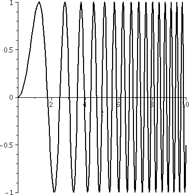
An example and exercise: Fresnel
This is problem 13 in section 2.3, and is a very neat direct
application of Cauchy's Theorem. The problem is to compoute
FresnelC=∫0∞sin(t2)dt
and
FresnelS=∫0∞cos(t2)dt,
the "Fresnel integrals" (more about them in a second). This is a
standard use of complex analysis. There are other methods of computing
this integral but this is the customary may.
It may be difficult to convince yourself that the integrals even exist
before we compute them. But look at the graph of sin(t2)
from 0 to 10. The alternating "bumps", getting narrower and narrower,
clearly (?) almost cancel each other out.
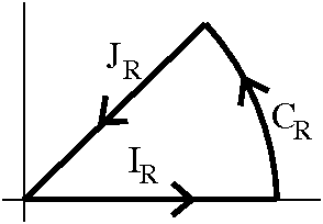 Let's compute the integral of f(z)=eiz2 around the
simple closed curve from 0 to R (R large, real, positive) then around
a circular arc to (1+i)R/sqrt(2), and then back to the origin. Since
f(z) is entire, the integral is 0 for any R. I'll call IR
the line segment along the real axis, CR the circular arc,
and JR the line segment "returning" to 0. Cuachy's Theorem
implies that
∫IR+CR+JRf(z) dz=0.
Let's compute the integral of f(z)=eiz2 around the
simple closed curve from 0 to R (R large, real, positive) then around
a circular arc to (1+i)R/sqrt(2), and then back to the origin. Since
f(z) is entire, the integral is 0 for any R. I'll call IR
the line segment along the real axis, CR the circular arc,
and JR the line segment "returning" to 0. Cuachy's Theorem
implies that
∫IR+CR+JRf(z) dz=0.
Getting rid of CR
This mostly should look familiar. We parameterize CR with
z=Reit so dz=Ri eitdt and
z2=R2e2it. Then the integral over
CR becomes
∫t=0t=Π/4eiR2e2itRi eitdt.
The modulus of this integral is bounded by
∫t=0t=Π/4eRe(iR2e2it)R dt.
What is the real part of iR2e2it? We're
considering i R2(cos(2t)+i sin(2t)). The real
part is –R2sin(2t).
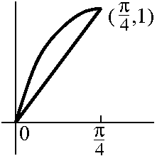 Notice that sin(2t) is increasing
and concave down on [0,Π/4], and therefore sin(2t)≥4t/Π on
that interval. Thus
–R2sin(2t)≤–R2(4t/Π). So the
modulus of the integral on CR is overestimated by
∫0Π/4Re–R2(4t/Π)dt
which can be computed exactly: it is
Re–R2(4t/Π) (–R2(4/Π))–1]0Π/4=(Π/{3R})(1–e–R2). This surely →0 as R→∞.
Notice that sin(2t) is increasing
and concave down on [0,Π/4], and therefore sin(2t)≥4t/Π on
that interval. Thus
–R2sin(2t)≤–R2(4t/Π). So the
modulus of the integral on CR is overestimated by
∫0Π/4Re–R2(4t/Π)dt
which can be computed exactly: it is
Re–R2(4t/Π) (–R2(4/Π))–1]0Π/4=(Π/{3R})(1–e–R2). This surely →0 as R→∞.
What happens to JR?
Here we have z={(1+i)/sqrt(2)}t, going from R to 0. So
dz={(1+i)/sqrt(2)}dt and
iz2=i(i)t2=–t2. Therefore
∫JReiz2dz=–{(1+i)/sqrt(2)}∫0Re–t2dt.
Now as R→∞ this integral converges to a well-known (if you
don't know, I will show it to you in a second!) VALUE. So
∫0Re–t2dt→
∫0∞e–t2dt=VALUE. The limit of
∫JReiz2dz is
–{(1+i)/sqrt(2)}VALUE as R→∞.
And the integral on IR
Here z=t, a real parameter. Then
eit2=cos(t2)+i sin(t2), and
therefore since the integral around
IR+CR+JR is always 0, we learn (since
the CR→0 and the JR integral approaches a
limit) that the IR integral approaches –(–{(1+i)/sqrt(2)}VALUE). But
∫JReiz2dz=
∫0Rcos(t2)dt+i∫0Rsin(t2)dt.
Therefore the limits exist, and
the value is FresnelC+iFresnelS.
so
FresnelC and FresnelS are both
equal to VALUE/sqrt(2).
What is this "VALUE"?
We'll be able to get this in another week of this course using complex
variable methods. But here is a quick way to compute it from calc 3
which you may have seen before. We compute twice the value of VALUE:
(∫0∞e–t2dt)2=∫0∞e–x2dx·∫0∞e–y2dy=∫0∞∫0∞e–x2e–y2dx dy
∫∫R2e–(x2+y2)dAx,y.
But this last double integral has circular symmetry in both the
integrand and the domain so conversion to polar coordinates may be
useful:
∫θ=0θ=2Π∫r=0r=∞e–r2r dr dθ=2Π{–(1/2)}e–r2]0∞=Π (yes, everything should
have limr→∞).
So VALUE=sqrt(Π)/2 and both
FresnelC and FresnelS are
Π/[2sqrt(2)].
The Fresnel
integral is used in many engineering and physics applications
(railroad tracks and diffraction!) and a related curve, the Cornu or Euler
spiral, is essentially the only plane curve with curvature
proportional to the length from a starting point (κ=s for those
who remember the letters and their meaning): a curve with a simple
geometric property but with a rather complicated algebraic
description.
Exams were returned. Here is information about
the grading of the exam.
| Monday,
March 1 | (Lecture #12) |
|---|
ADVERTISEMENT LEARN CAUCHY'S THEOREM. ADVERTISEMENT
Today we'll discover more about power series. We will see the reasons
that power series are computationally effective. The underlying
rationale is the amazing strength of GEOMETRIC
SERIES. The whole subject depends on
∑j=0∞arj=a/(1–r)
for |r|<1.
The explanations I give below were probably first understood and
explained by Weierstrass, an ancestor of the
course instructor.
I will discuss the following statements about series of the form
&sumj=0∞aj(z–z0)j,
where {aj} is a sequence of complex constants. Such a
series is said to be a power series centered at z0. Then:
- Each power series has a radius of convergence, R. R is one of
these numbers: [0,∞]. By this I mean:
- If R=0, then the series converges only when
z=z0. The series diverges for all other z's.
- If R=∞, then the series converges absolutely and
therefore converges for all complex numbers, z.
- If 0<R<∞, then the series converges absolutely and
therefore converges for all complex numbers, z, with
|z–z0|<R and the series diverges for all complex
numbers, z, with |z–z0|>R.
- Suppose R≠0. Then the sum of the series, inside the radius of
convergence, is a continuous function.
- Suppose R≠0. Then the sum of the series, inside the radius of
convergence, is a complex differentiable function whose derivative is
the sum of the series
&sumj=0∞j aj(z–z0)j–1
which has the same radius of convergence.
We know by our experience both in calc 2 and in this course that in
many specific examples, we can use methods like the Ratio and Root
Tests and that the "output" from these tests is a conclusion like the
first statement. And we've seen examples with R=0 and R=∞ and
any R in between. What this statement declares is that any
power series behaves qualitatively like the examples we've seen. The
methods to get R are neat, but all the series must behave this
way. There's never a square of convergence or maybe convergence in two
disconnected "lumps". This simple behavior is not true for
other series, but it is true for power series: easy to understand.
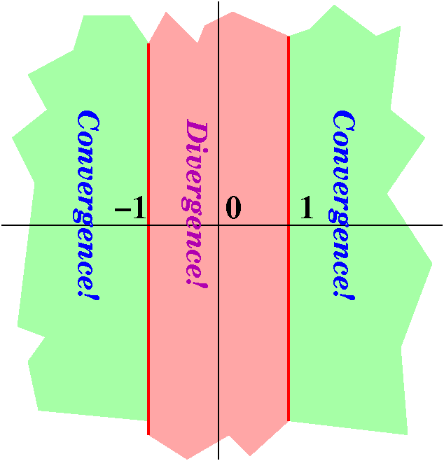
Here: consider the ugly and unlikely series
∑j=1∞(e(1–[Re(z)]2))j. This is a geometric series with a weird
ratio. It converges if e(1–[Re(z)]2) is less
than 1. Let's see: that means the input to exp should be negative:
1–[Re(z)]2<0 or 1<[Re(z)]2. So the series
converges in the union of two halfplanes,
{Re(z)<–1}∪{Re(z)>+1} and diverges for
{–1≤Re(z)≤1}. This example is not interesting to me but it does
show that the first statement does have content.
The second statement declares that the sum of a power series, inside
its radius of convergence (a domain, a connected open set), is
continuous. Anyone with experience with Fourier series knows that a
similar statement about Fourier series is false. Fourier series
can converge to terrible functions, with jumps and loathsome (!!)
wiggles. Well, not loathsome, but certainly strange. This is the
useful but complicated nature of Fourier series. But power series are
so nice.
The third statement has a whole collection of consequences. For
example, it can be applied repeatedly to show that the series can be
differentiated any number of times. Then, by evaluation at
z0, the coefficients of the series can be identified with
the coefficients of a Taylor series centered at
z0. Therefore any power series with R≠0 must be a Taylor
series, and any function which is the sum of a power series centered
at z0 has exactly one such series, so any (legitimate!) way you get a power series for a function
gives the correct answer. I'll go over this in detail.
In what follows I'll only look at the case z0=0 because
this is less writing. There will be times in this course and in
applications that we can't always take z0=0: it just won't
be natural. But right now, I opt for this easier alternative.
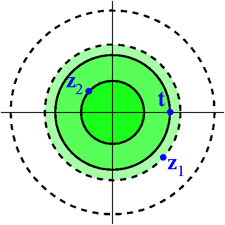 Everything starts with the following statement:
Convergence propagates inward
If
∑j=0∞ajzj
converges for z=z1≠0, and if
|z2|<|z1|, then the series converges for z2.
This is the easiest claim, and the way to understand why it is correct
is a prototype for all of the others. So we know that
∑j=0∞ajz1j
converges. Since the series converges, the terms →0. (The
converse isn't true [Alternating Harmonic Series!] but the assertion
this way is true.) This means that the individual terms all are a
collection of numbers inside some (finite!) disc centered at 0. So
there is M>0 so that |ajz1j|<M. Now take some positive real number t with
|z2|<t<|z1|. Look at the picture, please:
there certainly is a lot of room to select such t. Then t=(t/|z1|)|z1|. The
number t/|z1| (think of it as r) is a positive number less
than 1. So a geometric series with ratio t/|z1| must
converge. Therefore the series
∑j=0∞M(t/|z1|)j
converges. But
|aj|tj=|aj|(t/|z1|)j|z1|j≤Mrj.
And further, |ajz2j|<|ajtj|<Mrj. The
modulus of each term of the power series at z2 is less than
the corresponding term of a convergent positive geometric
series. Therefore the series converges absolutely at
z2, and thus it converges: convergence propagates inward!
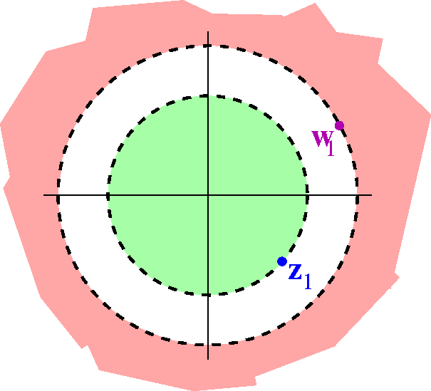 Showing why the first statement is true
Now let's look at the whole situation. Suppose the series converges at
z1 and diverges (doesn't converge) at w1. Well,
certainly |z1|≤|w1| or else we'd be
contradicting the propagation of convergence. But now I know that the
series converges for all z's with |z|<|z1| and I also
know that the series diverges for all w's with
|w|>|w1|. Divergence propagates outward or else
we'd have a contradiction. So "color" the plane into convergent and
divergent points. The only way we don't contradict the facts we now
know is for these "colors" to meet up at one circle, a circle of
radius R and that convergence occurs inside the circle and divergence
outside the circle. If there's no such circle, we're in
trouble. Notice, please, that I am not discussing the coloring of the
circle itself -- I am not concerned with that here.
 How the sum of the series behaves
Now let me move ahead and discuss what happens to the sum
inside the radius of convergence, R. Here I will assume that R
is not 0 because I want to compare values of the sum at two
different points. For |z|<R, let me define f(z) to be the value of
∑j=0∞ajzj. This
is, remember, the limit of the partial sums: I am still not adding up
infinitely many numbers! Let me again take some t which is between 0
and |z1| where the series converges at z1. I
will take any two complex numbers z2 and z3 with
|z2| and |z3| both ≤t, and I will try to
convince you that if |z2–z3| is small, then I
can make |f(z2)–f(z3)| as small as I want.
Well,
f(z)=∑j=0∞ajzj=∑j=0Najzj+∑j=N+1∞ajzj.
I have split the sum up into a finite sum and an "infinite
tail". Remember that our z's of interest have modulus at most t. And
also remember that |∑j=N+1∞ajtj|≤∑j=N+1∞Mrj.
This second infinite series is a geometric series, and its sum is
MrN+1/(1–r) where r is a number less than 1. I can make
this very small by selecting N large.
Showing why the second statement is true
So I want to "control" |f(z2)–f(z3)|. Let's say
I want this to be less than some really small positive number Q. I am
going to outline a method which can actually be used numerically in
applications. Well, first select N so that the tail will be less than
Q/3. Then, having done that, look at this description of the
difference:
f(z2)–f(z3)=∑j=0∞ajz2j–∑j=0∞ajz3j=(∑j=0Najz2j+∑j=N+1∞ajz2j)–(∑j=0Najz3j+∑j=N+1∞ajz3j).
So I have two polynomial pieces and two infinite tails. If I drop the
two infinite tails, the errors I'll make in modulus are at most
2Q/3. What about the other pieces? Well, we have
∑j=0Najz2j–∑j=0Najz3j.
These are finite sums and I'm not afraid of finite sums. In
fact, this is just ∑j=0Naj(z2j–z3j). Can I make this small? Now we're discussing whether
polynomials are continuous. Actually, I won't go through the
details (they can be found in any of our hugely thick calc 1
textbooks) but by making |z2–z3| very small (and
also both with modulus at most t), I can make the difference of the
modulus of the values of a fixed polynomial at z2 and
z3 small. I can make the difference less than Q/3, in fact.
If you give me a specific power series, these estimates can be carried
out computationally. You may not like them, but the process is quite
effective.
The differentiated series
Now, finally, I want to address the third claim, about
derivatives. This is more complicated. The computations can also be
carried out numerically, but definitely the effort is more
elaborate. Suppose that the series for f(z) converges for
z1 and, as before, t is a real positive number with
t<|z1|. So I know that
∑j=0∞ajtj
converges because we compared it to
∑j=0∞Mrj. But, wait: the
series ∑j=0∞jMrj–1 also
converges absolutely! I can use the Ratio Test, for example, and since
r<1 and limj→∞(j+1)/j=1, the extra j in front
doesn't matter. Since
∑j=0∞jMrj–1 converges
absolutely, we know that
∑j=0∞j ajtj–1
converges absolutely by comparison. And then we know that
∑j=0∞j ajz2j–1
converges absolutely for any z2 with
|z2|≤t. Therefore (again, again, again!) this "termwise
differentiated" series converges. Call its sum g(z). This logic, if
examined closely, shows that the radius of convergence of the series
∑j=0∞j ajzj–1
is the same as that of the original series.
Are we done? No, we are not done!!!
The logic is quite involved. We have a power series
∑j=0∞ajzj which
converges to f(z) when |z|<R. We have a power series
∑j=0∞j ajzj–1
which converges to g(z) when |z|<R. Why should f´(z)
exist, and, if it does, why should to be equal to g(z)? This is
exactly what goes wrong with things like Fourier series. You
write stuff that looks good, but then if you try to verify what you
really want to be true (or, better yet, compute all these things
numerically) then it doesn't work.. This sort of experience
which led to a great deal of confusion historically.
A detailed verification that f´ exists and equals g is in the
textbook. I'll try to give some reasons to expect that this is
correct. Almost every complex analysis book has slightly different
reasoning here, because the sums and the related algebra are
intricate. The slickest verification I know is in a book, Complex
Analysis by Kunihiko Kodaira (in the math library, in the QA331
section). I don't want to present it because ... it is just too
good. You read it and can't see any difficulties. So I'll be much more
ordinary.
Let's start with monomials, zj, and consider z's with
|z|<t and t<|z1| so the series for f(z1)
converges. Differentiation means that we need to compare
[(z+h)j–zj]/h with jzj–1 for h's with
|h| very small. In fact, let me choose make h so that
|h|≤SMALL=|z1–t|/100. I don't think 100
is needed, but I don't much care -- if I were implementing this
numerically, I would need to go over everything really carefully, but
here I just want to give a poetic (!) impression. If you don't like
algebra or binomial coefficients, go to sleep for 5 minutes because
the reasoning will be very dense.
(z+h)j=∑k=0jCkjzj–khk
where Ckj are binomial
coefficients. This is the simplest finite version of the Binomial
Theorem which has been discovered and rediscovered in culture
after culture (China, Greece, India, Persia, and, much later,
France!). The beginning of the sum is interesting here:
∑k=0jCkjzj–khk=zn+nzn–1h+h2JUNK.
If we were only interested in the differentiation of zj (as
in calc 1) we can stop here because this tells me that
{[(z+h)j–zj]/h}–nzj–1 is
hJUNK and that as h→0 things
→0. The trouble here is that we're going to be adding up linear
combinations of these monomials (multipling them by the coefficients
aj) and then taking limits (we are considering
infinite series!) and we need to worry about how big infinitely
many JUNK terms are! This is not
so easy, not only because we have infinitely many terms, but also
because the binomial coefficients can get really
big.
So, in more detail,
{[(z+h)j–zj]/h}–nzj–1 is
∑k=2jCkjzj–khk–1.
The k–1 in the exponent occurs because I'm dividing by h in the
difference quotient for zj. The lower bound on the sum is
k=2 because the 0 and 1 terms drop out (because of –zj,
division by h, and –nzj–1).
I want to estimate the modulus of this, which is |∑k=2jCkjzj–khk–1|. Of course I'll use the Δ≤ to overestimate
and get
∑k=2jCkj|z|j–k|h|k–1.
This is almost like the original Binomial Theorem. I really will need
|h| "outside" in order to squeeze this small, so I rewrite (150 years
of irritation!) the sum as
|h|∑k=2jCkj|z|j–k|h|k–2.
Now wait: for the |h|'s inside the sum I will do a different
overestimate: |h|≤SMALL. Then
the overestimated sum becomes
∑k=2jCkj|z|j–kSMALLk–2.
But
A–2Ak=Ak–2 so
∑k=2jCkj|z|j–kSMALLk–2=∑k=2jCkj|z|j–kSMALL–2SMALLk=SMALL–2∑k=2jCkj|z|j–kSMALLk. We can make this bigger
(overestimate it) by taking the sum, which starts at k=2 and
changing this lower bound to k=0. So here is something bigger:
∑k=0jCkj|z|j–kSMALLk. The Binomial Theorem
tells me that I can write this more compactly as (|z|+SMALL)j. This is less than, in
turn,
(t+SMALL)j.
Sort of showing why the third statement is true
There are lots of details, which are written in your textbook. The
whole thing seems like a really big cheat: we used the Binomial
Theorem to unpack a power of a sum (more or less at z+h), and then we
manipulate things and repack a sum into a different power (more or
less at z+SMALL).
Here's another thing: I can now think of t+SMALL as a new "t", let me call it
t1, which is just as valid as t. And I can wrap up the whole
series, just as in the very first part of this discussion, by
overestimating it by |h|SMALL–2∑j=0∞|aj|(t1)j.
Now the only thing "changing" is |h| as h→0, so we get a
verification that the derivative of the infinite series is the
infinite series of the differentiated terms because the error between
the difference quotient for whole series and the infinite series for
the derivative candidate is →0.
|
We needed the special forms of the geometric series and the Binomial
Theorem. The reasoning is very specific. I will show you some common
examples using Fourier series where things just don't work
because these results are not available.
I needed to prepare very carefully for this lecture, unlike
almost all the others in the course! This is certainly the most
technical reasoning in the course, and I will not again need to refer
to these estimates or these methods. But you will see why the logic of
the statements we discussed today are a very important part of complex
analysis.
| Wednesday,
February 24 | (Lecture #11) |
|---|
What I did last time was remarkably subtle
stuff. Experience teaching exactly that material a
number of times on both the graduate and undergraduate levels has
taught me that understanding what I would hope was "simple"
computations instead turns out to be, for some people, rather an
upsetting collection of computations and ideas. I hope you will learn
from that class.
Today, I want to continue the schizophrenia (?) of the subject, and at
least initially concentrate on a specific example of an analytic
(indeed, entire!) funtion: sine.
What should sin(z) be? I'm not even asking whether there should be a
function called sin(z), because if there is not, then we should
abandon our attempts to do calculus with complex numbers. I'll outline
one approach which is perhaps somewhat idiosyncratic (the noun: "a
mental constitution, view or feeling, or mode of behaviour, peculiar
to a person."). It turns out that there's only one answer, but many
ways to "guess" the answer.
Well, sin(z)=sin(x+i y) should
be sin(x)cos(i y)+cos(x)sin(i y). This
doesn't seem to help too much because now I'm faced with
cos(i y) and sin(i y). I could guess at thses knowledgeably
just as I did earlier in the course with ei t and
learning about the differential equations they satisfy along with the
initial conditions. Let me try another approach, just for fun.
What should cos(i y) be? Well, from calc 2 I know about Taylor
series and about the remainder term and about ... well, lots of
things. In particular, one of the simplest applications is that the
infinite series
1–t2/2!+t4/4!–t6/6!+... converges for
all t, and that the sum of this series is cos(t). well, we know it
converges now for all complex t because we could apply, again, the
Ratio Test, learn that the series converges absolutely for all complex
t, and therefore must converge for all complex t. But if we insert
i y for t, and take powers then we seem to get
1+y2/2!+y4/4!+y6/6!+... and maybe we
recognize that these are the even powers of the exponential
function. So this is {ey+e–y}/2. And this has a
name: it is called cosh(y), the hyperbolic cosine of
y. The word "cosh" has a non-technical meaning: "A weighted weapon
similar to a blackjack."
Similarly, I can take sin(i y) and feed i y into the series
for sine:
t–t3/3!+t5/5!–t7/7!+.... The
convergence discussion for this series is entirely similar to what
happens with cosine, so when we plug in i y the result is i(y+y3/3!+y5/5!+y7/7!+...). What's inside these parentheses are the odd powers
of the exponential function, and therefore we can get them by
subtracting e–y from ey and dividing by
2. And don't forget the i. The sum of the series (without the i!) is
called sinh(y) (hyperbolic sine, pronounced like the English
word "cinch" which means "Something easy to accomplish.").
Let me steal the following table from the last time I taught Math 421,
Advanced Calculus for Engineers:
| What every child should know about
trig and hyperbolic functions ... |
|---|
TRIG
onometric |
cosine | cos(0)=1
cos´(0)=0 |
y´´=–y | cos(t)=([eit+e–it]/2)
| It wiggles between –1 and 1
always | 
|
|---|
| sine | sin(0)=0
sin´(0)=1 |
y´´=–y | sin(t)=([eit–e–it]/2i) |
It wiggles between –1 and 1 always | 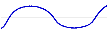 |
HYPER
bolic |
cosh | cosh(0)=1
cosh´(0)=0 |
y´´=y | cosh(t)=([et+e–t]/2)
| It gets big both ways
both sides are + |
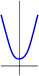 |
|---|
| sinh | sinh(0)=0
sinh´(0)=1 |
y´´=y | sinh(t)=([et–e–t]/2) |
It gets big both ways
+ on the right; – on the left |
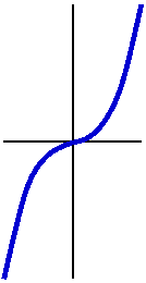 |
Let me add further that just as the parametric curve (cos(t),sin(t))
describes the unit circle, the pair of functions (cosh(t),sinh(t))
describes a point on the curve x2–y2=1. Just
plug in: (et+e–t}/2)2–({et–e–t}/2)2=(1/4)(e2t+2–e–2t–{e2t–2–e–2t)=4/4=1.
The picture below summarizes this situation (and no, I don't want to
go into details!).
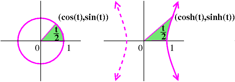
Back to (complex) sine
We know that sin(z)=sin(x)cosh(y)+i sinh(y)cos(x).
We checked by direct computation that
sin(x)cosh(y) and sinh(y)cos(x) are harmonic: Δ[sin(x)cosh(y)]=0
and Δ[ sinh(y)cos(x)]=0. On the way we also got evidence
that the Cauchy-Riemann equations are satisfied, so that
sinh(y)cos(x) is a conjugate harmonic function for sin(x)cosh(y).
So this is an analytic function, the only version of sine that people
want.
The image of the real axis is the interval [–1,1] (just the
usual values of sin(x) since sinh(0)=0) and the image of the imaginary
axis is (x=0!) all of the imaginary axis (i sinh(y)).
When is sin(z)=0? Then the imaginary part=0 implies that either
sinh(y)=0 or cos(x)=0. If sinh(y)=0, then y=0. If cos(x)=0 then x is
Π multiplied by (odd integer)/2. But then sin(x) wouldn't be 0
and cosh(y) is never 0. So therefore we must have y=0 and
x=2Π(an integer). Therefore sin(z) has the same roots as the
usual sine function.
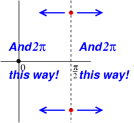
But could sin(z)=2? Let's see: again, sinh(y)cos(x) would have to be
0. sinh(y) could be 0 but then the real part wouldn't get big
enough. So cos(x) should be 0. sin(x) will be ±1. Since cosh is
always positive, let's make sin(x)=1, say with x=Π/2. Then select y
so that cosh(y)=2. Can we do this? Well, we get a quadratic equation
in ey, and the result is y=ln(2±sqrt(3)). So
sin[(Π/2)+i ln(2±sqrt(3))] is 2. Is this distressing? Are
there other solutions? Well, yes, all separated by integer multiples
of 2Π. Notice, please, that ln(2+sqrt(3)) is –ln(2–sqrt(3)), so the
solutions we just found are shown to the right. Only two of a
doubly infinite family of the solutions are shown!
The mapping properties of sine are new. Let me reproduce figure 1.25
of the textbook:
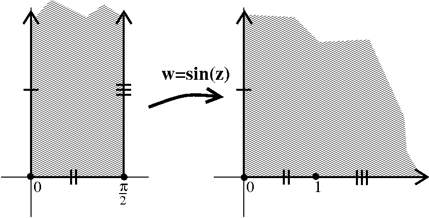
When x=0, we get sin(0+i y)=0+i sinh(y), so the image of the
positive imaginary axis is the positive imaginary axis. For y=0 and x
between 0 and Π/2, the image is the interval [0,1] on the real
axis. But when x=Π/2, then we get
sin(Π/2+i y)=sin(Π/2)cosh(y)+i sinh(y)cos(Π/2)=cosh(y).
As y goes from 0 to ∞, the image point moves from 1 to ∞
on the positive real axis. Then some more thought shows that
the image of the half strip is a quarter plane.
 What happens to horizontal and vertical paths under the sine mapping?
Here I didn't have time in class (but the computations are in the book
(section 1.5). The horizontal line segments get changed to the first
quadrant part of ellipses. As the horizontal line segments move down
to the real interval [0,Π/2], the image ellipses collapse to the
interval [0,1]. The vertical half lines all turn into halves of
hyperbolic arcs. As we will see later due to very general theorems,
since the blue and green curves generally intersect orthogonally,
their images are also orthogonal. In general, angles are
preserved. But a strange thing happens at Π/2. There sin(Π/2)=1
and sin´(Π/2)=cos(Π/2)=0. Locally Taylor's Theorem is still
valid, and for z near Π/2,
sin(z)=sin(Π/2)+sin´(Π/2)(z–Π/2)+[sin´´(Π/2)/2](z–Π/2)2+H.O.T.
(that "H.O.T." is, of course, "higher order terms"). Then
locally,
sin(z)=1+(–1/2)(z–Π/2)2+H.O.T.. Squaring doubles
angles locally, so the right angle becomes a straight angle. This is
the only point in the picture where angles are not preserved
under the sine mapping.
What happens to horizontal and vertical paths under the sine mapping?
Here I didn't have time in class (but the computations are in the book
(section 1.5). The horizontal line segments get changed to the first
quadrant part of ellipses. As the horizontal line segments move down
to the real interval [0,Π/2], the image ellipses collapse to the
interval [0,1]. The vertical half lines all turn into halves of
hyperbolic arcs. As we will see later due to very general theorems,
since the blue and green curves generally intersect orthogonally,
their images are also orthogonal. In general, angles are
preserved. But a strange thing happens at Π/2. There sin(Π/2)=1
and sin´(Π/2)=cos(Π/2)=0. Locally Taylor's Theorem is still
valid, and for z near Π/2,
sin(z)=sin(Π/2)+sin´(Π/2)(z–Π/2)+[sin´´(Π/2)/2](z–Π/2)2+H.O.T.
(that "H.O.T." is, of course, "higher order terms"). Then
locally,
sin(z)=1+(–1/2)(z–Π/2)2+H.O.T.. Squaring doubles
angles locally, so the right angle becomes a straight angle. This is
the only point in the picture where angles are not preserved
under the sine mapping.
We checked by direct computation that sin(–z)=–sin(z) and that
sin(z)=sin(z). Then (look at
conjugation followed by –) the half strip defined by
–Π/2<x<Π/2 and $y>0 gets mapped by conjugation and
minusing into the second quadrant. The result is this:
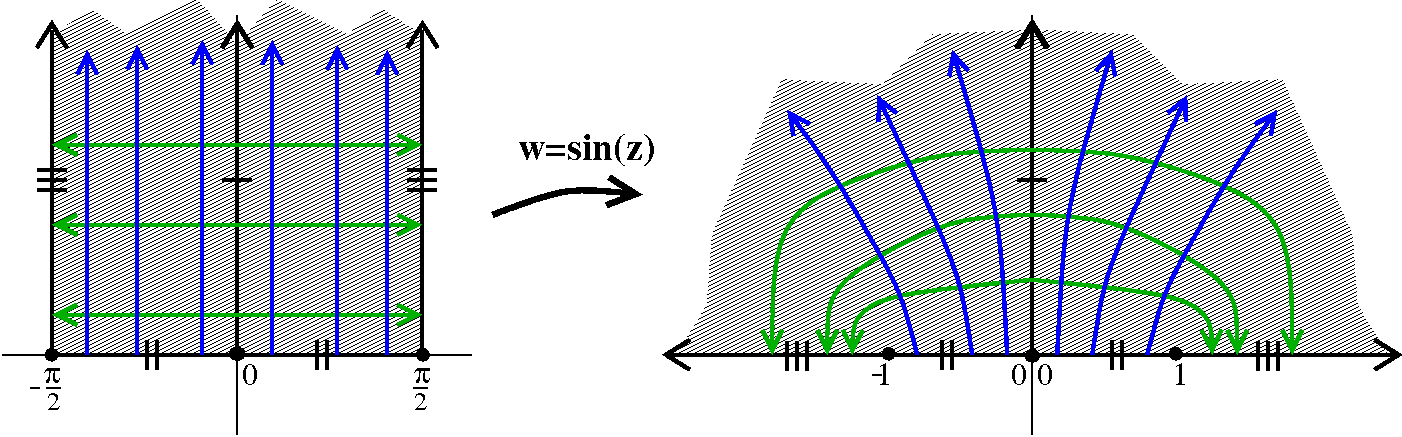
Can we get the lower halfplane? Yes, since
sin(–z)=–sin(z), the lower half strip gets mapped to the lower
halfplane. Every vertical strip which is 2Π wide gets mapped
ONTO all of C!
Other functions
Cos(z) and sinh(z) and cosh(z) are all like this. They are new and can
be understood. The real problems occur with something like
arcsin. We'll see if there is enough time in the course to deal with
that.
| Monday,
February 22 | (Lecture #10) |
|---|
I'll review the definitions of analytic function. A trick question:
where is |z|2 analytic? Since it is complex differentiable
at only 1 point (the origin) there is no open set in which it
is complex differentiable and therefore it is not analytic in any open
set. A domain is a connected open set, and an entire
function is analytic in all of C.
I'd like this statement to be correct:
If f´(z)=0 always, then f is
constant.
But it is not. Here is an example: if I have, say, a function
which is defined in two disconnected blobs, and is 56 in one of them
and –7i in the other. The missing ingredient is connected. So:
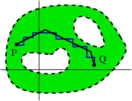 Theorem If f is analytic in a domain and if f´(z)=0
always, then f is constant.
Theorem If f is analytic in a domain and if f´(z)=0
always, then f is constant.
A proof is that if f´(z)=0 then ux=0 and
uy=0 and vx=0 and vy=0 using the
Cauchy-Riemann equations. Then in a connected open set, I can connect
two points by a piecewise linear path. In fact, if you look closely, I
can modify this to a piecewise linear path whose pieces are parallel
either to the x- or y-axes. But along either of these, u and v cannot
change (apply FTC to the correct derivative -- on a horizontal sement,
for example, the difference in u at the endpoints is the definite
integral of ux along that path, so the difference is
0). Then u and v cannot change along the path, so its value at a
random two points must be the same.
There are simple consequences of the Cauchy-Riemann equations which
are quite neat. So I can tell you that there are not very
many analytic functions which are always real. In fact, if v(x,y)=0
always, then f(z) is constant. (In a domain, darn it!). Because
then vx and vy are both always 0, and
(Cauchy-Riemann equations again) we deduce that ux and
uy are always 0, so we are reduced to the previous
assertion.
Consider z2, which is certainly entire. Its real part is
x2–y2. Is there an analytic function whose real
part is just, say, x3? The answer is no. Let's see why. If
u=x3, then ux=3x2 and
uy=0. Then I know (Cauchy-Riemann equations!) that
vy=3x2 and vx=0. But vyx
must be the same as vxy, and since 6x is rarely equal to 0,
this is impossible!
It is time to make a few more definitions. A real-valued function
(sufficiently differentiable!) h(x,y) is called harmonic if
Δh=0. By Δ I mean the following silly thing:
∂2/∂x2+∂2/∂y2.
This is called the Laplace operator and is very important in
theory and in applications (it is the only rotationally symmetric pure
second order operator).
Theorem If f(z)=u(x,y)+i v(x,y) with u and v both twice
differentiable, then both u and v are harmonic functions.
Let me compute: ∂u/∂x must be ∂v/∂y (CR!). So
∂2u/∂x2 is
∂2v/∂y∂x. But also ∂u/∂y is
–∂v/∂x, so ∂2u/∂2y is
–∂2v/∂x∂y. But mixed partials should be
equal (in this courses, all of our functions will be very
differentiable so we won't need to worry about bad examples
here). Therefore the sum of ∂2u/∂x2
and ∂2u/∂2y will be 0.
Now v is the real part of the analytic function –i f
(switches u and v and puts a + sign on v) so since v is the real part
of an analytic function, it also is harmonic.
Examples include x2–y2 and excos(y)
since these are the real parts of an analytic function. But I can't
just push these together and hope that the result is analytic, because
(x2–y2)+i(excos(y)) is not
analytic. The real and imaginary parts of an analytic function must be
specially linked.
Definition Suppose u and v are harmonic functions. Then v is a
harmonic conjugate of u if u+i v is analytic.
So the problem I then posed students was: given a harmonic function
h(x,y), how can we "create" a harmonic conjugate, g. Well, after some
thought, people remarked that if the CR equations were to be true,
then the hypothetical function g(x,y) would need to satisfy:
∂g/∂x=–∂h/∂y; ∂g/∂y=∂h/∂x.
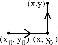 These are just the CR equations "backwards". Since I am supposed to
know how g "changes" (gx and gy) I should be
able to reconstruct g from its value at 1 point. For example, suppose
I knew g(x0,y0) and wanted g(x,y). I could
integrate gx from (x0,y0) to (x,y0) and then integrate
gy for (x,y0) to (x,y). So I get the following intricate
recipe (replacing the partial derivatives by the known partial
derivatives of h):
These are just the CR equations "backwards". Since I am supposed to
know how g "changes" (gx and gy) I should be
able to reconstruct g from its value at 1 point. For example, suppose
I knew g(x0,y0) and wanted g(x,y). I could
integrate gx from (x0,y0) to (x,y0) and then integrate
gy for (x,y0) to (x,y). So I get the following intricate
recipe (replacing the partial derivatives by the known partial
derivatives of h):
g(x,y)=g(x0,y0)+∫x0x–∂h/∂y(t,y0) dt+∫y0y∂h/∂x(x,s) ds
I used t for the parameter along the horizontal line and s for the
parameter along the vertical line. I would like to verify that the
function g I created has the correct partial derivatives. Well, the
formula I just wrote only has y appearing once and there as an
upper parameter of a definite integral. Therefore ∂g/∂y is
∂h/∂x(x,y) using FTC on the second integral (the first
integral has no y in it so its derivative is 0 with respect to
y). I would like to check the x derivative, but maybe I could just
write a different integral, like this:

g(x,y)=g(x0,y0)+∫y0y∂h/∂x(x0,s) ds+∫x0x–∂h/∂y(t,y) ds
Now, using this formula, there is only one appearance of x, and
I can compute using FTC again to get
∂g/∂x=–∂h/∂y.
So I verified that the partial derivatives are what they should be and
I have "created" a harmonic conjugate. The only difficulty is that I
used two different formulas for the same quantity, g(x,y), and
why should these formulas give the same result?
They give the same result if the integral around the two paths is the
same. Wait: this is the same thing as asking that the integral all
the way around the (correctly oriented!) edge of the rectangle is
0. Let me subtract off the g(x0,y0) from both of the formulas, and
reverse the orientation of the top & left path. Then I want to compute
the line integral:
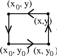 ∫C(–∂h/∂y)dx+(∂h/∂x)dy
where C is the boundary indicated of the rectangle. Maybe we should
use Green's Theorem with P(x,y)=–∂h/∂y and
Q(x,y)=∂h/∂x. The integrand in the double integral side of
Green's Theorem is ∂Q/∂x–∂P/∂y.
If Q(x,y)=∂h/∂x, then ∂Q/∂x=∂2h/∂2x.
If P(x,y)=–∂h/∂y, then –∂P/∂y=–(–∂2h/∂2y).
The sum of the right-hand sides is Δh which is 0 since h is
harmonic so the double integral is actually integrating 0, and the
line integral side of Green's Theorem is 0 also. Therefore the two
integrals are computing the same thing, and we are correct.
A specific example
So I tried to consider h(x,y)=ln(x2+y2). I first claimed
this was harmonic and verified it:
hx=–2x/(x2+y2).
hy=–2y/(x2+y2).
Now the second derivatives:
hxx=[–2(x2+y2)–2x(–2x)]/(x2+y2)2=(2x2–2y2)/(x2+y2)2.
hyy=[–2(x2+y2)–2y(–2y)]/(x2+y2)2=(2y2–2x2)/(x2+y2)2.
It is almost amazing that
Δh=∂2h/∂x2+∂2h/∂x2=0 since the tops
cancel.
How to "create" (attempt to create) a harmonic conjugate
I switch x and y derivatives and insert a minus sign. The line
integral I should consider is (–∂h/∂y)dx+(∂h/∂x)dy
which is
2y/(x2+y2)dx–2x/(x2+y2)dy.
I will assume for simplicity that the harmonic conjugate I am
attempting to create for this h(x,y) has value equal to 0 at (–1,–1),
and I will try to compute (actually compute, actually get a
value!) for h(1,1). 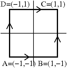 Well, if you consider the accompanying diagram, one way
I could get from (–1,–1) to (1,1) is by way of the piecewise linear
path ABC. So this integral is
Well, if you consider the accompanying diagram, one way
I could get from (–1,–1) to (1,1) is by way of the piecewise linear
path ABC. So this integral is
∫x=–1x=1–2/(x2+1)dx+∫y=–1y=1–2/(1+y2)dy.
This is because y=–1 on AB and dy=0, and, on BC, x=1 and dx=0. I can
compute these integrals. They are both arctan integrals, and the value
is –2Π.
I also could get from (–1,–1) to (1,1) is by way of the piecewise linear
path ADC. So this integral is
∫y=–1y=12/(1+y2)dy+∫x=–1x=12/(x2+1)dx.
This is because x=–1 on AD and dx=0, and, on DC, y=1 and dy=0. I can
compute these integrals. They are both arctan integrals, and the value
is 2Π.
These are supposed to be equal! What is the problem?
People thought about this, and several people volunteered that Green's
Theorem could not be applied with the specific second example I
was trying since ln(x2+y2) was not even defined
at (0,0) which is inside the square. Of course, that's the catch -- it
is easy to be deceived by formulas. I wrote precisely what I had
actually done:
TheoremSuppose h(x,y) is a harmonic function defined in all of
a disc (no holes!!!). Then h(x,y) has a harmonic conjugate
g(x,y) defined in that disc, g(x,y) is harmonic in that disc, and
h(x,y)Ii g(x,y) is analytic in all of that disc.
Example The function ln(x2+y2) is
harmonic in all of C except for 0. On that domain (it is
a connected open set, even though it has a "hole") the function
ln(x2+y2) has no harmonic conjugate.
This function is the real part of (1/2)log(z).
These are not obvious computations and not
obvious ideas. They took a great deal of time to develop.
As a final example, I pulled the function
x3–3xy2 out of a hat (must have been a
remarkable hat!). I verified that it was harmonic, and then just
guessed (hah!) at a harmonic conjugate:
3x2y–y3. Of course, I didn't guess. These
functions are the real and imaginary parts of the entire function
z3.
| Friday,
February 19 | (Lecture #9) |
|---|
SNOW DAY MAKE UP!!!
We stated this result last time.
Theorem Suppose u(x,y) and v(x,y) have continuous first partial
derivatives. Then limΔz→0(u(x+Δx,y+Δy)+i v(x+Δx,y+Δy))–(u(x,y)+i v(x,y))/Δz exists exactly
when (o.k., "if and only if") ux=vy and
uy=–vx.
We showed that if f is complex differentiable, then the
Cauchy-Riemann equations must be true. We actually saw that the
derivative, f´(z), is equal to both
(∂u/∂x)+i(∂v/∂x) and
(∂v/∂y) i(∂u/∂x).
Why is the converse assertion in the theorem true (reversing the logic
if...then)? Remember the following which is stated in
calc 3 but rarely verified, even though it only needs the Mean Value
Theorem of calc 1. If Q(x,y) has first partial derivatives which are
continuous, then
Q(x+Δx,y+Δy)=Q(x,y)+{∂Q/∂x}Δx+{∂Q/∂y}Δy+H.O.T..
The H.O.T. stands for "higher order terms" and stands
for "stuff" that →0 faster than any first order term in
Δx and Δy. For example,
limΔx→0H.O.T./Δx=0 and
limsqrt((Δx)2+(Δy)2)→0 H.O.T./sqrt((Δx)2+(Δy)2)=0. Now I'll use this applied to both the real and
imaginary parts of f.
f(z+Δz)=u(x+Δx,y+Δy)+i v(x+Δx,y+Δy)=
u(x,y)+{∂u/∂x}Δx+{∂u/∂y}Δy+H.O.T.1+i(v(x,y)+{∂v/∂x}Δx+{∂v/∂y}Δy+H.O.T.2)
This is very complicated but let me rethink a bit. First, I will
combine the two H.O.T.'s because the distinction between
them won't matter. Second, if I am assuming the Cauchy-Riemann
equations, then I could call {∂u/∂x}={∂v/∂y} by
one name, let's say A, and I could call
{∂u/∂y}=–{∂v/∂x} by another name, let's say –B (so
{∂v/∂x} is B, of course!). Then the material above becomes
this:
u(x,y)+AΔx–BΔy+i(v(x,y)+BΔx+AΔy)+H.O.T.
But let me recognize a bit more, if I realize that
(A+iB)Δz=(A+iB)(Δx+iΔy)=(AΔx–BΔy)+
(AΔy+BΔx) then the
preceding becomes
u(x,y)+i v(x,y)+(A+i B)(Δx+iΔy)+H.O.T.
Finally, rewrite in terms of z's and f's:
f(z+Δz)=f(z)+(A+i B)Δz+H.O.T.
This means that the quotient {f(z+Δz)–f(z)}/Δz is
A+i B+{H.O.T./Δz}. As Δz→0, the
last term also →0 because the top is "higher order". So the limit
exists and is A+i B. We have verified the claim above:
only the Cauchy-Riemann equations are needed to insure complex
differentiability.
Since the definition of complex differentiability is exactly like real
differentiability, I bet that the sum, product, quotient, composition,
etc. of complex differentiable functions is complex differentiable,
and that the derivatives obey the same algorithms as in "real"
calculus.
Complex differentiability turns out not to be exactly the correct
concept. For example, we saw that |z|2 is complex
differentiable, but only at z=0. That turns out to be a peculiarity,
and we need a bit more information. The key definition is the
following:
Key definition
Suppose U is a connected open set (a domain). Then a function f
defined on U is said to be complex analytic or
holomorphic if f is complex differentiable at all points of
U. We will also assume (this turns out to be logically not needed!)
that f´ is continuous. So a holomorphic function is one which is
defined and has a continuous complex derivative in a connected open
set. These are the functions discussed in this course.
I want to show you that already I know lots of things, so I will
compute infinitely many line integrals. First, though, some examples.
∫|z|=1x dz
Sometimes people omit the direction of a closed curve over which a
line integral is to be computed. In that case, almost always what's
meant is the counterclockwise orientation, so the "inside" is a
bounded region. What can I do here? I know that dz=dx+i dy, so we
need to compute ∫|z|=1x dx+i x dy. This
is ideal for applying Green's Theorem with P=x and Q=i x. Then
∂Q/∂x=i and ∂P/∂y=0, so we need to compute the
double integral of i over the inside of the unit circle. This is i
multiplied by the area, so it is Πi. You can also, if you wish,
compute this with a parameterization, etc.
∫|z|=1(1/z) dz
Maybe this is more interesting. Perhaps I would like to apply Green's
Theorem again. BUT 1/z is not
continuous everywhere inside the contour of integration. Hey: it isn't
defined at z=0! For this computation, I will go low-tech, and just
parameterize. The unit circle can be described by
z=ei t with t in [0,2Π] and
dz=i ei tdt. The integrand, 1/z, is
e i t so that ∫|z|=1(1/z) dz
becomes
∫t=0t=2Πi ei te i tdt,
or just ∫02Πi dt=2Π i.
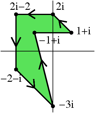
∫Something!e(e17z5(58z5 9z3+2)) dz
Well, let's try to make Something! a
more challenging curve. So: it will be a closed piecewise-linear
contour, from 1+i to 2i to 2i 2 to 2 i to 3i to 1+i to 1+i. This is
6 line segments, and a moderately bizarre function. Still, I can tell
you the value of this integral, and many, many others: the value is 0.
Of course I am concealing one of the most important results of the
course through excessive detail: this should be a major
intellectual crime. In fact, the setting has a name.
 Cauchy's Theorem
Suppose f is holomorphic in U, and C is a
closed curve in U whose interior is entirely in U. Then
∫Cf(z) dz=0.
Proof This is a major result in mathematics, and a large number
of people have spent a large amount of time over the last 150 years
making a verification of this result understandable. So here goes.
∫Cf(z) dz= ∫C(u(x,y)+i v(x,y))(dx+i dy)=
∫C(u(x,y)+i v(x,y))dx+(–v(x,y)+i u(x,y))dy.
What I used was (i)2=–1 and I reorganized the product
so that I have P(x,y)dx+Q(x,y)dy in preparation for using Green's
Theorem. I need to compute certain partial derivatives in order to get
the integrand for the double integral side of Green's Theorem.
Since P(x,y)=u(x,y)+i v(x,y), ∂P/∂y=∂u/∂y+i ∂v/∂y.
Since Q(x,y)=–v(x,y)+i u(x,y),
∂Q/∂x=–∂v/∂x+i ∂u/∂x.
The integrand in the double integral is
∂Q/∂x–∂P/∂y.
This is (–∂v/∂x+i ∂u/∂x
)
–
(∂u/∂y+i ∂v/∂y
).
We can rearrange this to get
(–∂v/∂x–∂u/∂y)
+i
(∂u/∂x–∂v/∂y
).
Each of these real and imaginary parts is 0. These conditions are
exactly the Cauchy-Riemann equations.
After 150 years, the proof should be easy, shouldn't
it?
zz
 I'll try to do this problem, remembering that our definition of
AB is eB log(A) (that's the small l version
of log and the distinction is important!). The useful diagram to the
left is the unit circle in the first quadrant. Of course, A is 1, B is
(1+i)/sqrt(2), and C is i. I'll define S(z)=zz -- S for
"superexponential".
I'll try to do this problem, remembering that our definition of
AB is eB log(A) (that's the small l version
of log and the distinction is important!). The useful diagram to the
left is the unit circle in the first quadrant. Of course, A is 1, B is
(1+i)/sqrt(2), and C is i. I'll define S(z)=zz -- S for
"superexponential".
a) What are all values of S(A), S(B), and S(C)?
The detailed results are perhaps slightly
surprising. For all of A, B, and C, ln(|z|)=ln(1)=1 which will
simplify things a
bit.
S(A)=e1 log(1)=e0+i arg(1). Now arg of
any non-zero complex number has infinitely many values, so we
almost expect confusion. But here arg(1)=2Πk where k is any
integer, positive or negative or 0, and exp is 2Πi periodic,
e0=1, so 11 has only one value, 1.
S(B)=[(1+i)/sqrt(2)](1+i)/sqrt(2)=e(1+i)/sqrt(2)[ln(1)+i arg((1+i)/sqrt(2))]=e(1+i)/sqrt(2)[ln(1)+i((Π/4)+2Πk)]=e–((Π/4sqrt(2))+2Πk/sqrt(2))ei(((Π/4)+2Πk)/sqrt(2)).
I write things this way because I hope to understand
eKei L if K and L are real numbers. In
particular, I can easily write the real and imaginary parts of the
complex number, since ei L is cos(L)+i sin(L). So
the values of S(B) are (e–((Π/4sqrt(2))+2Πk/sqrt(2))cos1(((Π/4)+2Πk)/sqrt(2))
)+i (e–((Π/4sqrt(2))+2Πk/sqrt(2))sin(((Π/4)+2Πk)/sqrt(2))
), a complicated mess.
The values of S(C) were a bit surprising to me:
ii=ei log(i)=ei[ln(|i|)+i arg(i)]
=e–Π/2–2Πk. All of the values are real.
b) If we start with k=0 at 1 and move along the curve so that
zz varies continuously -- this depends on the
value of arg selected. I would have been happy if students had
mentioned that Arg (capital A!) was continuous on the curve (in fact,
in the right half-plane, it is arctan(y/x), certainly
continuous. So the values of S(B) and S(C) are the values above with
k=0. Please note that if the circular arc were continued around to,
say, –i, then k=0 would not be correct! The value would not be
the "principle" value, but the value used when k=1. This is
complicated and either irritating or interesting.
c) What does the image of the curve under the mapping
z→S(z) look like? This is what I did:
S(z)=S(eit) for z on the curve, with 0≤t≤Π/2. Then
(eit)eit=eeit[log(eit)]=eeiti t
because Arg(eit) is just t for those points on the curve
and ln(|eit|)=ln(1)=0. Then
eeiti t=ei t[cos(t)+i sin(t)]=e–t sin(t)ei t cos(t)=e–t sin(t)cos(t cos(t))+ie–t sin(t)sin(t cos(t)).
I finally gave up and asked Maple which
produced the graph to the right. Superior people could probably have
drawn the graph with pure thought.
Please note that the "top" of this curve does not correspond to
S(B). The intercepts on the real axis are at 1 and
e–Π/2, the principal values of S(A) and S(C).
The frog ...
So here is the problem statement:
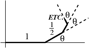
A frog starts at the origin. It leaps one unit eastward (to the
right!) on its first jump, 1/2 unit on its second, 1/4 unit on its
third, 1/8 on the fourth, and so on, each time turning
exactly an angle θ to the left from the previous jump. Assuming
only that 0<θ<Π, show that this frog will always end up
at some point on a semicircle of radius 2/3. Sketch this
semicircle.
So the hops of the frog are the sum of a series:
1+eiθ/2+e2iθ/4+e3iθ/8+...
The eiθ's rotate by the angle needed, and the
divisions by powers of 2 shrink the lengths of the leaps. Then this is
a geometric series with first term=1 and ratio between successive
terms equal to eiθ. The modulus of the ratio is 1/2
which is <1, so the series converges and its sum is
1/(1–eiθ/2).
I followed the solution of Ms. Addabbo
in what I told the class. My own solution was quite clumsy. So: she
set θ=0 and θ=Π to get points on the positive real
axis: 2 and 2/3. Then she guessed (?) that the semicircle would be
centered at 4/3 with radius 2/3. So all she needed to do was to show
that 1/(1–eiθ/2) has distance 2/3 from 4/3. So:
1 4 2 4 6–4(2–eiθ)
------- – --- = ------ – --- = ----------
1–eiθ/2 3 2–eiθ 3 6–3eiθ
The top becomes 2+4eiθ.
If we want the modulus of this to be 2/3, we could multiply the
fraction by 3/2 and verify that it has modulus 1. So:
The top becomes 6+12eiθ while the bottom becomes
12–6eiθ. Let's throw out the factors of 6 to get
1+2eiθ divided by 2–eiθ. But the
modulus of the top is the same as its product with
e–iθ. That is e–iθ+2. The complex
conjugate of that is eiθ+2, the bottom. So the
modulus of the quotient is equal to 1 (the quotient of w divided by w has modulus 1
because modulus of a quotient is the quotient of the moduli and the
modulus of the conjugate is the same as the modulus of the original
complex number).
This is certainly not clear to me. I will show you a much more
systematic way to analyze such things later in the course.
| Wednesday,
February 17 | (Lecture #8) |
|---|
Another way to compute some integrals
For example, suppose we have a curve, C, with z=x(t)+i y(t), for
t in [a,b]. Then dz=(x´(t)+i y´(t))dt, either by
differentiating that equation or by using dz=dx+i dy. If we want
to integrate z5 on this curve, 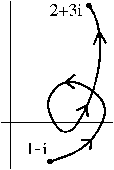 we could substitute and get
∫t=at=b(x(t)+i y(t))5
(x´(t)+i y´(t))dt.
But I know the Chain Rule: the
derivative of (1/6)(x(t)+i y(t))6 with respect to t is exactly (x(t)+i y(t))5
(x´(t)+i y´(t)). So I can antidifferentiate and plug
in. What I get is (1/6)(z at the end of C where t=b)6–(1/6)(z
at the start of C where t=a)6.
we could substitute and get
∫t=at=b(x(t)+i y(t))5
(x´(t)+i y´(t))dt.
But I know the Chain Rule: the
derivative of (1/6)(x(t)+i y(t))6 with respect to t is exactly (x(t)+i y(t))5
(x´(t)+i y´(t)). So I can antidifferentiate and plug
in. What I get is (1/6)(z at the end of C where t=b)6–(1/6)(z
at the start of C where t=a)6.
You may recognize this as a variation of one of the calc 3 methods for
computing a line integral (exact differentials and path
independence). But in practice it is easy: take
any curve W joining, say, 1–i and 2+3i. Then
∫Wz5dz=(1/6)(2+3i)6–(1/6)(1–i)6.
Very easy!
Estimating the size of complex line integrals
Many of our exact computations will depend on what seems like
sloppy overestimates of the modulus of complex line integrals. Let me
show you how this works, and then do a few examples. We'll have many
more examples later in the course! The explanation is a bit devious
and complicated, but the final result will be easy to use. I promise.
So I want to estimate I=∫Cf(z) dz where C is a
piecewise smooth curve and f(z) is continuous on the curve C. Well, I
is a complex number. If it isn't 0 (in which case estimating it is
rather easy) then there is θ so that ei θ
is real and positive. So now we know:
|∫Cf(z) dz|=ei θ∫Cf(z) dz=∫Cei θf(z) dz=∫t=at=bei θf(z)(x´(t)+i y´(t))dt
Now, wait! The quantities above are all real and positive. But "Re" is
linear and so is "∫". What I mean is the following: FROG and TOAD
are real functions, then Re(∫FROG+iTOAD) is
Re(∫FROG+i∫TOAD) which is Re(∫FROG). This is the same as
∫Re(FROG+iTOAD).
Since ∫t=at=bei θf(z)(x´(t)+i y´(t))dt
is real and positive, it is equal to its real part:
Re(∫t=at=bei θf(z)(x´(t)+i y´(t))dt)=∫t=at=bRe(ei θf(z)(x´(t)+i y´(t)))dt. But remember that the real part of
anything is ≤ the modulus, so this is ≤∫t=at=b|ei θf(z)(x´(t)+i y´(t))|dt.
What are we integrating?
|ei θf(z)(x´(t)+i y´(t))|
=|
ei θ| |f(z)| |x´(t)+i y´(t)|=|f(z)| sqrt(x´(t)2+ y´(t)2)
Now suppose some wonderful person tells me that |f(z)| is at most M on
the curve. Then the quantity above is at most
M sqrt(x´(t)2+ y´(t)2).
Don't panic -- we're almost done. So pasting together the very start
with this we get:
|∫Cf(z) dz|≤∫t=at=bM sqrt(x´(t)2+ y´(t)2)dt.
But the integral of that strange square root quantity is exactly the
length of the curve C. We have verified
(and won't ever think again about the tricky verification of):
The ML inequality
Suppose C is a piecewise smooth curve whose length is L, and suppose
that f(z) is a function which is continuous on C with modulus bounded
by M on C. Then
|∫Cf(z) dz|≤ML.
A few examples follow. These examples may seem strange, but they are
motivated by many aspects of complex analysis, as you will see.
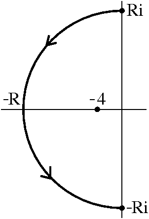 Example #1
Suppose f(z) is z2/(z+4) and C is the left half of a circle
of radius R centered at 0 where R is very large. C is oriented
counterclockwise, of course, the way it should be! Then
|f(z)|≤|z|2/(|z|–4). I choose to underestimate
|z–4| by |z|–4 rather than 4–|z| because I was told
that R=|z| is "large" and this way the underestimate is positive. This
is overestimated by M=R2/(R–4). The length of this
curve is, of course, L=ΠR. So my estimate is
ΠR3/(R–4).
Comment My pal Maple claims to
compute this integral exactly (I haven't done it!). I used the
Rei t parameterization and got a definite
integral. The incredibly silly exact value claimed is
8R+16Πi+16 ln({R–4}/{R+4}). So this is O(R) (big-oh of R, the order of increase
as R→∞). Our estimate is much "weaker": it is
O(R2).
Example #2
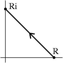 Here let's consider f(z)=ei z/z3 where C is
the line segment from the large positive real number R to the number
R i. The length of this line segment is L=sqrt(2)R. What about M?
Well, |f(z)|=|ei z|/|z|3. The bottom is
easy enough: it is R3. What can I say about
|ei z|? Realize, please, that if w=c+d i is a
complex number with real and imaginary parts c and d, respectively,
then ew=ecei d. The number
ei d is on the unit circle and so has modulus 1. And
therefore |ew|=eRe(w). Here we have
ei(x+i y), so the modulus is e–y. If
we realize that C is in the upper half-plane, then we know that
e–y≤e0=1. Therefore a valid M is
1/R3, and our ML estimate is just
sqrt(2)/R2. Immediately we see that the limit of
∫Cf(z) dz as R→∞ is 0. That's the sort
of behavior we'll want.
Here let's consider f(z)=ei z/z3 where C is
the line segment from the large positive real number R to the number
R i. The length of this line segment is L=sqrt(2)R. What about M?
Well, |f(z)|=|ei z|/|z|3. The bottom is
easy enough: it is R3. What can I say about
|ei z|? Realize, please, that if w=c+d i is a
complex number with real and imaginary parts c and d, respectively,
then ew=ecei d. The number
ei d is on the unit circle and so has modulus 1. And
therefore |ew|=eRe(w). Here we have
ei(x+i y), so the modulus is e–y. If
we realize that C is in the upper half-plane, then we know that
e–y≤e0=1. Therefore a valid M is
1/R3, and our ML estimate is just
sqrt(2)/R2. Immediately we see that the limit of
∫Cf(z) dz as R→∞ is 0. That's the sort
of behavior we'll want.
Comment How about "exact computation"? My pal Maple does not like this integral too
much. It claims, after some "thought", that its "value" is an
expression with 14 terms, several of which are some quite complicated
"special functions". Yes, they are hypergeometric functions, but more
elaborate than what I showed you. For example, one piece involves
values of 2F2(1,1;2,2;z)! Knowing this "exact
value" doesn't help me, at least, to understand that the limit as R
gets large will be 0. But such asymptotic information is important in
this subject.
We are now ready to start the course.
So we need to look at {f(z+Δz)–f(z)}/Δz and of course
consider what happens when Δz→0.
GOOD
Take f(z)=z2. Then, just as in times past (!) we see that
{f(z+Δz)–f(z)}/Δz is
{(z+Δz)2–z2}/Δz which becomes
2z+Δz. When Δz→0, this becomes 2z. Indeed, the limit
exists and is always 2z.
BAD
Let's try f(z)=z. I will
work with some cleverness. What happens if Δz is just
Δx, only a real "increment"? Well, (write z=x+i i)
f(z+Δz)=f((x+i y)+Δx)=x–i y+Δx, so
{f(z+Δz)–f(z)}=x–i y+Δx–(x–i y)=Δx. Then
the limit of the difference quotient will be 1.
Now let's try a "purely imaginery" Δz, so Δz is just
i Δy. What happens?
If z=x+i y,
f(z+Δz)=f((x+i y)+i Δy)=x–i y–i Δy, and the difference
quotient {f(z+Δz)–f(z)}/Δz becomes
{(x–i y–i Δy)–(x–i y)}/(iΔy) becomes
–1.
But this means that the limit of {f(z+Δz)–f(z)}/Δz does
not exist. This function is not complex differentiable!
What's going on? Apparantly the most modest requirement, that the
"obvious" limit of the difference quotient exists, throws out at least
one (and in fact, many!) nice-looking functions. Maybe a bit of
generality is useful here, a sort of overview.
Suppose we have a function which takes the complex number x+i y
to the complex number u(x,y)+i v(x,y). I want the limit of
(u(x+Δx,y+Δy)+i v(x+Δx,y+Δy))–(u(x,y)+i v(x,y))
-----------------------------------------------
Δx+iΔy
as Δx+iΔy→0 to exist. Let me temporarily call the
limit A+Bi. There are some obvious special cases to consider when
thinking about this limit similar to what I did during the second
example above.
- Set Δy=0 (a sort of horizontal limit). Then
if the limit exists (as Δx→0), it must be
(∂u/∂x)+i (∂v/∂x) because what's left are
just two limits with Δx's.
| 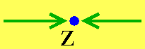 |
- Set Δx=0 (a vertical limit). Then if the limit
exists (as Δy→0), it must be (a bit of care because
there is another i in the bottom!)
(1/i)(∂u/∂y)+(∂v/∂y) because what's left are just
two limits with Δy's.
| 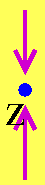 |
Now both of these are supposed to be the same complex number,
A+Bi. Two ways of writing A tell me that:
∂u/∂x=∂v/∂y
And then two ways of writing B tell me that (remember, 1/i is –i)
∂v/∂x=–∂u/∂y
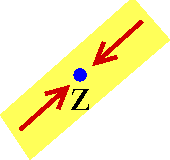 |
It is natural to wonder if there are any further "compatibility
conditions" that u and v need to satisfy. For example, we could
consider the limit where Δz=Δt+i Δt as
Δt→0 (a sort of diagonal limit) or
Δt+i (Δt)2 as Δt→0 (a sort of
limit along a parabolic path). There are results for both of these but
the results turn out to be linear combinations of the two already
obtained. In fact, for reasonable functions, there aren't any further
conditions.
| 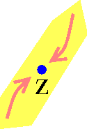 |
Theorem Suppose u(x,y) and v(x,y) have continuous first partial
derivatives. Then limΔz→0(u(x+Δx,y+Δy)+i v(x+Δx,y+Δy))–(u(x,y)+i v(x,y))/Δz exists exactly
when (o.k., "if and only if") ux=vy and
uy=–vx.
The partial differential equations ux=vy and
uy=–vx are called the Cauchy-Riemann equations.
Example
Let's try a fairly benign-looking function,
|z|2=x2+y2. In this case,
u(x,y)=x2+y2 and v(x,y)=0 (the zero function
whose value is 0 for all inputs). Then ux=vy and
uy=–vx become 2x=0 and 2y=0 so this
function is "complex differentiable" only when z=0!
Example
We tried u(x,y)=x2 and v(x,y)=2xy. Then (perhaps
remarkably!) the Cauchy-Riemann equations are always true, and
(x2–y2)+i(2xy) is always complex
differentiable. But maybe this isn't remarkable, since these functions
are the real and imaginary parts of z2.
Example
Now u(x,y)=excos(y) and v(x,y)=exsin(y). Here
the minus signs are neat, and again it turns out that the
Cauchy-Riemann equations are satisfied everywhere. Of course, this
function turns out to be ez.
| Monday,
February 15 | (Lecture #7) |
|---|
The most important tools
- Infinite series (especially power series)
- Line integrals
| Phrase | Proper definition | Possible
picture |
|---|
| The last two definitions (continuing from the
previous lecture) |
|---|
| Adding curves | Suppose C1(t) is a curve
with domain [a,b] and C2(t) is a curve with domain
[c,d]. If C1(b)=C2(c) (that is,
C1's "Head"=C2's "Tail", perhaps) then
the curve C(t) whose domain is [a,b+d–c] and defined by
C(t)=C1(t) if t<b and C(t)=C2(t–b+c) (I
hope!) is called the sum of C1 and C2. We
will write C=C1+C2. | 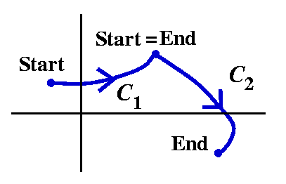 |
| Reversing curves
| If C(t) is a curve with domain [a,b], then the "reversal of
C(t)", also called –C, will be the curve, let me temporarily
call it D(t), whose domain will also be [a,b], defined by D(t)=C(b+a–t).
–C is just C backwards. The picture is slightly weird (how
should I have drawn it?) but I hope you get the idea.
| 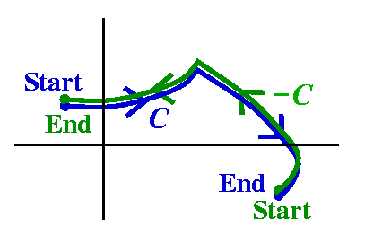 |
I hope the darn formulas for C1+C2 and –C
are correct. I don't think I will ever be so formal again in this
course. I will usually be rather casual. The curves in this course
will all be piecewise differentiable, and, actually, I think every
curve I'll consider will turn out to be sums of line segments and
circular arcs. So bah to
general theory!
The truth: parameterized curves
Actually I should acknowledge that what we are defining are called
parameterized curves. For example, the curves
C1(t)=3t+5t i for t in [0,4] and
C2(s)=3s2+5s2 i for s in [0,2]
are really different, but they "look" the same: the line
segment from 0 to 12+20i. But we will mostly be interested in line
integrals and it will turn out that the values of such integrals will
not depend upon parameterizations.
A few examples
This curve is a straight line segment starting at –4i and going to
–2i, followed by a quarter circle whose center seems to be 0,
starting at –2i and going to 2.
If I wanted to be totally strict, I guess I could define a C(t) on the
interval from [0,2+(Π/2)] Let's see: for t in [0,2), let C(t) be (t–4)i,
and for i in [2,2+(Π/2)], define C(t) to be
2ei(t–2–(Π/2)).
Some remarks
Almost always in this course I will parameterize
circles and circular arcs using the complex exponential. My first
guess will always be
CENTER+(RADIUS)e(i parameter).
Another remark: what I've just done is excessively precise and maybe
slightly silly. I want to write curves in a way that is convenient. So
this curve should be written as a sum of two curves, say
C1+C2. Here C1(t)=ti where t is in
the interval [–4Π,–2Π], and C2(t)=0+2eit where
t is in the interval [–Π/2,0]. It is just easier to do this than to
try to figure out the total length, how to combine and adjust
parameterizations, etc.
|  |
|
Here I will write the curve again as a sum,
C1+C2. C1 seems to be a semicircle of
radius 2 and center –1. It goes backwards. So
C1(t)=–1+2ei([Π]–t) where t is in the interval
[0,Π]. C2 is a straight line segment. This I know how to
parameterize from thinking about
convexity. C2(t)=(1–t)(1)+(t)(–3i) where t is in the
interval [0,1].
A remark
Parameterizing a circular arc in a clockwise fashion
feels close to obscene to me. Almost always in this course our circles
will be parameterized counterclockwise.
|  |
The definition
Now I want to define ∫CP(x,y)dx+Q(x,y)dy where P(x,y)
and Q(x,y) are at least continuous in an open set containing the curve
C. In fact, in this course, these functions will almost always be
differentiable. They will also almost always be rather explicit, as
will the curve C. So here is the official definition:
If C is the curve defined by x(t) and y(t) for t in [a,b],
then ∫CP(x,y) dx+Q(x,y) dy is defined to be
∫t=at=bP(x(t),y(t))x´(t)+Q(x(t),y(t))y´(t) dt.
This is of course valid if the curve is smooth. When the curve is
piecewise smooth, we break up the interval [a,b] into subintervals
where the functions are smooth, compute using the definition above in
each of the subintervals, and then add the result.
Now there's a serious difficulty, because line integrals were
originally developed to compute physical quantities which seemed to
only depend on the geometry of the situation and the values of P and Q
(the simplest examples are work and flux). But the definition we
wrote has a dependence on the parameter, which makes no sense
physically. Let's look at a specific case more closely. For simplicity
I will write things only with real functions. "Complexifying" the line
integrals will cause no difficulty and we'll do it later.
 We connect the point (0,0) and (12,20) with a straight line
segment. This can be parameterized in many ways. Let me look at the
two we previously mentioned.
We connect the point (0,0) and (12,20) with a straight line
segment. This can be parameterized in many ways. Let me look at the
two we previously mentioned.
- Here the C1 parameterization is given by x(t)=3t
and y(t)=5t for t on [0,4]. Then
&intC1P(x,y) dx+Q(x,y) dy becomes
∫04{P(3t,5t)3+Q(3t,5t)5}dt.
- Here the C2 parameterization is given by
x(s)=3s2 and y(s)=5s for s on [0,2]. Then
&intC2P(x,y) dx+Q(x,y) dy becomes
∫02{P(3s2,5s2)6s+Q(3s2,5s2)10s}ds.
What's the relationship between ∫04{P(3t,5t)3+Q(3t,5t)5}dt
and ∫02{P(3s2,5s2)6s+Q(3s2,5s2)10s}ds?
In fact, they are the same! If t=s2, then dt=2s ds,
and the s-interval [0,2] becomes the t-interval [0,4]. The P and Q
values coincide so the results are the same. A general verification
is similar to this.
The value of a line integral does not
depend on parameterization.
Further properties of line integrals
The following "linearity" results are easy, and have been covered in
calc 3:
Additivity ∫C1+C2P(x,y) dx+Q(x,y) dy=∫C1P(x,y) dx+Q(x,y) dy+∫C2P(x,y) dx+Q(x,y) dy
Reversal ∫–CP(x,y) dx+Q(x,y) dy=–∫CP(x,y) dx+Q(x,y) dy
Green's Theorem
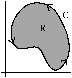 The major result in the subject is Green's Theorem which connects
line integrals to double integrals. The hypotheses are rather important
in both applications (electromagnetism) and theory (complex
variables). Here we go:
The major result in the subject is Green's Theorem which connects
line integrals to double integrals. The hypotheses are rather important
in both applications (electromagnetism) and theory (complex
variables). Here we go:
Green's Theorem
Suppose C is a simple closed piecewise smooth curve which
is the boundary of a connected open set R. C is parameterized so that
the increasing values of the parameter have R to the left. Suppose
P(x,y) and Q(x,y) are continuously differentiable functions of two
variables at all points of both R and C. Then
∫CP(x,y) dx+Q(x,y) dy=∫∫R{∂Q/∂x}–{∂P/∂y} dAx,y.
The dAx,y is to remind me that x and y are the variables in
the functions, and, as needed, dAx,y could be replaced by
dx dy or dy dx or even other things (for example, double
integrals in polar coordinates use r dr dθ).
Some of the phrases in this result will occur again and again in this
course. There are abbreviations for them. For example, a "connected
open set" will be called a domain. And "C is parameterized so
that the increasing values of the parameter have R to the left" will
be called the boundary of R is oriented positively (actually,
we probably won't even mention this most of the time, because
essentially every boundary curve will be oriented positively).
People have made careers out of proving various versions of Green's
Theorem with slightly weakened hypotheses (some of these have been
moticated by authentic applications in physics, though). A realistic
version of Green's Theorem, as quoted above, would probably take 3 or
4 lectures to prove but I'd like to verify some specific
version because this gives an idea of what's going on.
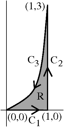 I'll specify the boundary of the domain first. I want it to be roughly
triangular in shape, but let me make one part of the boundary curved
so some small difficulty will occur. Here we go: the boundary will be a
straight line segment connecting (0,0) to (1,0), and then a straight
line segment connecting (1,0) to (1,3), and then from (1,3) to (0,0),
the curve y=3x4. The domain R is what's inside. So I want
to connect the double integral to the line integrals.
Let me consider first the line integrals over the boundary. There are
three chunks of boundary, and I will analyze each of them.
I'll specify the boundary of the domain first. I want it to be roughly
triangular in shape, but let me make one part of the boundary curved
so some small difficulty will occur. Here we go: the boundary will be a
straight line segment connecting (0,0) to (1,0), and then a straight
line segment connecting (1,0) to (1,3), and then from (1,3) to (0,0),
the curve y=3x4. The domain R is what's inside. So I want
to connect the double integral to the line integrals.
Let me consider first the line integrals over the boundary. There are
three chunks of boundary, and I will analyze each of them.
- C1, the straight line segment connecting (0,0) and
(1,0).
So here I will use v=x as my parameter. v varies from 0 to 1. Notice that
y=0 always here, so that
∫C1P(x,y) dx+Q(x,y) dy becomes
∫01P(v,0) dv (the Q term drops out
because the derivative of 0 is 0).
- C2, the straight line segment connecting (1,0) and
(1,3).
Here use q=y as the parameter, going from 0 to 3. Of course x=1 always,
so its derivative will be 0 and now the P term goes away. Now
∫C2P(x,y) dx+Q(x,y) dy is
∫03Q(1,q) dq.
- C3, the curve y=3x4 oriented from (1,3) to
(0,0).
I'll compute it from (0,0) to (1,3) and then multiply by
–1. Since y=3x4, I can parameterize by x=w and
y=3w4 with w going from 0 to 1. Then
∫–C3P(x,y) dx+Q(x,y) dy is
∫01P(w,3w4)+Q(w,3w4)12w3 dw
and what we need is minus that.
So one side of Green's Theorem is
∫01P(v,0) dv+∫03Q(1,q) dq–(∫01P(w,3w4)+Q(w,3w4)12w3 dw).
If I reorganize a bit, some of the mystery will disappear. There's a P
part and a Q part.
∫01P(v,0) dv–∫01P(w,3w4) dw+∫03Q(1,q) dq–∫01Q(w,3w4)12w3 dw.
Let me recognize (?) the P part first. The "variable of integration"
is a dummy variable. I can rename them both in any way I desire. So I
will change both v and w to x. Then I'll combine integrals.
∫01P(v,0) dv–∫01P(w,3w4) dw=∫01P(x,0)–P(x,3x4) dx.
What is this? Mr. Green would have us believe this is related to a
double integral,
∫∫R{∂Q/∂x}–{∂P/∂y} dAx,y.
Let's again just select the P part. So I have
∫∫R–{∂P/∂y} dAx,y.
Now I will be clever, very clever. I choose to replace
dAx,y by dy dx. So I am officially converting this
double integral to an iterated integral. Of course, the limits of the
integrals need to be found, but the region is not very
complicated. The iterated integral is
∫x=0x=1∫y=0y=3x4–{∂P/∂y} dy dx.
Consider the inside integral,
∫y=0y=3x4–{∂P/∂y} dy.
I am integrating dy something which is a derivative with respect to
y. The Fundamental Theorem of Calculus applies and
∫y=0y=3x4–{∂P/∂y} dy=–P(x,y)]y=0y=3x4=P(x,0)–P(x,3x4)
(I hope I did the signs correctly!). This I put back in the "outer"
integral and I get
∫x=0x=1{P(x,0)–P(x,3x4)} dx
No accident, this matches the P part of the line integral side of
Green's Theorem.
If we start with the Q part of the double integral (I'll go the other
way just for fun), then
∫∫R{∂Q/∂x} dAx,y=∫y=0y=3∫x=y1/4/3x=1{∂Q/∂x} dx dy=∫y=0y=3Q(x,y)]x=y1/4/3x=1 dy=∫y=0y=3Q(1,y)–Q(y1/4/3,y) dy.
So we have
∫y=0y=3Q(1,y)–Q(y1/4/3,y) dy
and should match that somehow with the line integral contribution,
∫03Q(1,q) dq–∫01Q(w,3w4)12w3 dw.
The first part of each expression has equal values. But why should
∫y=0y=3Q(y1/4/3,y) dy and
∫01Q(w,3w4)12w3 dw
be equal? Make the substitution y=3w4 in the second
integral and follow through the limits and dy=12w3dw
etc. They are the same!
We have proved Green's Theorem for this region and its boundary. I
hope you see where we needed to know about P and Q on the boundary
and at every point inside. Just omitting the hypotheses at one
interior point has profound consequences both practical (electric
charges!) and theoretical (we'll see this!).
About George Green
George Green lived from 1793 to 1841. Biographical information is
available here
and here.
Some aspects of his adult life were quite unconventional, but perhaps
more interesting is that (quoted from the first link), "The younger
Green only had about one year of formal schooling as a child, between
the ages of 8 and 9." Later, in 1832, nearly 40 years old (!), he
"went to college" (Cambridge). A version of his original 1828
publication, An Essay on the Application of mathematical Analysis
to the theories of Electricity and Magnetism. (83 pages), is
available here if you
have the curiosity and courage to look at it. Almost every page is
dominated by physical discussions. A modern advanced point of
view is in the book Calculus on Manifolds by Michael Spivak
(not an easy book, almost formidably abstract and mathematical,
perhaps a counterbalance to Green's original essay).
Complex line integrals
Everything works. What do I mean? Let me take one of our previous
examples, shown again to the right, and call it C. I want to actually
compute the integral
∫C3x2–i y dz. The only
abbreviation I need to tell you is that dz means dx+i dy. So we
want to compute
∫C(3x2–i y)(dx+i dy) which
is
∫C(3x2–i y)dx+(y+i 3x2)dy.
We write C as C1+C2 where
C1(t)=i t for t in the interval
[–4Π,–2Π], and
C2(t)=0+2eit for t in the interval
[–Π/2,0]
- The C1 integral
Here x=0, dx=0, y=t, and dy=dt. Therefore
∫C1(3x2–i y)dx+(y+i 3x2)dy=∫–4Π–2Πt dt=t2/2]–4Π–2Π=–6Π2.
- The C2 integral
Here z=2eit=2cos(t)+2i sin(t) for
t in the interval [–Π/2,0], so that x=2cos(t),
dx=–2sin(t) dt,
y=2sin(t), and dy=2cos(t) dt. We translate:
∫C2(3x2–i y)dx+(y+i 3x2)dy=
∫–Π/20I'm tired.
I think I will let "interested people" (of which there are probably
none!) finish this computation. We are not going to do almost any
integrals this way. We will use different methods, maybe more
sophisticated.
| Monday,
February 8 | (Lecture #6) |
|---|
The most important tools
- Infinite series (especially power series)
- Line integrals
Today I hope to offer you an introduction and review of both. There
will be much about power series later in the course. It is the primary
tool for studying the local behavior of functions (how the
function behaves close to a given point). Line integrals are used to
state and verify many of the important basic results in the
subject. They also tend to give more global information.
Infinite series
Everything is similar to what was done in calc 2. In the text this
material begins on page 37. An infinite series is a sum of the form
∑j=1∞zj. Associated to this
"sum" is a sequence, the sequence of partial sums:
sn=∑j=1nzj. If the
sequence {sn} converges and its limit is s, then we
declare: the infinite series
∑j=1∞zj converges and its
sum is s. We're not computing infinitely many additions (!) --
we are trying to get the limit of a sequence.
Taking real and imaginary parts is linear, certainly for finite
sums. This leads to a series version of the fact
above.
Series Fact A complex series converges exactly when
both of the real series gotten from the real and imaginary
parts of the series terms converge. The sum of the complex
series is the sum of the sum of the series obtained from the real
parts plus i multiplied by the sum of the series obtained from the
imaginary parts.
Random infinite series don't have nice formulas for partial sums. The
best and most frequently used example of an infinite series with nice
formulas for everything is the geometric series. Things work exactly
as they do with the real version. Here is a very rapid review.
If r≠1, then
a+ar+ar2+...+arn=(a–arn+1)/(1–r). This
is proved by multiplying things by 1–r and noticing the
cancellations. Both a and r may be complex. Now if |r|<1, we know
that limn→∞rn=0. Therefore, since the
finite sum is a partial sum of the whole geometric series, we have
proved:
Convergent geometric series
If a is a complex number and r is a complex number with modulus <1,
then ∑j=0∞arj–1 converges,
and its sum is a/(1–r).
Example
Every series in this course will be related to this result. Here is a
silly but still amazing example. Suppose we want the sum of the series
cos(Π/6)/3+cos(2Π/6)/32+cos(3Π/6)/33+cos(4Π/6)/34+...,
that is,
∑j=1∞cos(jΠ/6)/3j. I
just asked Maple and got 7/146+(12/73)sqrt(3) as the answer. How did
the darn program get this? Maybe I won't want to do the details
myself, but I really would like to get an idea of the
method. Please consider what follows.
Well, cos(jΠ/6)/3j is the real part of
ei jΠ/6/3j which is the same as (ei Π/6/3)j. This is a geometric series with
first term ei Π/6/3 and ratio
ei Π/6/3. The modulus of this is 1/3 and since this
is less than 1, the series converges. Its sum is
(ei Π/6/3)/(1–ei Π/6/3).
But ei Π/6=sqrt(3)/2+i/2 (I know some friendly
triangles!), so that
(ei Π/6/3)/(1–ei Π/6/3) is
(sqrt(3)+i)/2 on top and 3–(sqrt(3)+i)/2 on the bottom. If then one
takes the real part and rearranges things, the result is,
indeed, indeed, ... 7/146+(12/73)sqrt(3). Really.
To me this is both impressive and absurd.
Absolute convergence
A series ∑j=1∞zj converges
absolutely if the series of real non-negative numbers
∑j=1∞|zj| converges.
In calc 2, the following fact is used: if a real series
converges absolutely, then it converges. Of course, almost immediately
the instructor asserts that the converse is not correct, and the
example exhibited is almost always the Alternating Harmonic Series,
∑j=1∞(–1)j/j. This series
converges by the Alternating Series Test (terms alternate in sign,
decrease in value, and actually have limit 0). The "absolute" series
corresponding to this is the Harmonic Series,
∑j=1∞1/j, which diverges (either use
the Integral Test, or examine the series in bigger and bigger blocks
of powers of 2, comparing it to a divergent series).
In fact, for complex numbers, absolute convergence also implies
convergence. Why? Well, if
∑j=1∞|zj| converges, then both
∑j=1∞|Re(zj| and
∑j=1∞|Im(zj| must converge (these
are real series and I am using the real comparison test
on them!). Since ∑j=1∞|Re(zj|
converges, then (using the calc 2 result!)
∑j=1∞Re(zj) must
converge. Similar logic for the imaginary part tells us that
∑j=1∞Im(zj) must converge. But
since the real and imaginary parts both converge, we then deduce that
∑j=1∞zj converges. So:
Absolute convergence implies convergence for complex series:
If
∑j=1∞|zj| converges, then
∑j=1∞zj converges.
In this course, essentially every series of interest will be
absolutely convergent (you will soon see why!). Questions about
"conditional convergence" of complex series are sometimes interesting
but very difficult to resolve. So, for example, If
{θj} is any sequence of real
numbers, then the series
∑j=1∞ei θj/j2
converges because it converges absolutely (compare the series of the
moduli to the p-series with p=2>1). The arguments of
the terms, the θj's, don't matter at all in
this. But, truly, I don't know any neat general "theorem" advising me
about {con|di}vergence of
∑j=1∞ei θj/j. I
know a few interesting partial results. They are complicated.
The Ratio and Root Tests are still valid for complex series. Their
verification proceeds in much the same way as what we just did. So if
we consider a series ∑j=1∞zj of
non-zero complex numbers (non-zero so I don't need to worry in what
follows about division by 0) then:
-
Root Test If
limj→∞|cj+1|/|cj|=r
exists, then when 0≤r<1, the original series converges
absolutely and therefore must converge.
-
Ratio Test If
limj→∞|cj|1/j=r exists
(the roots here are the usual non-negative roots of a non-negative
real number), then when 0≤r<1, the original series converges
absolutely and therefore must converge.
Of course, the irritation is that neither limit may exist (examples
are easy and are in calculus books) and that no information on
{con|di}vergence may be inferred in either case if r=1 (easy examples
again in calculus books). Section 1.4, problems 42 and 43, have hints
discussing verification of these two results.
Here are some typical examples. They occur as solutions of certain
differential equations but also in many other situations.
Classical example #1
∑j=0∞(–1)jz2j/[2jj!]2
I am not making this up. This is J0(z), the first Bessel
function of order 0. It converges absolutely and therefore converges
for all complex numbers, z. Such functions satisfy an ordinary
differential equation:
x2y´´+xy +(x2–ν2)y=0. Here
ν=0.
The Ratio Test (which I always think of first when I see
factorials) immediately (well, after some cancellations!) shows that
this series converges for all complex numbers z. Here is a bit more
information.
If
cj=(–1)jz2j/[2jj!]2
then |cj|=|z|2j/[2jj!]2
since the minus 1's drop out and the modulus filters through to the
z's. Then:
|cj+1| |z|2(j+1)/[2(j+1)(j+1)!]2 |z|2(j+1)[2jj!]2
------ = ------------------------- = ---------------------
|cj| |z|2j/[2jj!]2 [2(j+1)(j+1)!]2|z|2j
Now do things like (j=1)!=(j+1)j!, 2(j+1)=2j2, and
|z|2(j+1)=|z|2j|z|2. If you cancel
everything (?) the resulting quotient should be
|z|2/[22(j+1)2]. Now with |z| fixed,
as j→∞, this will →0 for all z's. The series converges
absolutely for all z, and therefore must converge for all z.
Classical example #2
The hypergeometric function 2F1(a,b;c;z) is a
(not) well-known example of a collection of functions discovered(?) by
Gauss and widely studied and generalized in the last hundred
years. Indeed, even now these functions are objects of intense
investigation. This is the traditional notation. Here it means the
function which, near z=0, is defined by the following series:
a·b a(a+1)·b(b+1) a(a+1)(a+2)·b(b+1)(b+2)
1+ ----- z + --------------- z2 + ------------------------- z3 + ....
1!c 2!c(c+1) 3!c(c+1)(c+2)
There is notation for the things appearing in this series, but I don't
want to worry you so I won't introduce the notation. I am not an expert on hypergeometric functions
(Rutgers does have some of them, though!). These functions occur in
numerous applications. In case you think I'm joking, here's
a reference. There are more than a quarter million Google links to the
query hypergeometric function. Most prominently, these
functions are solutions of
x(1–x)y´´+[c–(a+b+1)x] y´–a b y=0,
the
hypergeometric differential equation.
Let's look at an example, 2F1(1,2;3;z). What
is this? So a=1, b=2, and c=3 and the series above becomes
1·2 1(1+1)·2(2+1) 1(1+1)(1+2)·2(2+1)(2+2)
1+ ----- z + --------------- z2 + ------------------------- z3 + ....
1!3 2!3(3+1) 3!3(3+1)(3+2)
Let's see: this is
1·2 1(2)·2(3) 1(2)(3)·2(3)(4)
1+ ----- z + ----------- z2 + ----------------- z3 + ....
1!3 2!3(4) 3!3(4)(5)
which simplifies to
2 2 2
1+ --- z + --- z2 + --- z3 + ....
3 4 5
and so this is
∑j=1∞{2/(j+2)}zj. We could
try the Ratio Test again successfully, but let me try the Root
Test. We need to look at the jth root of the modulus of the
jth term. The result is
{21/j/(j+2)1/j}|z|. You may remember that if
α is real and positive, then
limj→∞α1/j=1. Also,
limj→∞j1/j=1. To verify these
equalities, take logs and limits and the exponentiate back (use L'H on
the second limit). Now (j+2)1/j=((j+2)1/{j+2})(j+2)/j and the result as j→∞ is
again 1. Therefore the limit is |z|. We see that this series converges
absolutely for |z|<1 and diverges for |z|>1. The radius of
convergence is 1. Even for this simple a series, the behavior of
the infinite series on the boundary of the "disc of convergence" is
quite complicated.
In general, you'll see that a power series will have a radius of
convergence and a disc of convergence with that radius. The
series will converge (because it will converge absolutely) inside the
disc. For z's not on the boundary but outside the disc, the series
will diverge. For various reasons, we won't be too interested in what
happens exactly on the boundary.
The book I mentioned
The "book" (reason for the quotes: there's not much of a plot, but
lots of background characters!) I mentioned in class is Handbook of
Mathematical Functions: with Formulas, Graphs, and Mathematical
Tables edited by Milton Abramowitz and Irene A. Stegun. It is
$26.37 from Amazon (Dover reprint), and has 1,046 pages. I bought it
because I wanted to be respectable. I know less than .01% of the
contents. You should read the reviews at Amazon before purchasing a
copy. It has lots of "stuff" in it, almost surely more than you would
want to know about a lot of things. It has many formulas. It is more
fun than ... than ... well, maybe there's no good end to such a
sentence. But once in a while reading it is both entertaining and
informative.
Let's go on to discuss the other major tool in the course, line
integrals.
Line integrals are integrals over curves in the plane. So I'll recite
the standard curve vocabulary first.
| Phrase | Proper definition | Possible
picture |
|---|
| Curve
| A curve is a function whose domain is an interval, [a,b], in
R, and whose range is in C. If C(t) is the curve, we could write
C(t)=x(t)+iy(t). In this course, these functions will generally be at
least continuous.
|  |
| Smooth (differentiable) curve
| C(t)=x(t)+iy(t) should be differentiable, so that x(t) and
y(t) are differentiable. Such a curve has a nice tangent vector at
every point.
|  |
| Piecewise smooth curve
| The curve C(t) is certainly continuous. But
additionally, we can divide the interval [a,b] into a finite number of
pieces, and in each of these subintervals C(t) is smooth. This will
allow us to take care of curves with finite numbers of corners, for
example.
| 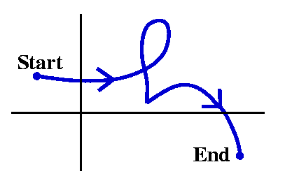 |
| Simple curve
| A simple curve is one which does not intersect itself
(except maybe: see the next plus one
definition). So if the
domain of C(t) is [a,b], and if a≤s<t≤b, then C(s) is
not equal to C(t).
| 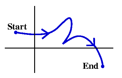 |
| Closed curve
| "Head=Tail" -- that is, if the domain of C(t) is {a,b], then
C(a)=C(b).
| 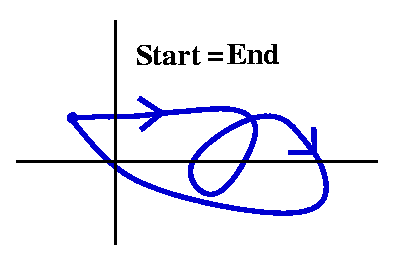 |
| Simple closed curve
| A closed curve which is also as simple as it can be(!). Here
C(a)=C(b), and C(s)=C(t) with
s<t implies either s=t or a=s and b=t.
| 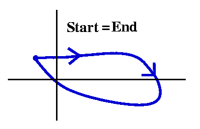 |
|
I stopped here. I'll continue next time with the two definitions
below and then do some examples and go on to line integrals.
|
|
| Adding curves | Suppose C1(t) is a curve
with domain [a,b] and C2(t) is a curve with domain
[c,d]. If C1(b)=C2(c) (that is,
C1's "Head"=C2's "Tail", perhaps) then
the curve C(t) whose domain is [a,b+d–c] and defined by
C(t)=C1(t) if t<b and C(t)=C2(t–b+c) (I
hope!) is called the sum of C1 and C2. We
will write C=C1+C2. | |
| Reversing curves
| If C(t) is a curve with domain [a,b], then the "reversal of
C(t)", also called –C, will be the curve, let me temporarily
call it D(t), whose domain will also be [a,b], defined by D(t)=C(b+a–t).
–C is just C backwards. The picture is slightly weird (how
should I have drawn it?) but I hope you get the idea.
| |
I hope the darn formulas for C1+C2 and –C(t) are
correct. I don't think I will ever be so formal again in this
course. I will usually be rather casual. The curves in this course
will all be piecewise differentiable, and, actually, I think every
curve I'll consider will turn out to be sums of line segments and
circular arcs. So bah to
general theory!
| Wednesday,
February 3 | (Lecture #5) |
|---|
Postponed!
I want to postpone the due
date of the second homework assignment
until the beginning of class on Wednesday, February 10, 2010.
Inequalities and complex numbers
So grading of your first formal homework assignment is ongoing. Even
now, thousands of instructors are passing the papers from hand to
hand, each evaluating every problem. Well, no: that's not quite
correct. I've read solutions to problems A and B, and to the first
textbook problem, and a grader will read the solutions to the other 5
textbook problems. It has been my experience with this course that the
first real challenge to students is consideration of
inequalities. Working with inequalities is the heart of
analysis. The additional emphasis in this course is that we have
complex algebra also on display. Let's review a few things about
inequalities.
First, inequalities are really a shorthand way of dealing with
positive quantities. People have recognized the following rules
about positive numbers:
- If w is a number, then w is positive, –w is positive, or w
is 0. Exactly one of these alternatives is true. (We abbreviate
the statement "w is positive" by the notation "w>0".)
- The sum of positive numbers is positive.
- The product of positive numbers is positive.
These are the only "rules" needed, and essentially everything else
involving manipulation of inequalities can be deduced from them. For
example, I will now deduce that 1, the multiplicative identity,
is positive. We know that 1≠0, and therefore by the first rule
above, either 1 is positive or –1 is positive. If –1 is positive, then
the product of –1 with itself is positive, but that is 1, so we have a
contradiction. So indeed, 1 must be positive. Our deduction is
done.
Now consider the complex numbers. The most interesting "new" number is
i. If we have the rules above are correct, then i is 0 or i is
positive or –i is positive. Certainly i is not 0 since its
product with itself is –1, which isn't 0. If i were positive,
then –1, the product of i with itself, would have to be
positive. But we just saw that couldn't be true. If –i were
positive, then the product of –i with itself would have to be
positive, but that also is –1. All three alternatives seem to be
impossible!
The correct conclusion is that there is no possible way to
define a collection of positive complex numbers. There is no
possible way to do inequalities with complex numbers
themselves. Therefore, when I am grading homework problems or exam
problems, if I see things like "5+6i> 2–i" or "w is a complex
number and 5w+2>–4" then I can STOP
READING. Any logical deductions which follow from such
assumptions are dubious. They may or may not be true as logical
statements but they certainly don't follow using any standard
argument. You must convert complex numbers into real numbers in
order to make valid statements using inequalities. The standard
mechanisms use modulus or real part or imaginary part, but
something has to be done. Bare statements with complex numbers and
inequalities contain no information.
De Moivre
The result (cos(θ)+i sin(θ))n=cos(nθ)+i sin(nθ) now
becomes (eiθ)n=ei nθ
which doesn't look so dramatic. I will usually write a complex number
of modulus 1 in this course as
ei(something real): this is easy and
compact.
|
AB
In this course, if A and B are complex numbers, we define
AB to be exp(A log(B)) which is usually written as
eA log(B). Note the small "l" in log. Since log can
have infinitely many values (because arg can have infinitely many
values), the symbol AB can also may have infinitely many
values.
A computation
For example, let's compute (1–i)3i. This should be
e3i log(1–i). But log(1–i) is
log(|1–i|)+i arg(1–i). Now log(|1–i|)=log(sqrt(2)),
not so hard. But 1–i is in the fourth quadrant, and its Arg is
–Π/4 so that arg(1–i) is –Π/4+2Πk where k is some
integer (positive or negative or zero). Therefore (1–i)3i is
e3i(log(sqrt(2))+i{–Π/4+2Πk})
which is
e(3Π/4+6Πk)+3log(sqrt(2))i.
This is
e(3Π/4+6Πk)cos(3log(sqrt(2)))+i e(–Π/4+6Πk)sin(3log(sqrt(2))).
When I ask Maple to compute
(1–i)3i, the result is
e(3Π/4)cos(3log(sqrt(2)))+i e(–Π/4)sin(3log(sqrt(2)))
so it seems to use "our" Arg.
z2
Integer powers work out well with this definition of
AB. For example,
z2=exp(2log(z))=exp(2{ln|z|+i(arg(z)+2Πk)})=exp(ln(|z|2)+i(2arg(z)+2Πk))=exp(ln(|z2|)+i arg(z2))=z2
because exp is 2Πi periodic and modulus and argument work well with
multiplication.
Back to abstraction ...
We need to discuss the foundational concepts of convergence and
continuity. Convergence will be needed for both sequences and
series. Continuity will be applied to functions. It is convenient to
have this language. I will mostly be repeating things you can read
about in section 1.4 of the text. Also, I'll just describe how to
support complex computations with the corresponding real computations
of calc 2.
If
p is a complex number, then |Re(p)|≤|p| and |Im(p)|≤|p|.
This means that if the complex number p has small modulus, then both
the real and imaginary parts of p are small. On the other hand,
the Δ≤ (the Triangle Inequality!) tells me
|p|≤|Re(p)|+|Im(p)|
so that if p has small real and imaginary parts, then the modulus of p
is small.
Convergence of a sequence of complex numbers
This is on page 33. If {zn} is a sequence of complex
numbers, we will say that {zn} converges to the complex
number A if |zn–A| gets small and stays small when n is
sufficiently large.
If you wish, I could be more precise: given any positive number,
ε, then there is a positive integer, N, so that if n≥N,
then |zn–A|<ε. The definition in this precision
is quite famous, and took much effort by the 19th century
mathematical establishment to formulate. If you are interesting in
investigating such statements, take 311, 411, 501, ... I will be
content if you really believe "gets close and stays close".
Further, if {zn} converges to A, then we also write
limn→∞zn=A or, sometimes,
zn→A.
You should notice that:
- If we consider the sequence {zn} and we know that
limn→∞zn=A, then, since
|Re(zn)–Re(A)|≤|zn–A| and
|Im(zn)–Im(A)|≤|zn–A|, we know
that the sequence of real numbers {Re(zn)} converges with
limit Re(A) and we know that the sequence of real numbers
{Im(zn)} converges with limit Im(A). So both of the real
sequences converge, and the limits have the "correct" connection to
the limit of the complex sequence.
- Again we start with a complex sequence {zn}. From it we
get two real sequences to consider: {Re(zn)} and
{Im(zn)}. It may happen that both of these sequences
converge. So suppose we know that
limn→∞Re(zn)=P and
limn→∞Im(zn)=Q for suitable real
numbers P and Q. Then I claim that
limn→∞zn=P+i Q. Why is this
true? Well, if |Re(zn)–P| is small and
|Im(zn)–Q| is small then
|zn–(P+i Q)|≤|Re(zn)–P|+|Im(zn)–Q|
so |zn–(P+i Q)| is small, and
limn→∞zn=P+i Q.
Here is the enormously useful fact we've learned:
Fact A complex sequence converges exactly
when both of the real sequences gotten from the real and imaginary
parts of the sequence elements converge. The limit of the complex
sequence is the sum of the limit of the real parts plus i multiplied
by the limit of the imaginary parts.
I'm going to use the Fact to take all the information I can
about real sequences and create results about complex
sequences. Before I do that, let's see if you understand some of the
remaining difficulties. Because I could also "convert" a complex
sequence into a pair of real sequences by using the polar
representation. So we could have {zn} and then contrast the
sequences {|zn|} and {arg(zn)}. But
arg(zn) isn't a real number: it is a set of real numbers!
So maybe we should look at the connection between convergence of
{zn} with the convergence of the pair of real sequences
{|zn|} and {Arg(zn)}. There are two sorts of
implications.
- Suppose {zn} converges. What can we say about
{|zn|} and {Arg(zn)}? Well,
|zn|–|A|≤|zn–A| and
|A|–|zn|≤|zn–A| by our "reverse" triangle
inequality. But this means ||zn|–|A||≤|zn–A| (no matter which one of
|zn| or |A| is larger!). But this means {|zn|}
converges and that its limit is |A|. So the convergence of one of the
real sequences is just about clear. Must the sequence
{Arg(zn} also converge? Polar coordinates can sometimes be
rather irritating, and this is an example. Remember that Arg of a
complex number is the unique argument in the interval
[–Π,Π). There must be trouble near the negative
real axis. For example, consider the sequence given by
zn=–1+(–1)n(i/n). I know this sequence converges:
its real parts are all –1; the imaginary part of the
nth term has absolute value 1/n, so those →0. The
sequence converges and its limit is –1. The arguments certainly
→1, because sqrt(1+{1/n2})→1. But what about
Arg(zn)? For n odd, (–1)n is –1, and
zn is in the lower halfplane, with
Arg(zn)→–Π. For n odd, the terms are in the upper
halfplane, and since they approach –1 on the negative real axis, this
subsequence of Arg's must →Π/2. This is annoying. In fact, if
the limit of the complex sequence {zn} is not on the
negative real axis, then sequence of {Arg(zn)} does
"behave" and it has a limit which is Arg of the limit fo the complex
sequence (this is seen using the calculus arctan function). I'm not
interested in the details: I'll just try to avoid arguments with Args.
- Suppose {zn} is a sequence of complex numbers and we
know both {|zn|} and {Arg(zn)} converge. Then
since both sine and cosine are continuous, I know that
|zn|ei Arg(zn)=|zn|cos(Arg(zn))+i |zn|sin(Arg(zn))
converges. Wow! In fact, let me push this a bit
more. Sometimes we can conclude that {zn} converges
only knowing about the convergence of one of the sequences
{|zn|} and {Arg(zn)}. Can you see which one, and
under what additional circumstance?
I hope the assertion is the following: if we know that
limn→∞|zn|=0 then the sequence
{zn} must also converge and its limit will be 0. This is
because the values of sine and cosine applied to various Args must be
in [–1,1] so the product and sum will →0.
We'll have many sequences which converge to 0. Such sequences occur
when we investigate infinite series. So if Q is a complex number with
|Q|<1, the sequence {Qn} converges to 0 since I know the
real sequence {|Q|n} converges to 0. And, more weirdly,
perhaps, would be defined by zn=(3+4i)n/n!. This
sequence converges to 0 because the real sequence {|zn|}
which is {5n/n!} has limit 0 (factorials grow much faster
than any powers!).
Continuity
A continuous function transforms convergent sequences to
convergent sequences. I mean: if {zn} is any convergent
sequence in the domain of the function f and if A, the limit of the
sequence, is also in the domain of f, then the sequence
{f(zn)} must also converge, and its limit will be f(A).
(There are other definitions of continuity, but, again, this won't
turn out to be a major technicality in this course. [What will
be, then?])
Almost every function in this course will be an example of a
continuous function, so much so that it almost hurts in complex
analysis to display functions which aren't continuous. I could "test"
for continuous functions again by relying on real and imaginary
parts. So z2 is continuous because
x2–y2, the formula for Re(z2),
and 2xy, the formula for Im(z2), are both continuous
functions of x and y. And similarly ez is continuous:
consider excos(y) and exsin(y). Rational
functions of z are continuous in their domains, so
1/(z2–2) is continuous in all of C except
±sqrt(2). So that is not an example of failure of continuity.
A made-up terrible example
I could look at a piecewise-defined complex function. So we could have
f(z) equal to z2 for z with Re(z)≥0 (the closed right
halfplane) and equal to z–2 for z with Re(z)<0, the open
left halfplane. This function is fine away from the imaginary
axis. That is, if x=Re(z)≠0, I bet that f(z) is continuous. Why?
As before, if Re(z)>0,
f(x+i y)=(x2–y2)+i(2xy) , and if
Im(z)<0, we get (x2–y2)–i(2xy) multiplied by
1/(x2+y2)2 because 1/z2
is also (multiplying top and bottom by (z)2):
(z)2/[(z2)(z)2].
The top is the
conjugate of z2 and the bottom is z2(z)2 which is
|z|4. Away from (0,0) this is fine.
What happens on the imaginary axis? The values are given by the
z2 formula, so we get (when x=0)
–y2. These values are also the limits "from the
right". From the left, we'll get limits from the z–2
formula if we stay away from z=0. If we set x=0 in that formula, the
result is –y2 multiplied by 1/y4 so the
result is –y–2. When is
–y2=–y–2? This equation asks
for the limits from the left halfplane to be equal to the values and
limits from the right halfplane. This happens when y=±1. So
there is continuity at ±i. By the way, f(z) is also not
continuous at z=0, since z2→0 but z–2
does not →0 as z→0.
To summarize for this f(z): continuous if Re(z)≠0, and also at
±i. f(z) is not continuous at any other points.
I don't believe we will need to discuss such an example again in this
course.
| Monday,
February 1 | (Lecture #4) |
|---|
I want to get some examples of functions. Next time we'll consider the
important concepts of continuity and convergence (neither of which
will be surprising but they should be discussed). But before we do
this I thought examples would be good.
There will be two examples: the most important function in the world
(the exponential function) and its close relatives (this will have
some surprises), and the much more ordinary linear function (but some
novelty will even occur there). I am interchanging the order of two
sections of the book (1.4 and 1.5) with this presentation.
There are many ways to introduce the exponential function. Here
I'm not going to ignore the considerable background you all have, so
what follows is not mathematically "pure", which a number of people
prefer. Purer approaches are found in many books.
The single most important function
What should the exponential function be?
- Certainly exp(0)=1.
- I think
exp(z1+z2)=exp(z1)exp(z2)
for all possible complex z1 and z2.
- When we can differentiate officially, certainly exp should be
differentiable, and exp´(z) should be exp(z).
These attributes are not logically independent. Any good calc 1 textbook
will substantiate the following: any differentiable function
satisfying A and B together must satisfy C, while any function which
satisfies A and C must satisfy B. A, by the way, is almost decoration
-- it just gives an initial value for the function. Thus B and C are
nearly equivalent. I would be happy to discuss these implications with
you if you really want.
The textbook asserts that
exp(z)=exp(x+iy)=excos(y)+iexsin(y)
where by ex and cos(y) and sin(y) I mean the elementary
functions with those names introduced in high school. If you've never
seen this before, the formula written may seem rather strange.
What is and what should be the exponential function
Here is one heuristic way of seeing why the definition is
"correct". Here "heuristic" means "allowing or assisting to discover."
It turns out (you will see) that everything I'm doing can be made
(terrifically!) rigorous. So this is a way of seeing why
people use this strange definition.
If exp(z)=rxp(x+i y)=exp(x)exp(i y), then we just need to
understand exp(i y). If f(y)=exp(i y), then
f(0)=exp(0)=1. Also, if we believe in the chain rule,
f´(y)=exp´(i y)i, and then
f´´(y)=exp´(i y)i 2=–exp´(i y). So
f(y) is a function which is minus its own second derivative, and we
have the initial conditions f(0)=1 and f´(0)=i . Well, we
know from our differential equations course that any function which is
minus its second derivative (the Vibrating Spring -- one of the first
o.d.e.'s studied) is a linear combination of sine and cosine, so
exp(i y) must be Acos(y)+Bsin(y) for some A and B. The initial
conditions allow us to conclude that A=1 and B=i.
How to compute it
This description is made of sums and products of
well-known functions which are certainly continuous, and therefore it
is nice and continuous, also. I can compute e1.2+.7i because I
can compute e1.2 and cos(.7) and sin(.7) and then combine them
appropriately. So
e1.2+.7i=e1.2cos(.7)+i e1.2sin(.7)≈2.539365489+2.1388780451,
according to Maple. And, by the way,
when I request the argument of this complex number from Maple, the result is ... 0.7000000000. Should
this be expected?
Periodicity
The most shocking thing about the exponential function is that it is
periodic. Since eiy is cos(y)+i sin(y), changing y by an
integer multiple of 2Π won't change eiy. Therefore, for all z,
ez+(2Π)i=ez. (!)
Solving ez=w
If ez=w, then ex+i y=s+i t, so
excos(y)=s and exsin(y)=t.
Therefore we deduced that w cannot be 0 (or else either
ex=0 [impossible!] or both sin(y) and cos(y) would be 0
[impossible, since sin2+cos2=1]). If w is not 0,
then we got solutions of ez=w: x=ln(|w|) and y=arg(w). For
non-zero w, (not surprisingly) a solution of ez=w is called
log(w). Frequently people want a specific solution and for that we
need to get some notation and designate a specific value of arg.
From arg to Arg
If z is a non-zero complex number, then arg(z) is any real
number which makes the equation z=|z|(cos(arg(z))+isin(arg(z)))
correct. A simple picture should convince you that there are such
numbers. In fact, there are infinitely many numbers which can
serve as arg(z) since sine and cosine are 2Π-periodic. arg(z)
therefore specifies an infinite collection of numbers for each
non-zero z. There is a unique number which can serve as arg(z) inside
any interval of length 2Π. That is, if you specify A, and
then we search the interval [A,A+2Π), we will find exactly one
number which will be a valid arg(z). Most people would like to know a
specific value of arg in order to compute efficiently. But, hey, we
could specify A=1010 or A=–117. Neither of these are
used. The most commonly used values of A are 0 and Π. Our text uses
A=–Π, and calls the unique value of arg(z) which is in the interval
[–Π,Π), Arg(z), with a capital A.
So while arg(1+i) is the collection of numbers {Π/4, 9Π/4,
–7Π/4, 17Π/4, –15Π/4, ...} the number Arg(1+i)
uniquely specifies Π/4. And Arg(-1-sqrt(3)i) is uniquely -2Π/3
(if I am imagining the triangle correctly!). The only numbers which
have Arg(z)=0 are the positive reals.
Level curves of Arg
The picture below shows some level curves of Arg. Notice that the
origin has no value for Arg. Each of the level "curves" is a
ray, a half line, starting from the origin (but not including it!). So
Arg is a peculiar function. The last level set is actually empty!
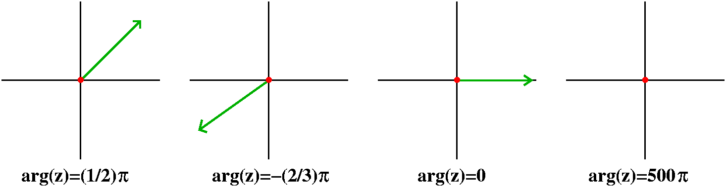
The specific A chosen in the text (so [-Π,Π) contains all of Arg's
values) is so that Arg will be continuous near points on the positive
real axis.
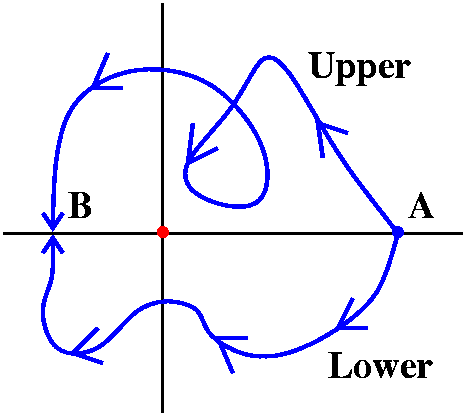
Suppose A is a point on the positive real axis. Then near A, Arg will
vary continuously. Points near A in the upper halfplane will have Arg
values near 0 and positive, and those near A in the lower halfplane
will have Arg values near 0 and negative. Suppose, though, we try to
move farther away. Look at the two parts to the right. On the Upper
curve, the values of Arg will increase (except around the loop!) and
especially as the Upper curve points near B (on the negative real
axis), they will increase to Π. What happens on the lower loop? There
the values of Arg will descrease, and as the points move (?) towards
B, the values of Arg will tend to -Π. So Arg is actually not
continuous at B. Depending on the direction of approach, there may be
a jump of + or –2Π in Arg's value. So:
Arg is not continuous at any negative real number, and at such
a number, Arg has a jump discontinuity of magnitude 2Π.
From log to Log
Again, for non-zero w, a solution of ez=w is called
log(w). If y=Arg(w), then the solution is called Log(w) (note
the capital letter!). The different formulas for log give what are
sometimes called branches of log. In this jargon, Log would
then be called the principal branch becuase it has the standard
real information, the most familiar, included in it.
The complex exponential function has many pleasant and some irritating
aspects. It is a bit difficult to draw a true graph of this
function. The domain points are in C which is
R2, as are the range points. Therefore the graph,
the pairs of points (z,ez) would be elements of
R4, and I don't know any neat ways of showing
four-dimensional graphs. (Many attempts of been made. For example, we
could sketch (x,y,u(x,y)) and change this standard graph of a surface
in R3 to the graph (x,y,v(x,y)) by some geometric
process. Or one could "draw" the graph of u(x,y) and put colors on the
graph according to the values of v(x,y). You can easily find these
methods and others on the web. I'll stick to more ordinary methods
here.
The most interesting aspect of the function which will be shown in its
mapping properties is that exp is 2Πi periodic. This means that exp
is infinite-to-1. Every non-aero complex number w has
infinitely many z's with exp(z0-w, and these are all separated by
2Πi.
|
I'll have a complex plane representing the domain to the left, and
then a range complex plane to the right. I'll try to sketch objects on
the left in the domain and then sketch the corresponding objects on
the right, objects which "correspond" under the exponential mapping.
|
|
One horizontal line
Consider the horizontal axis. We could image a bug moving on the axis
in the domain at uniform velocity, from left to right. Here y=0, and x
goes from –∞ to +∞. The image in the w-plane is
excos(0)+i exsin(0) which is
ex. Notice that this is a ray, a halfline, whose
image covers the positive x-axis. There is a further difference:
kinetic. The image of uniform motion is no
longer uniform motion. Near "–∞" the image bug moves very
slowly, and as the image goes from left to right along the positive
x-axis, the image bug moves ever faster, exponentially faster.
|
|
One vertical line
Now consider the vertical imaginary axis, where x=0, and a bug
crawling at uniform velocity from –∞ (in y) to +∞ (in
y). Now with x=0, the image is
e0cos(y)+i e0sin(y). So the image is the unit
circle, described in the positive (counterclockwise) fashion, with the
circle drawn at uniform velocity (1 radian per timestep).
|
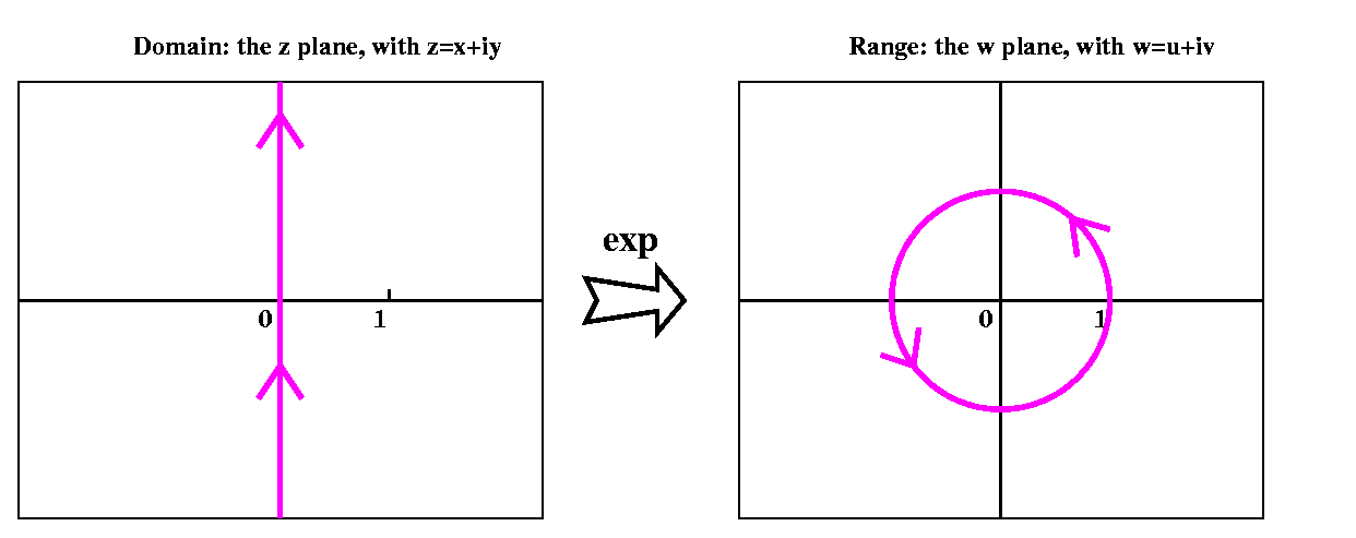
|
Other horizontal lines
If we look for the image of a horizontal line which is just slightly
above the x-axis, what will we get? Here we have
excos(y)+i exsin(y) with y a small
positive number. In fact, in terms of vectors, this is all positive
(ex) multiples of the unit vector [cos(y),sin(y)]. So the
image is again a halfline, a ray, emanating (originating?) from 0 at
angle y to the positive x-axis. You could imagine as the horizontal
lines go up or go down, the images will rotate around the origin.
|
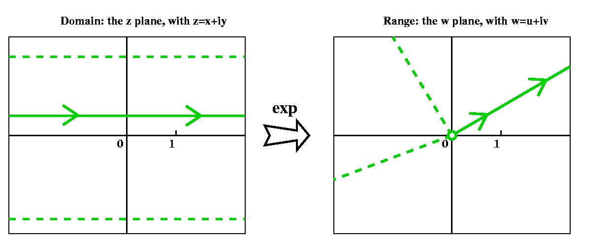
|
Other vertical lines
If we look for the image of a vertical line which is to the right of
the y-axis, what will we get? Here we have
excos(y)+i exsin(y) with x a positive
number. In fact, this describes a circle whose center is the origin,
and whose radius is ex, always a positive real number. You
could imagine as the vertical lines go left or right, the images will
all be circles centered at the origin of varying radii.
|
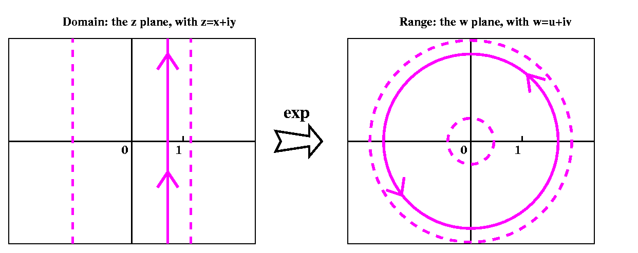
|
An oblique line
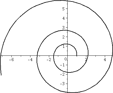 We even briefly considered an oblique line, and decided that its image
was a spiral. So if y=mx, say, with m>0, then the image under exp
of this is
exp(x+i my)=excos(my)+i exsin(my).
This is a spiral. somehow "interpolating" between a circle (the image
of a vertical line) and a ray from the origin (the image of a
horizontal line). To the right is a Maple
of part of one of those spirals with m=8.
We even briefly considered an oblique line, and decided that its image
was a spiral. So if y=mx, say, with m>0, then the image under exp
of this is
exp(x+i my)=excos(my)+i exsin(my).
This is a spiral. somehow "interpolating" between a circle (the image
of a vertical line) and a ray from the origin (the image of a
horizontal line). To the right is a Maple
of part of one of those spirals with m=8.
Although Maple has a complexplot command (part of the plots package) this is what I did to create
the picture shown. First, from y=8x I decided that I needed to
understand exp(x+8x i). So I computed:
exp(x+8x i)=exp(x)exp(8x i)=ex(cos(8x)+i sin(8x))=
excos(8x)+i exsin(8x))
and from this used the Maple
command
plot([exp(t)*cos(8*t),exp(t)*sin(8*t),t=-0.01..2],numpoints=100,thickness=2,color=black);
(I increased the default of numpoints
from 50 because I wanted a smoother curve.
Strips mapped by exp
We also saw how strips were mapped by exp. A horizontal strip which is
less than 2Π high will be mapped into a wedge of the plane, with
the corner of the wedge at 0. exp exactly matches the points in the
horizontal strip 1-to-1 with points in the wedge.
A vertical strip will always be mapped
onto an annular region, but this mapping is infinite-to-1.
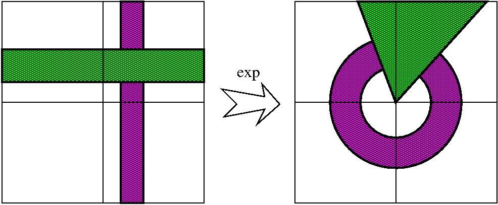
Finally, one last picture which attempts (poetically? qualitatively?)
to show you what exp does to the plane. We start on the left with an
R2. Then we pick it up and a hand, infinitely far to the
left (?), "squeezes" that side to a point. Then we expand this fan over
and over itself (?) infinitely many times and finally we project the
resulting bunch of knitted-together (?) discs onto another copy of
R2. This is the geometry of the exponential mapping on a
big-scale level.
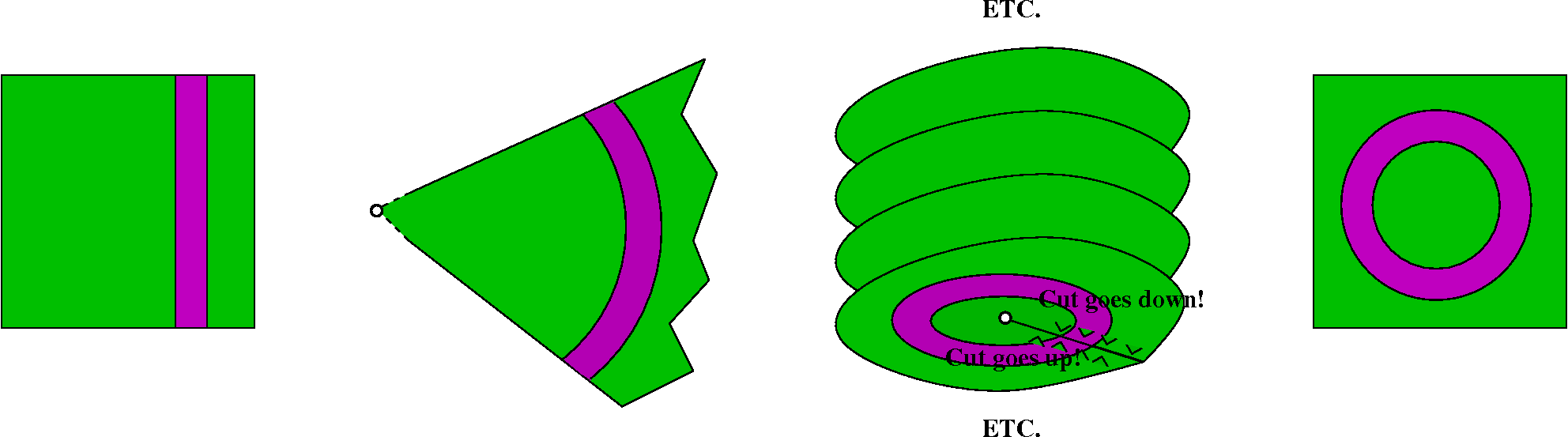
Some finer features which turn out to be very important in
applications are not at all clear in this presentation. For example,
curves in the left-hand, domain, plane are mapped to curves in the
right-hand, range, plane so that the angles of intersection of the
curves do not change! This is not obvious, and we will study these
angles in detail later.
Here, in italics, are notes from a previous instantiation of
this course describing the experiment with logs that I did, this time,
without student participants.
Three of the wonderful students in the class volunteered (always
better than the truth, which is closer to were dragooned) to
draw some pictures with me. I only show the results of three of the
students. I set up the exponential function mapping from a domain copy
of C to a range copy of C. Then I stood at the range
copy, with my chalk at w=1, which I also called HOME. I asked each of
the students to choose a value of log(1) different from 0. Since this
is a complex analysis course, there were certainly enough
distinct values to choose from. Each student could have their own
value of log(1). In my head I saw a sort of mechanical linkage reaching
backwards from my 1 to their choices of log(1). The linkage
would "automatically" respond to any changes of position in my
location by moving to nearby places whose value of exp would be where
my chalk moved to. Sigh. There's no pathology in this course:
things will be continuous, things will move nicely, etc. Much more
subtle problems will be met.
The first trip
Then I carefully and slowly (well, almost) moved my chalk from HOME in
a simple closed curve. The curve was made up of circular arcs centered
at the origin and pieces of rays which started at the origin. I used
these curves because last time we had previously computed how vertical
and horizontal lines in the domain were mapped. The inverse images of
my "trip" from HOME to HOME were carefully drawn. They were congruent,
because exp is 2Pii periodic. Each started from each student's
choice of log(1) and returned to that choice.
|
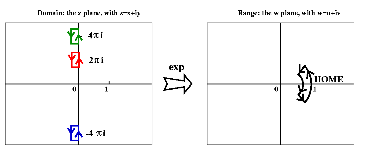
|
The second trip
Well, now I left HOME and traveled in a circle around 0, and returned
to HOME. The students attempted "follow" me in the domain of exp, and
there was some controversy. If we tried to make everything continuous,
then, even though my path in the range was a simple closed curve, each
student draw a path going from one choice of log(1) to another choice
of log(1). This is very, very mysterious.
I drew a few more paths in the range and mentioned what would happen
in the domain, and said we would need to explain all this is great
detail later. This is one of my goals in the course.
|
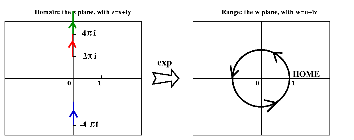
|
Linear mappings
We know (we have linear algebra knowledge) that a random linear
mapping from R2 to R2 is represented by a
matrix,
( a b )
( c d )
so that the pair, (x,y) in the domain, becomes
(ax+by,cx+dy) in the range. I may have this wrong, and maybe I should
be writing transposes of things, which is why I am not allowed to
teach linear algebra. So here is the interesting idea: which of these
mappings should be studied in a complex variables course? They are all
equally "nice" from the real-linear-algebraic point of view, but ...
The surprise, which will turn out to be profound, is that there is a
serious restriction. We want to study in this course only
linear mappings which occur as a result of multiplication by a complex
number. So if z=x+i y, and Q=α+i β, then we would
like to look at only mappings coming from z→Qz (complex
multiplication!). Now what happens algebraically? Look:
(x,y) corresponds to z=x+i y →
Qz=(αx–βy)+i (αy+βx) which corresponds
to (αx–βy,αy+βx)
This last vector is the result of using the 2-by-2 matrix
( α  –β )
( β   α )
So in this course we will look only at linear transformations which
have this rather peculiar restricted form: very weird.
| Wednesday,
January 27 | (Lecture #3) |
|---|
Today we study some nouns and maybe a few adjectives.
Nouns?
By "nouns" I mean here some of the standard terminology which is used
in "analysis" -- the grownup word for calculus and all of its
extensions. There will be a string of definitions, maybe punctuated by
some examples and some questions. The definitions are just to give us
enough common words so we can discuss usefully the phenomena (!) of
the course. I will not concentrate on the logical intricacy of
the definitions (we have several other courses doing that).
Dr(p)
The open disc
of radius r whose center is the complex number p. | Here p is
a complex number and r is a positive real number. Then
Dr(p) is the collection of complex numbers z with
|z-p|<r |
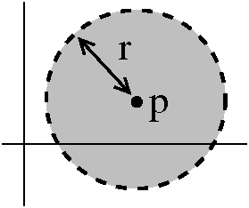 |
| An open set of complex
numbers |
Suppose U is a collection of complex numbers. Then U is
open if for every number p in U, there is some positive real
number r (which may depend on p!) so that Dr(p) is entirely
contained in U.
You've got to be able to put a disc inside U for every p in U.
|
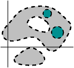 |
| Boundary point
|
The complex number q is a boundary point of a set W of complex
numbers if every disc of positive radius r centered at q,
Dr(q), contains at least one point in W and
at least one point not in W.
For the sets shown to the right, t is in U and is not a
boundary point of U, because the disc shown is entirely inside U and
has no points of V. The
point s is a boundary point of both V and U since
every disc of positive radius has points in V and points in U.
|
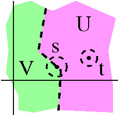 |
| Polygonal
curve |
A polygonal curve is a finite number of line segments
L0, L1, L2, ..., Ln, so
that the end of Lj is equal to the beginning of
Lj+1 for 0<j<n.
|
 |
| Connected open set |
An open set is connected if every pair of points in the set
can be joined by a polygonal line which is entirely inside the set.
Again, every pair of points must be joined by some polygonal
line totally inside U.
|
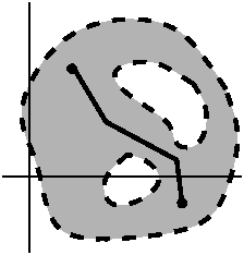
|
Now let us consider some examples.
| The set & its owners | Is it open? | If it is
open, is it
connected? | Describe all the boundary points of the
set | Picture of the set |
|---|
D1(0)
This is the open unit disc: those z's with |z|<1.
Owned by: Mr. Glass & Mr. Breuer.
| The set is open (needs Δ≤ to check this: for a
disc centered at p use as
radius 1–|p|, or look at
the picture). | Yes, connected. Any two points in the disc have
a line segment connecting them which lies entirely inside the
disc. | The boundary points satisfy |z|=1. Any disc of positive
radius centered at such a point has points both in the set and not in
the set. |

|
| A set is convex if, whenever two points are
in the set, the line segment containing the points is entirely within
the set. So a circle (the boundary of a disc!) is not convex,
but a line segment itself is convex. The unit disc is an example of a
convex open set, and convex open sets are always connected (the
polygonal curve is just one line segment!)
|
z's with |z|≤1
Sometimes called the
closed unit disc.
Owned by: Ms. Janiszewski & Mr. Sirisky. | This is not
open. Consider the point p=1, in this set. Every disc of positive
radius centered at 1 has points on the real axis to the right of 1,
and therefore such a disc is not contained in the set. | Does
not apply. |
Again, the boundary is |z|=1. The verification is the same as the
previous example. |
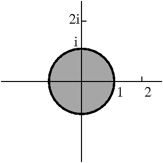
|
z's with 1<|z|<2
This is
called an annulus (the region between two concentric
circles).
Owned by: Mr. Russo &
Mr. Zhang. | This is an open set. | Yes, this open set is connected. However, the
connecting polygonal line may need more than 1 segment to go from one
point to another. (I think it may need as many as 3 segments -- can
you think of a connected open set which might need more?)
|
The boundary has two "pieces": one of all the z's satisfying
|z|=1 and the other of z's satisfying |z|=2. |
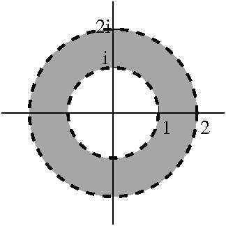
|
z's with 1<|Re(z)|<2
Owned
by: Ms. Addabbo & Mr. Laflotte. | This is an open set. If p is in the right-hand strip,
say, then
1<Re(p)<2, then a disc of radius
min(2–Re(p),Re(p)-1) will be inside the strip. Dics can be
created for points in the left-hand strip similarly.
strip is |
No. This set is not connected. For if it were, then the
function Re(z) would have to be continuous when restricted to the
polygonal line. If we try to "connect" –1.5 and 1.5, the
function (by the one-variable Intermediate Value Theorem) would be 0
somewhere on the polygonal line, and no point in the set can have
Re(z)=0. The polygonal line cannot be contained in the set. |
The boundary is 4 straight lines :Re(z)=+/–1 and Re(z)=+/–2. |
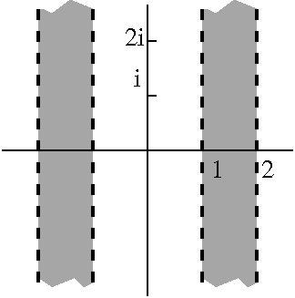
|
z's where
z3/(z2+3z+2) is defined
Owned
by: Mr. Dyson & Mr. Yeager. | We'd better throw away z's where
z2+3z+2=0. We can factor polynomials in a field to
get roots, so z2+3z+2=(z+2)(z+1) indicates that –1
and –2 should be thrown out. The resulting set is open (if p is
in it, take a radius of min(|p–(–1)|,|p–(–2)|)
to get a disc entirely in the set).
| This set is connected. Draw some vertical and horizontal
lines through any pair of points in the set, and once they are away
from the real axis, they can be "connected". |
The boundary consists exactly of the two points –1 and
–2, because a disc around one of those points will aways contain
points in the set and also will contain the center of the set, which
is not in the set. |
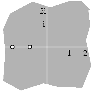
|
Associated question
Is C "minus" a finite number of points open and connected? (That is,
everything except those finitely many complex numbers.) What are the boundary
points of this set?
Answer
Yes, such a set is open and connected, and the boundary
is just the finite number of points which were thrown out. Therefore,
for example, the domain of a rational function (quotient of
polynomials) will be a connected open set. |
All z's with 1≤Re(z)<2 and
1<Im(z)<2
Owned by: Mr. Leung & Mr. Mohamed. | This is
not as open set. Just look at the point z=1+1.5i. No disc of
positive radius centered at 1+1.5i is entirely in the set. |
Does not apply. |
The boundary is 4 line segments: Re(z)=1 and 1≤Im(z)≤2,
Re(z)=2 and 1≤Im(z)≤2,
1≤Re(z)≤2 and Im(z)=1, and
1≤Re(z)≤2 and Im(z)=2.
|
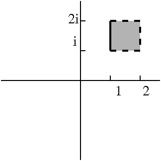
|
Comments on strategies
To verify in detail that a set is open, you must show that if z is
any point in the set, then there is at least one positive
radius r so that Dr(z) is in the set.
To verify in detail that a set is not open, you must shown that
there is at least one z in the set so that if r is any positive
radius, then Dr(z) always has points not in the set (it is
not contained totally in the set).
So the logic is a little twisty: the quantifying phrases "all" and
"there is at least one" play a part in both verifications. Such
logical intricacies will not be a large part of this course -- we have
other sorts of intricacies!
Question α for Mr. Marcus
& Mr. Ronan:
- Suppose an open set U has the property that for all p in U,
D5(p) is contained in U. What is U?
Answer First a little bit of logic: the empty set (the set with
no complex numbers in it at all!) does satisfy this specification,
because of the vacuous nature (no requirement!) of the hypothesis. The
usual symbol for this set is ∅. But
what if U is not empty? Suppose p is in the set and q is some
other complex number. Consider the line segment
joining p and q. "Walk" along that line segment with steps of length
4, say (the key is that 4<5 here!). All of the points in each
segment, starting at p, must be in U because the discs successively
are all in U. So eventually we see that q is in set also. So actually,
U must be all of C!
- Suppose an open set U has the property that for all p in U,
D1/17(p) is contained in U. What is U?
Answer U will either be the empty set or all of C. The
reasoning is sort of the same, using steps of length less than 1/17.
- Suppose an open set U and there is a positive real number r so
that for all p in U, Dr(p) is contained in
U. What is U?
Answer Again, U is either empty or all of C.
Comment What this question shows is that in all but the
simplest circumstances, the radius used in the definition of "open
set" must vary with the point chosen as center.
For logical sophisticates (?), this shows that interchanging the
universal and existential quantifiers phrases ("For all ... there exists") in
the defintion of open set yields something that's only satisfied by
two examples!
 Question β for Mr. Cantave
& Mr. Khor:
Question β for Mr. Cantave
& Mr. Khor:
Must the intersection of two connected open sets be connected? If
the answer is yes, briefly explain why. If the answer is no, give some
useful examples showing what can happen.
Answer The intersection of two open connected sets may be
connected. For example, the intersection of two open discs is an open
connected set. But the intersection may not be connected, for
example, consider the picture to right. The two "blobs" pictured are
open, and their intersection has two pieces. This somewhat simple
picture will turn out to have important computational consequences.
Question γ for Mr. Sherman
& Ms. Koshibe:
(Many  's not shown!)
 |
- Suppose S is the sequence of numbers 1, 1/2, 1/3, 1/4, 1/5, .... (this
is an infinite collection of numbers). Suppose W is all
complex numbers except those in S (the complement of S). Is W
open? What are the boundary points of W?
Answer Well, the problem is at 0. 0 is in the set W, but every
disc of positive radius centered at 0 will have some of the 1/n's in
it. So W is not open. The boundary points of W are all the
points of S (just as in the simpler example with two points removed in
the table able) and also the point 0, since there are also
points of W in any disc of positive radius.
(Many 's not shown!)
 |
-
Suppose T is the following set: the sequence of numbers 1, 1/2, 1/3,
1/4, 1/5, .... (this is an infinite collection of numbers)
and also the number 0. Suppose Q is all complex numbers except
those in T (the complement of T). Is Q open? What are the
boundary points of Q?
Answer We seem to have removed the problem! If a point is far
away from the sequence T and is not 0, then there is certainly a disc
entirely contained in Q with center at that point. So the set Q
is open. Its collection of boundary points remains the same as
in the previous example: all the points of S and also the point 0.
Notice the examples just presented each involve taking an infinite
number of points out of C and then inspecting the result. If we take
only finitely many points away, then (see the example above analyzed
by Mr. Dyson & Mr. Yeager) the result is always open and
connected. Here we see that the "geometry" of the infinite number of
points allows a more varied result. The set might or might not
be open. I can tell you (this is not obvious!) that if the set is
open, then it must be a connected open set.
|
A closed set is one which contains its boundary.
|
Here is a
theorem on page 25 of the text:
Theorem A set U is open if and only if if contains no point of
its boundary. A set K is closed if and only if its complement (those
complex numbers which are not in K!) is open.
The proof is on page 25, and I will sometimes use this result but I
don't want to go through the proof which is logical tail-chasing. (I
am not declaring that the proof is silly, just that it is not in the
mainstream of the concerns of this course!) If you like this sort of
reasoning, you can take Math 311 or Math 441.
|
Which of the sets we
have investigated are closed? Which are neither open nor closed?
Answers
- The open unit disc, the set of Mr. Glass & Mr. Breuer, is open and is not closed.
- The closed unit disc, the set of Ms. Janiszewski & Mr. Sirisky, is closed and is not
open.
- The annulus, the set of Mr. Russo &
Mr. Zhang, is open and is not closed.
- The double infinite strips, the set of Ms. Addabbo & Mr. Laflotte, is open and is
not closed.
- The "doubly punctured plane", the set of Mr. Dyson & Mr. Yeager, is open and is
not closed.
- The weird square, the set of Mr. Leung & Mr. Mohamed, is not open and is
not closed. (Nomination for the worst math terminology in
English and in the other languages I know: "open" and "closed": I know
sets which are both [below] and I know sets which are neither!)
- In question α, analyzed by Mr. Marcus
& Mr. Ronan, the empty set and the whole complex
plane are both open and closed.
- In question β, analyzed by Mr. Cantave
& Mr. Khor, I can tell you that the intersection of
two open sets will always be open (but the intersection of infinitely
many may not be!). The intersection of two closed sets is
always closed, and, in fact, the intersection of any number of closed
sets is closed. If you know de Morgan's laws (how to manipulate sets)
then you can deduce what happens to unions of these sets. We will not
need such results here.
- In question γ, analyzed by Mr. Sherman & Ms. Koshibe, the set W is not open and
it is
not closed. The set Q is open and is not closed.
| Monday,
January 25 | (Lecture #2) |
|---|
There are two topics today: the Triangle Inequality and de Moivre's
Theorem. Let's start.
Simple ? stuff
I'll repeat a few geometric definitions, stated in "complex
language". If z=a+bi, then a=Re(z), the real part of z, and b=Im(z),
the imaginary part of z. Also, we know some polar language:
z=r(cos(θ)+i sin(θ)) where we really know θ
only up to a multiple of 2Π and
|z|=sqrt(a2+b2). (There is a unique value
of arg(z) in any half-open interval of length 2Π such as [0,2Π)
or (-Π,Π] but different situations lead to different choices!) If
z=a–bi, the
complex conjugate of z, then zz=a2+b2
so that |z|2=zz. Please also note that if
z=r(cos(θ)+i sin(θ)) then z=r(cos(θ)–i sin(θ))=r(cos(–θ)+i sin(–θ)),
and therefore the modulus of z, |z|, is the same as |z|
and the argument of (or, one argument of!) z is
–arg(z). We showed last time that, with multiplication, the
modulus multiplies and the arguments add. Therefore |z||z|=|z| |z|=|z|2
and arg(|z|2) is arg(z)+arg(z)=arg(z)–arg(z)=0, so
that |z|2 is real and non-negative (this is
reassuring!). Therefore |z|2=z z. And notice that
|zw|2, which must be (zw)zw, is also equal to
|z|2 |w|2=zzww. Therefore zw=z·w.
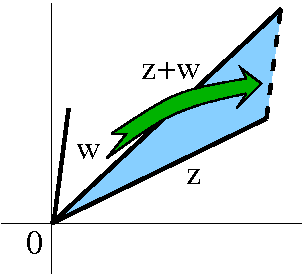 The triangle inequality
Much of this course will be devoted to getting precise and elaborate
formulas for complicated things. The most amusing aspect of this
endeavor is that it will depend on getting very sloppy
estimates of fairly simple things. The basic sloppy estimate for
most of analysis is the triangle inequality:
|z+w|≤|z|+|w|
Let's try to understand this inequality. First, some geometric
insight: complex number addition is just like 2-dimensional vector
addition, so if z and w are modeled by vectors based at the origin in
R2, then a picture we could consider is what's shown to the
right. To create z+w we move a copy of w to start at the "end" of
z. Then the triangle inequality states that the z+w side is
overestimated by the sum of the other two sides. This could be an
equality, of course, if the directions of z and w coincide.
It is almost always useful to understand things in more than one
way. Let's try to verify the triangle inequality algebraically. |z+w|
has a square root which I will try to avoid, so I'll begin with its
square: |z+w|2=(z+w)(z+w). But z+w is the same as z+w (check this either
geometrically by flipping z+w or algebraically by changing the sign of
the second coordinate in the two dimensional vectors). Let's try
again:
|z+w|2=(z+w)(z+w)=(z+w)(z+w)=zz+zw+wz+zw=|z|2+|w|2+wz+zw.
I will admit that one of the reasons for going through this
verification is so that you see some of the algebraic tricks we will
be using during most of the course. I need to analyze zw+wz. Well, we do know already
that Q·P=Q·P. Another useful fact is
conjugating a complex number twice gets back the original number
(bar-bar is the identity). You can see this geometrically by flipping
twice across the x-axis, or algebraically by – · –=+.
The "cross-term" is the sum of zw and its complex conjugate. But:
Re(P)={1/2}(P+P} and Im(P)={1/2i}(P–P).
Therefore zw+wz is actually 2Re(zw). But:
Re(P)≤|Re(P)|≤|P| and Im(P)≤|Im(P)|≤|P|
So:
|z+w|2=|z|2+|w|2+wz+zw≤
|z|2+|w|2+2Re(zw)≤
|z|2+|w|2+2|z|·|w|=(|z|+|w|)2.
Taking square root (just square root of non-negative reals!) gets us
the triangle inequality.
Some numerical estimates
Suppose we have P(z)=z5–(2+i)z3+9. How big can
|P(z)| be on the circle of radius 2 centered at 0 (that is, where
|z|=2)? Here we go:
|P(z)|=|z5–(2+i)z3+9|≤
|z5|+|–(2+i)z3|+|9|=|z|5+|2+i|·|z|3|+9=25+sqrt(5)23+9=41+8sqrt(5).
Can we get an underestimate? Here is an important variant of the
triangle inequality:
|z|–|w|≤|z+w|
Why is this true? It is the same as |z|≤|z+w|+|w| and remember that
z=z+w–w so that using the original
triangle inequality, we have
|w|≤|z+w|+|–w|=|z+w|+|–1| |w|=|z+w|+|w|.
Of course, while the inequality |z|–|w|≤|z+w| is always true
it may sometimes have very little information. For example, if z=1 and
w=5, then we get –4≤6: rather silly. We want |z| to be larger than
|w| otherwise the left-hand side is negative, and we learn nothing. I
prefer, in fact, to think of this "reverse" inequality in the
following way:
|BIG|–|LITTLE|≤|BIG+LITTLE|
Now consider |P(z)|=|z5–(2+i)z3+9| when
|z|=2. Here I will take BIG to be z5 because then
|z5|=32. I will take LITTLE to be –(2+i)z3+9
because then I can overestimate
|LITTLE|=|–(2+i)z3+9|≤sqrt(5)|z|3+9
which is 8sqrt(5)+9 when |z|=2 (that is less than 27 -- you can check
this!). Then |BIG|–|LITTLE|≤|BIG+LITTLE| becomes
32–(8sqrt(5)+9)≤|P(z)| or 23–8sqrt(5)≤|P(z)| if
|z|=2.
| We can now conclude that the values of P(z) for |z|=2
must lie inside an annulus centered at 0. That is, if |z|=2 and
w=P(z), then r≤|P(z)|≤R where R=41+8sqrt(5)≈58.9 and
r=23–8sqrt(5)≈5.1. The picture shown is not true to
scale. The r and R and 2 are not in correct proportion. Notice I am
not asserting that every w inside that annulus is a value of
P(z) for |z|=2. That is false. In fact, the image of the circle is a
curve inside the annulus. We'll see that the curve in fact twists 5
times around the center of the annulus. | 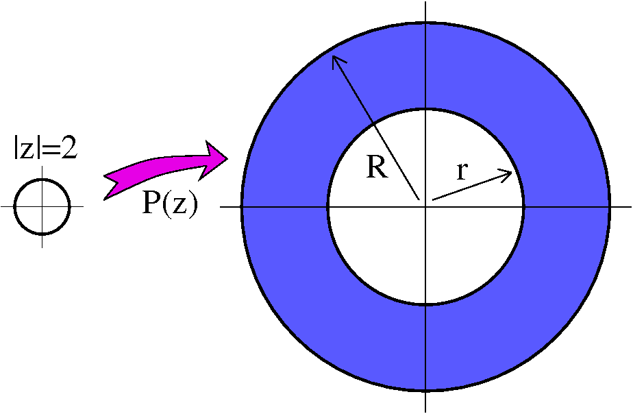 |
|
I'll use this background color for material I didn't do
in class because it wasn't convenient (some computations or pictures,
for example!) or because I didn't have time, but which you might find
interesting.
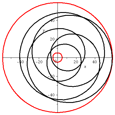
What does it really look like?
Here is a Maple picture of the image of
|z|=2 under the mapping z→P(z): the black curve. The red circles
are circles of radius 5.1 and 58.9 centered at the origin. The curve
is inside the predicted annular region. It is certainly not always
true that the methods outlined always will give such a tight fit. I
think we are just lucky here because P(z) is fairly simple!
|
|
Quick, let's try again: consider Q(z)=z2–7z. Then
|Q(z)|=|z2+7z|≤|z2|+|7z|=|z|2+7|z|
and this is at most 18 if |z|=2. What about an underestimate? Some
thought will show that we get information in this case if BIG is 7z
(which has modulus 14) and LITTLE is z2 (modulus 4). So
14–4=10 is an underestimate. And therefore 10≤|Q(z)|≤18 if
|z|=2.
We can compound the achievement (if we call it that!). We could consider the rational function R(z)=P(z)/Q(z)=z5–(2+i)z3+9
------------
z2–7z
I bet that the values of |R(z)| for |z|=2 are between
{23–8sqrt(5)}/18 (about 2.8) and
{41+8sqrt(5)}/10 (about 5.9).
- To get an underestimate of a quotient, take the min
of the top and the max of the bottom.
- To get an overestimate of a quotient, take the max
of the top and the min of the bottom.
Some algebra
We know that if z=r(cos(θ)+i sin(θ)) and
z=s(cos(λ)+i sin(λ)), then
zw=rs(cos(θ+λ)+i sin(θ+λ)). Careful use
of this formula will allow use to "explicit" solutions to certain
rather simple polynomial equations. Later in this course, we'll see
that all polynomial equations have solutions, although there won't be
nice formulas for them.
Let's try to solve z3=5i. The modulus of 5i is 5 and its
argument (or, better, an argument) is Π/2. If
z=r(cos(θ)+i sin(θ)) then
z3=r3(cos(3θ)+i sin(3θ)). When
will this be 5i? Certainly the modulus information is carried by
r3, so that if z is a cube root of 5i, then
r3=5 and r must be 51/3. By 51/3 I
mean precisely the unique positive real number whose cube is
5. (That's about 1.71.) What about the argument? I know that
cos(3θ)+i sin(3θ))=0+1i, which means that θ is
some number with cos(3θ)=0 and sin(3θ)=1. Let's think:
3θ should be Π/2 (plus possibly some
multiple of 2Π) or 3Π/2 (plus possibly
some multiple of 2Π).
If 3θ is the first alternative, then
θ must be
Π/6 or
Π/6 + 2Π/3 or
Π/6 + 4Π/3.
If 3θ is the second alternative, then
Π/2 or
Π/2 + 2Π/3 or
Π/2 + 4Π/3.
But we also need sin(3θ)=1. Since sin(3{Π6})=1 and
sin(3{Π2})=–1, the solutions are only those resulting
from the first alternative. We have deduced that solutions of
z3=5i include these numbers:
51/3(cos(Π/6)+i sin(Π/6))
51/3(cos(Π/6+2Π/3)+i sin(Π/6+2Π/3))
51/3(cos(Π/6+4Π/3)+i sin(Π/6+4Π/3))
We can even write these in rectangular form since I happen to know
that sin(Π/6)=1/2 and cos(Π/6)=sqrt(3)/2. The solutions we
have found can also be written as:
51/3(sqrt(3)/2)+51/3(1/2)i;
–51/3(1/2)+51/3(sqrt(3)/2)i;
–51/3(sqrt(3)/2)–51/3(1/2)i
Some questions: are there any other solutions to the equation
z3=5i? What is the significance (if any!) of these
solutions?
Let me answer the first question. If we are working in a field,
then most of high school algebra carries over (anything relying on
addition, multiplication, subtraction, division). In high school we
saw that if P(UNKNOWN) is a polynomianl,
and if α is a root (so P(α)=0) then P(UNKNOWN)=(UNKNOWN–α)Q(UNKNOWN) where Q(UNKNOWN) is a polynomial of degree one less
than the degree of P(UNKNOWN). 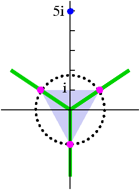 This
leads to the realization that a polynomial can have only as many
distinct roots as its degree. Since z3–5i has degree 3, it
can have only 3 distinct roots, and we've found 3 distinct roots. So
there aren't any more.
This
leads to the realization that a polynomial can have only as many
distinct roots as its degree. Since z3–5i has degree 3, it
can have only 3 distinct roots, and we've found 3 distinct roots. So
there aren't any more.
The picture is incredibly full of information. It shows 5i, and then
the 3 cube roots are displayed. Notice please that they form the vertices
of an equilateral triangle whose center is at the origin, and whose
radius is 51/3. The angular "offset" from the positive
x-axis of a vertex of this equilateral triangle is one-third of the
argument of 6i.
I hope that this discussion will persuade you to accept my declaration
(!) of all solutions of the equation zn=A where A is
any complex number (well, if A=0, then the solution(s) are all
0, so maybe I'd better write "A is any non-zero complex
number") and n is a positive integer.
The geometry of z when zn=A if A≠0
Here is how to display the n solutions of the equation zn=A
for a non-zero A. First, draw a circle of radius |A|1/n (a
unique positive real number). Now draw an equilateral polygon with n
sides inscribed in this circle. Here inscribed means that the
corners or vertices of the polygon are on the circle and the sides are
all inside the circle. For precision, put one of the vertices on the
positive real axies. Then the polygon should be offset or
rotated in the positive, counterclockwise direction by the
argument of A divided by n. The vertices of the resulting object are
the distinct nth complex roots of A.
Examples
Probably the most important collection of examples occur when A is
just 1. The roots are called the
nth roots of unity. Below is a picture of these
roots for n running from 2 to 6. Since arg(1)=0, the rotational offset
is 0, and one vertex of the regular polygon determined by the roots
will always be 1.
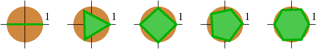
O.k.: let me try to do more specific computation in one last example:
z4=–1+i. Here 1+i has modulus sqrt(2) and (one value of)
argument 3&Pi/4. So what are the fourth roots of 1+i? Since
|1+i|=sqrt(2), I know that the fourth roots all must like on the
circle of radius 21/8 centered at the origin. What about
their arguments? Well, they will be "separated" by 2Π/4 and
will "start" at (3Π/4)/4 which is 3Π/16. So here are the
4th roots of 1+i:
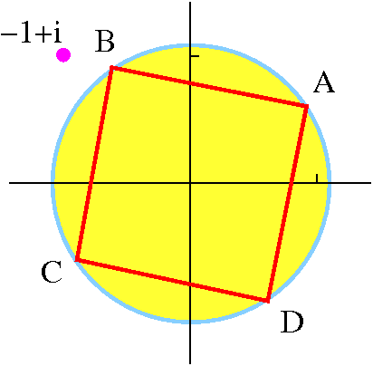 A=21/8(cos(3Π/16)+i sin(3Π/16));
B=21/8(cos(11Π/16)+i sin(11Π/16));
C=21/8(cos(19Π/16)+i sin(19Π/16));
D=21/8(cos(27Π/16)+i sin(27Π/16)).
A=21/8(cos(3Π/16)+i sin(3Π/16));
B=21/8(cos(11Π/16)+i sin(11Π/16));
C=21/8(cos(19Π/16)+i sin(19Π/16));
D=21/8(cos(27Π/16)+i sin(27Π/16)).
In the picture to the right, the circle is supposed to have radius
21/8.
Comments and objections
I didn't really compute them, did I? I think I did, but what if
you wanted a rectangular description of them? Let's try the first one
and try to get some numbers for cos(3Π/16)+i sin(3Π/16). I
know cos(3Π/4): that's –1/sqrt(2). But I also know that
cos(2w)=2(cos(w))2–1. So (taking w=3Π/8)
–1/sqrt(2)=2(cos(3Π/8))2–1. This has roots
(1/2)sqrt(2–sqrt(2)) and –(1/2)sqrt(2–sqrt(2)). I'll take the positive
root since cos(3Π/8) is positive (0<3Π/8<&Pi/2). Then
another half angle computation leaves me the choice between
(1/2)sqrt(2+sqrt(2–sqrt(2))) and –(1/2)sqrt(2+sqrt(2–sqrt(2))) so I
choose (1/2)sqrt(2+sqrt(2–sqrt(2))), and this is cos(3Π/16). Then
sin(3Π/16) turns out to be (1/2)sqrt(2–sqrt(2–sqrt(2))). The first
(?) root in the list above is therefore
2–7/8sqrt(2+sqrt(2–sqrt(2)))+
2–7/8sqrt(2–sqrt(2–sqrt(2)))i. Maple tells me that the fourth power of this
is indeed –1+i. (Wow! Of course this is rather special reasoning,
using crazy identities which in fact are best understood with complex
analysis -- see de Moivre's result which follows.)
Dynamics
A more intricate "exercise" is to imagine what happens if I take
z=–1+i and start to move it. If I move it radially (slightly in
or out) the corresponding fourth roots will vary also, of course. They
will move in or out, always staying in a square centered at 0. What if
I move z counterclockwise? In that case, the fourth roots will also
move counterclockwise, but their rotational velocity will be
one-fourth that of z. And if we move z fully around the origin,
returning to 1+i, the vertices of the square will each be shifted
cyclically, A to B, B to C, C to D, and D to A.
De Moivre's Theorem
This result is a special case of the reasoning we've just
discussed. Here it is:
(cos(θ)+i sin(θ))n=cos(nθ)+i sin(nθ)
People have used this result to do all sorts of wonderful
computations. For example, let's try n=3 and "expand" the left-hand
side (binomial coefficients!):
(cos(θ)+i sin(θ))3
=1cos(θ)3+3cos(θ)2{i sin(θ)}1+3cos(θ)1{i sin(θ)}2+1{i sin(θ)}3
=cos(θ)3+i 3cos(θ)2sin(θ)1–3cos(θ)1sin(θ)2–i sin(θ)3
This is supposed to be the same as cos(3θ)+i sin(3θ). We can compare the real and imaginary parts of both "sides" and get:
cos(3θ)=cos(θ)3–3cos(θ)sin(θ)2 (the real part)
sin(3θ)=3cos(θ)2sin(θ)–sin(θ)3
(the imaginary part)
Maybe these triple angle formulas are not immediately obvious!
Who he?
Abraham de Moivre was born in France (1667) and died in England
(1754). Here
is a neat short biography, which declares
De Moivre is also remembered for his formula for (cos x + i sin
x)n which took trigonometry into analysis, and was
important in the early development of the theory of complex
numbers. It appears in this form in a paper which de Moivre published
in 1722, but a closely related formula had appeared in an earlier
paper which de Moivre published in 1707.
De Moivre studied Newton's Principia thoroughly. Another
reference states
Eventually de Moivre become so knowledgeable
about the material that Newton would refer questions to him saying,
"Go to Mr. de Moivre; he knows these things better than I do."
That is quite a recommendation! De Moivre lived in poverty for most of
his adult life. In the first part of his life, he experienced
religious prejudice in France and then later, prejudice against
immigrants in England. Human beings are both wonderful and consistent,
and are sometimes not wonderful and still consistent.
|
| Wednesday,
January 20 | (Lecture #1) |
|---|
The information sheet was distributed,
so the students are now known.
Here are some problems which the techniques of this course can
investigate or solve or compute efficiently.
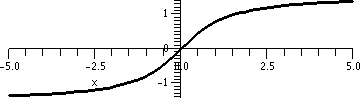 The function arctan(x) has a graph which is very nice, a smooth
strictly increasing curve through the origin. Also, we know from calc
2 that the Taylor series of arctan centered at the origin is ∑n=0∞(–1)nx2n+1/(2n+1). The radius of
convergence of this series is 1. What the heck goes wrong when
x→1– (or maybe x→–1+)? Is there some
invisible flaw in the function or tiny "kink" in the graph which
causes a problem? What is happening?
The function arctan(x) has a graph which is very nice, a smooth
strictly increasing curve through the origin. Also, we know from calc
2 that the Taylor series of arctan centered at the origin is ∑n=0∞(–1)nx2n+1/(2n+1). The radius of
convergence of this series is 1. What the heck goes wrong when
x→1– (or maybe x→–1+)? Is there some
invisible flaw in the function or tiny "kink" in the graph which
causes a problem? What is happening?
- There are many techniques for solving differential equations, and
we have several courses devoted to these techniques. One method is to
transform the equation using the Laplace transform or the
Fourier transform, and then analyze the result. Part of the resulting
computational "baggage" is computing specific definite integrals. For
example, the following improper definite integral,
∫–∞∞[cos(mx)/(1+x2)]dx
(here m is an arbitrary
real parameter) comes up when computing Fourier transforms. The
definite integral converges because the top is between –1 and +1, and
the bottom, which is never 0, decays like 1/|x|2 when
|x|→∞. In practice the exact
value of this integral is needed. Most standard computer algebra
systems (surely Maple or Mathematica) can give a (remarkably!) simple
answer. How do they do it? If you think about some of the standard
"tricks" to compute integrals (integration by parts? substitution?)
you would probably realize that they are inappropriate in this
case. How do these programs compute the integral? How difficult is it
and can this computation be done "by hand"?
- One of the very classical models of many physical situations
involves the following partial differential equation: Δh=∂2h/∂x2+∂2h/∂y2=0. One phenomenon (among many) which this
models is "steady state heat flow in an isotropic medium": that is,
say, a thin metal plate where a boundary temperature is prescribed and
the temperature inside the plate doesn't change with time. A solution
of the differential equation is called a harmonic function. The
combination of the differential equation (Laplace's equation) and the
boundary condition is called the Dirichlet problem. It turns
out that, under fairly mild assumptions, there is a unique solution to
the Dirichlet problem. Maybe this is not obvious, but the way to
convince yourself that this is true is to start heating or cooling the
edge of a plate, and just let the heat "propagate" until an
equilibrium is reached. The same partial differential equation also
models other phenomena. O.k.: there is a solution. But how can
we actually find or compute the solution?
 For example, we
could "prescribe" the boundary temperature on the unit disc. One
(seeming!) very simple boundary distribution might be temperature=1 on
the upper half of the boundary, and temperature=0 on the lower half of
the boundary. If then we want an equilibrium temperature distribution
on the inside of a disc-shaped plate, my guess is that the inside
temperature will be between 0 and 1 (hey, if a point inside had
temperature 150, I bet it would leak lots of heat to the boundary). I
also think that the symmetry of the boundary temperature would result
in symmetric isothermal curves inside the disc. O.k.: I can do this
much by "pure thought", but how can I now actually compute the inside
temperature? What are those curves?
For example, we
could "prescribe" the boundary temperature on the unit disc. One
(seeming!) very simple boundary distribution might be temperature=1 on
the upper half of the boundary, and temperature=0 on the lower half of
the boundary. If then we want an equilibrium temperature distribution
on the inside of a disc-shaped plate, my guess is that the inside
temperature will be between 0 and 1 (hey, if a point inside had
temperature 150, I bet it would leak lots of heat to the boundary). I
also think that the symmetry of the boundary temperature would result
in symmetric isothermal curves inside the disc. O.k.: I can do this
much by "pure thought", but how can I now actually compute the inside
temperature? What are those curves?
There are a number of ways of investigating all three of these
situations, because they are important problems and many clever people
have looked at them. But most knowledgeable people would agree that
first way to consider the problems is to use "calculus with complex
numbers". And all three of these problems, which I admit I selected
for their seeming dissonance, are closely related. They can all be
very profitably understood using this complex analysis.
Just as in real calculus the variable is usually called x, in complex
analysis we call "the" variable is usually called z. And, just to
quiet speculation, the following equation is true:
 d
---(z5)=5z4
 dz
The elementary computational algorithms will all be unchanged: that's
easy. What turns out to be significant is what d/dz means. And
the results of that consideration make complex analysis in some
fundamental way much easier then real analysis but also very
different.
Introducing the main characters
The plane is a wonderful geometric object, and it can be thought about
in many different ways. Let me consider three of them.
- Two dimensional vectors: forces or velocities or ... So these
are arrows with a head and a tail. They are directed line segments and
the length is the magnitude, etc. They can be added by putting head to
tail, etc. So then every vector can be written as a sum of i
and j and ...
- R2: by this I mean the collection of all ordered pairs
(a,b), with a and b real numbers. We meet this formulation (hey: the
two-dimensional real vector space: formidable language!) for
example in linear algebra, where we learn to manipulate vectors
(actually in any dimension) using row reduction. We can multiply
vectors by scalars, add them, etc.
- The plane is also C, the complex numbers. Here I think of
a+bi (with a and b real) as a number, and I will assume that
i2=–1. Then I will try to follow my nose (?) and compute
with these things.
All three of these labelings really will refer to the same geometric
object, the plane. I can switch my point of view from one to the
other, whatever is convenient. So the vector ai+bj will
be the same as the ordered pair (a,b) will be the same as the complex
number a+bi.
What's a field?
To me, all of linear algebra is one algorithm plus lots of
definitions. Of course, this is a simplification, but not a huge
one. The algorithm has various names: I usually think of it as row
reduction. The definitions help us understand how to cope with the
information going in and out of the algorithm. To "run" row reduction,
we need to be able to add and multiply and to subtract and divide and
... Well, here are the organizing principles which seem to be
necessary.
Addition Addition is commutative and associative; there is an
additive identity and there are additive inverses.
Commutative means that the order of
addition doesn't matter: 3+7=7+3. Associative means that the
grouping doesn't matter: 3+(7+4)=(3+7)+4. The additive identity
means there is a number 0 so that 7+0=7 (for "all values of 7"). And
of course additive inverse means that there is a number –7 so
that 7+(–7)=0.
Multiplication Multiplication is commutative and associative;
there is an multiplicative identity and (for non-zero numbers!) there
are multiplicative inverses.
The words have meanings similar to what they mean for
addition. The only interesting variation is that 0 can't have a
multiplicative inverse ("You can't divide by 0.") because people
learned this was necessary to avoid some serious logical and
computational problems.
Distributivity (linking + and x) a(b+c)=ab+ac.
These "rules" are all that is necessary to do a very wide variety
of computation.
A very tiny field
0 (the additive identity) and 1 (the multiplicative identity) had
better be different. But just with those two numbers there is
enough to do arithmetic. What follows are tables defining addition and
multiplication. Certainly a century ago this was merely a mathematical
curiosity.
  + | 0 | 1      + | 0 | 1
 -----------    -----------
  0 | 0 | 1      0 | 0 | 0
 -----------    -----------
  1 | 1 | 0      1 | 0 | 1
Now we recognize that the tables in fact are vital to understanding Boolean
expressions (true/false) and the linear algebra algorithm is very useful
in analyzing complicated "statements". This field is called Z2.
I want to consider more natural (?) fields.
The field we grew up with
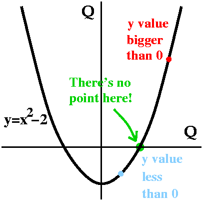 I want to count: 1, 2, 3, 4, 5, .... and divide up pies (half a pie or
a quarter of a pie for me, and a tenth of a pie for you). So we are
led to the rational numbers, Q, a very natural field. I like this
field. With patience, I can even compute moderately efficiently with
it. However, there is something wrong with it: a lack of
completeness which is upsetting to our intuition.
I want to count: 1, 2, 3, 4, 5, .... and divide up pies (half a pie or
a quarter of a pie for me, and a tenth of a pie for you). So we are
led to the rational numbers, Q, a very natural field. I like this
field. With patience, I can even compute moderately efficiently with
it. However, there is something wrong with it: a lack of
completeness which is upsetting to our intuition.
Very frequently people are treated to the proof that the square root
of 2 is irrational. Well, I think the proof really says the following:
there is no rational number whose square is 2. Maybe that's not
surprising. But let's recast it. Consider the graph of
y=x2–2 on the rational
plane. That is, we only look at points whose coordinates are
rational. There are lots and lots of rationals, so I bet that the
graph looks like what is drawn to the right (heck, the picture and web
browser actually use finite field algorithms, not even rational
algorithms!). Since no rational number has square equal to 2, the
curve can't intersect the horizontal axis. But look: the graph has
points above the axis and points below the axis. So it magically (?)
goes from below to above without hitting the axis. This is the
upsetting part.
Completing that one
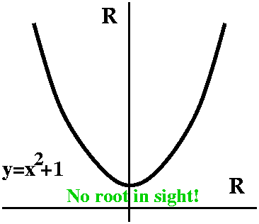 If you want
to have enough numbers so that things intersect correctly you
need the real field. That's the one with all possible decimal
expansions. We have a course (Math 311) mostly devoted to proving everything you'd
want to know about the real numbers using this completeness
assumption. So I don't need to do anything about it. But, sigh, there
is something even simpler that's still wrong. In high school we learn
that polynomials should have roots. So the embarrassment of
x2–2 is dealt with by assuming completeness (the parabola
and the line should intersect!). But a more obvious flaw is
that x2+1 which should clearly (?) have two roots
doesn't have any at all!
If you want
to have enough numbers so that things intersect correctly you
need the real field. That's the one with all possible decimal
expansions. We have a course (Math 311) mostly devoted to proving everything you'd
want to know about the real numbers using this completeness
assumption. So I don't need to do anything about it. But, sigh, there
is something even simpler that's still wrong. In high school we learn
that polynomials should have roots. So the embarrassment of
x2–2 is dealt with by assuming completeness (the parabola
and the line should intersect!). But a more obvious flaw is
that x2+1 which should clearly (?) have two roots
doesn't have any at all!
Correcting the flaw
So the complex numbers, C, correct the flaw. In C, x2+1 (or
z2+1, to use the variable name which is more common) has
two roots, +/–i.
Arithmetic in C
I want to be sure that we can do arithmetic in C. So let me write how
to add and multiply complex numbers.
Suppose z=a+bi and w=c+di. Then:
Addition z+w=(a+c)+(b+d)i. (This is exactly the old
"head-to-tail" definition of vector addition. Good: less need to
enlarge the brain.)
Multiplication Well, if we just try to compute
(a+bi)(c+di) and assume everything will work (distribute, use
i2=–1, etc.), then zw=(ac–bd)+(ad+bc)i. So that's our
definition.
Verification of the field rules in C (eh)
Clearly these rules make C into a field. Well,
maybe not clearly. But I am lazy and verification that C is a field is
tedious. There is one aspect that takes some thinking, so let me
address it, and that's the existence of multiplicative inverses. I
want to show you that if a+bi is not the 0 complex number
(0+0i) then there is another complex number whose product with this
one gives me 1 (1+0i). Here is a way to think about it:
  1       1      (a–bi)        a–bi        a–bi
----- = ----- · -------- = ------------ = ------
 a+bi    a+bi    (a–bi)    (a+bi)(a–bi)    a2+b2
So now I guess that if w=(a/[a2+b2])–(b/[a2+b2])i then the product of z and w will be 1.
Indeed,
a(a/[a2+b2])–b·{–(b/[a2+b2])}=[a2+b2]/[a2+b2]=1
(that's the first part of the product) and
a(–b/[a2+b2])+b·(a/[a2+b2])=[–ab+ba]/[a2+b2]=0
(that's the second part of the product).
Notice, please, that the above computation is successful exactly when
the number a2+b2 is not 0, and this is
exactly when the complex number a+bi is not the 0 complex number,
0+0i.
A sane person might ask what is going on here. Well, my primary answer
would be, "It works, doesn't it?" If that is not satisfactory to you,
then there are a large number of detours I could suggest (study some
algebra -- for example, Math 451-452). But for this course, I will try
to make believability arguments (heuristic discussions). This is
actually how things grew historically.
Vocabulary and pictures
Almost everything that "accidentally" got written above turns out to
have a special name. So if z=a+bi:
- a is called the real part of z, and we write a=Re(z).
- b is called the imaginary part of z, and we write b=Im(z).
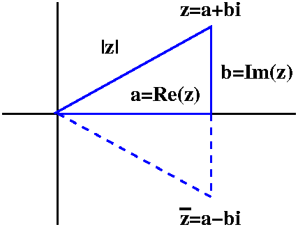 The number sqrt(a2+b2) is written |z|, and
is called (variously) the modulus of z, the norm of
z, the magnitude of z ... I'll probably just use the first word
most of the time. The reason to think about the square root instead of
what's inside is because of the picture to the right.
The number sqrt(a2+b2) is written |z|, and
is called (variously) the modulus of z, the norm of
z, the magnitude of z ... I'll probably just use the first word
most of the time. The reason to think about the square root instead of
what's inside is because of the picture to the right.
Note Square roots are at the core of a great deal of difficulty
in this subject. Right now I will only use sqrt to mean the following:
if V is a non-negative real number then sqrt(V) will mean the
unique non-negative real number which, when multiplied by
itself (its square) gives V. I'll work more diligently to discuss how
we should think about other square roots.
- a–bi is called the complex conjugate of z, and is written z
with a bar over it (in html I will write z) and we sometimes say
z-bar. Geometrically, z is the reflection of z in
the horizontal axis.
Relabeling the pictures
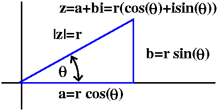 Let's draw things a bit differently and get a polar
representation of z. Then we get the interesting formula
Let's draw things a bit differently and get a polar
representation of z. Then we get the interesting formula
z=r(cos(θ)+i sin(θ)) (somehow I usually write
the i in front of the sine)
Here r is the modulus, and θ is
called the argument of z. And now we are in a great deal of
trouble, because of "the". Actually, there are many arguments which
are valid. We only need the information contained in the values of
sine and cosine of θ, so
arguments are really only defined up to a multiple of 2Π.
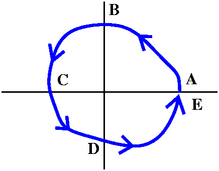 The difficulty
is actually fundamental. Let me show you: let's start with a point on
the positive real axis, A. I guess I could have its argument be
0. Then let us travel around towards B. If I want the argument to
move or vary continuously, then I think that B's
argument should be Π/2. Now let's go to C on the path shown. C is on
the negative real axis, and, to keep things nice, it should have
argument Π. Of course we will move on to D, which should have
argument 3Π/2. Now creep very slowly to E, and E itself is darn close
to A. Well, I bet that E's argument, if we want things to vary
continuously, should be nearly 2Π. But ... but ... if we let E move
to coincide with A, then what should the argument be? Is it 0 or 2Π?
Have we somehow made a mistake? Not at all: this is part of what we
need to explain. If we want to have a continuous argument, then we
will have to agree that argument is defined only up to integer
multiples of 2Π (as math folks might say, "mod 2Π"). This will come
up again below in a more algebraic context. This is a serious
complication which won't go away.
The difficulty
is actually fundamental. Let me show you: let's start with a point on
the positive real axis, A. I guess I could have its argument be
0. Then let us travel around towards B. If I want the argument to
move or vary continuously, then I think that B's
argument should be Π/2. Now let's go to C on the path shown. C is on
the negative real axis, and, to keep things nice, it should have
argument Π. Of course we will move on to D, which should have
argument 3Π/2. Now creep very slowly to E, and E itself is darn close
to A. Well, I bet that E's argument, if we want things to vary
continuously, should be nearly 2Π. But ... but ... if we let E move
to coincide with A, then what should the argument be? Is it 0 or 2Π?
Have we somehow made a mistake? Not at all: this is part of what we
need to explain. If we want to have a continuous argument, then we
will have to agree that argument is defined only up to integer
multiples of 2Π (as math folks might say, "mod 2Π"). This will come
up again below in a more algebraic context. This is a serious
complication which won't go away.
A wonderful computation
Complex number addition is just a rephrasing of the old
(2-dimensional) vector addition. Complex multiplication (with ac–bd
and ad+bc) seems more complicated. Let me show you a neat computation
that might help clarify what is going on.
Suppose z=r(cos(θ)+i sin(θ)) and
w=s(cos(λ)+i sin(λ)). Let's compute zw. We can do
this in any order (associativity) so that
zw=rs(cos(θ)+i sin(θ)) (cos(λ)+i sin(λ))=rs(cos(θ)cos(λ)–sin(θ)sin(λ)+i cos(θ)sin(λ)+sin(θ)cos(λ)).
We accidentally recognize certain things. (In fact, there aren't any
accidents. Later you will see why these computations work as they do.).
zw=rs(cos(θ+λ)+i sin(θ+λ)). Well, cos(thing)+i sin(thing) always has
modulus 1 (because sin2+cos2=1). So:
The consequences
The modulus of the product is the product of the moduli: |zw|=|z||w|.
The argument of the product is the sum of the
arguments.
 These statements
help understand what complex multiplication "does" because the
formulas ac–bd and ad+bc seem complicated. Consider the function
mapping z→iz (that is, multiplication by i). Then the modulus
multiplies, so |iz|=|i| |z|=1 |z|=|z| since i has modulus
equal to 1. Therefore iz must be a complex number on the circle
centered at 0 with radius equal to |z|. What about the
argument? Well, arg(iz)=arg(i)+arg(z)=Π/2+arg(z), so the argument
of iz is a right-angle plus the argument of z. The plus is
important since it tells us that iz is z rotated clockwise by a
right-angle (relative to the origin). So the mapping z→iz is a
rotation by a right angle around the origin.
These statements
help understand what complex multiplication "does" because the
formulas ac–bd and ad+bc seem complicated. Consider the function
mapping z→iz (that is, multiplication by i). Then the modulus
multiplies, so |iz|=|i| |z|=1 |z|=|z| since i has modulus
equal to 1. Therefore iz must be a complex number on the circle
centered at 0 with radius equal to |z|. What about the
argument? Well, arg(iz)=arg(i)+arg(z)=Π/2+arg(z), so the argument
of iz is a right-angle plus the argument of z. The plus is
important since it tells us that iz is z rotated clockwise by a
right-angle (relative to the origin). So the mapping z→iz is a
rotation by a right angle around the origin.
But all this has some difficulties (I'd like to be sort of honest!). I
know that:
i2=–1, and i3=–i, and i4=1.
If we take arg(i) to be Π/2, then arg(i2)=2(Π/2)=Π and
arg(i3)=3(Π/2)=3Π/2 and arg(i4)=4(Π/2)=2Π,
which might contrast interestingly with a naive value of
arg(i4)=arg(1)=0. So 0=2Π? Well, "mod 2Π" or, up to an
integer multiple of 2Π, that's true. We need to keep this in mind. It
will come up again and again.
Maintained by
greenfie@math.rutgers.edu and last modified 1/20/2010.
 One geometric method which helps understand certain conformal mappings
is to visualize what is going on using stereographic
projection. Put the complex plane into space (R3) as
the xy-plane, with third coordinate equal to 0. Draw a sphere with
radius 1 and center the origin, (0,0,0). Let N, the North Pole, be
located at (0,0,1). Then every point a on the sphere which isn't N
corresponds to a unique point b on the complex plane. The
correspondance is by drawing a line from N to a and extending it until
it intersects the plane. The intersection point is called b. Of
course, we could start with b on the complex plane, and connect it
with N, and the line would always hit the sphere in some other point,
a. This "correspondance" is a useful thing to keep in the back of your
mind (?) throughout your study of the subject. Of course you can write
lots and lots of equations describing everything, but right now I just
want the idea, without proofs or whatever. In fact, it turns out that
stereographic project also "preserves angles" between corresponding
curves (this is not immediately obvious at all).
One geometric method which helps understand certain conformal mappings
is to visualize what is going on using stereographic
projection. Put the complex plane into space (R3) as
the xy-plane, with third coordinate equal to 0. Draw a sphere with
radius 1 and center the origin, (0,0,0). Let N, the North Pole, be
located at (0,0,1). Then every point a on the sphere which isn't N
corresponds to a unique point b on the complex plane. The
correspondance is by drawing a line from N to a and extending it until
it intersects the plane. The intersection point is called b. Of
course, we could start with b on the complex plane, and connect it
with N, and the line would always hit the sphere in some other point,
a. This "correspondance" is a useful thing to keep in the back of your
mind (?) throughout your study of the subject. Of course you can write
lots and lots of equations describing everything, but right now I just
want the idea, without proofs or whatever. In fact, it turns out that
stereographic project also "preserves angles" between corresponding
curves (this is not immediately obvious at all).
 The picture I would like you to see is to the right. It has all (or
almost all the information about the rational function, because two
rational functions which have the same zeros and poles can differ only
by a non-zero multiplicative constant!) of the information about the
rational function, but displayed in a rather pleasing and possibly
informative geometric manner. The poles of the
function are "at" the points which have negative integer
weights. The zeros of the function are "at"
the points which have positive integer weights. This assemblage
(?) is called the divisor of the function (I won't use this
word again in this class).
The picture I would like you to see is to the right. It has all (or
almost all the information about the rational function, because two
rational functions which have the same zeros and poles can differ only
by a non-zero multiplicative constant!) of the information about the
rational function, but displayed in a rather pleasing and possibly
informative geometric manner. The poles of the
function are "at" the points which have negative integer
weights. The zeros of the function are "at"
the points which have positive integer weights. This assemblage
(?) is called the divisor of the function (I won't use this
word again in this class).
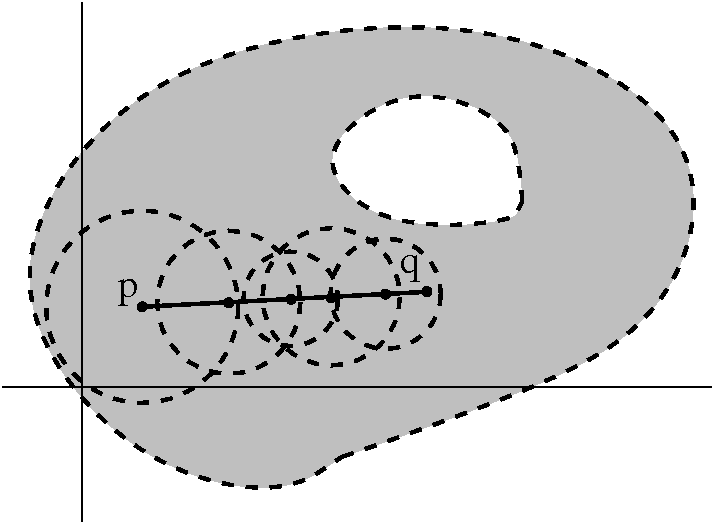 But "identically 0" spreads around the connected open set U. I gave
this argument at least once earlier in the course -- let me
run rapidly through it again. Let's draw a line inside U between p and
q. Since f s 0 near p, the power series expansion for f is 0 inside a
disc centered at p. f and all of its derivatives vanish in that
disc. Now select another point in the disc, moving from p towards
q. Since f and all of its derivatives vanish at that point, I know that the
coefficients of the power series coefficients for f at that point are
all 0. So in a disc centered at that point, f must be identically 0. I
can continue along a chain of discs from p to q, and then f must be 0
in a disc which includes q.
But "identically 0" spreads around the connected open set U. I gave
this argument at least once earlier in the course -- let me
run rapidly through it again. Let's draw a line inside U between p and
q. Since f s 0 near p, the power series expansion for f is 0 inside a
disc centered at p. f and all of its derivatives vanish in that
disc. Now select another point in the disc, moving from p towards
q. Since f and all of its derivatives vanish at that point, I know that the
coefficients of the power series coefficients for f at that point are
all 0. So in a disc centered at that point, f must be identically 0. I
can continue along a chain of discs from p to q, and then f must be 0
in a disc which includes q.
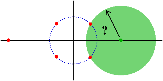 Here is a more subtle problem. Consider the function f(z) defined by
the formula f(z)=ez/{(z+3)(z4+1)}. f(z) is a
function which is analytic with isolated singularities at 3 and at the
fourth roots of –1 (this are, I think,
(±1±i)/sqrt(2). Since in each case we can write an
appropriate factorization in terms of (z–CENTER)–1 times h(z) with h(CENTER)≠0, we know that these singularities
all happen to be "simple poles", or poles of order 1.
Here is a more subtle problem. Consider the function f(z) defined by
the formula f(z)=ez/{(z+3)(z4+1)}. f(z) is a
function which is analytic with isolated singularities at 3 and at the
fourth roots of –1 (this are, I think,
(±1±i)/sqrt(2). Since in each case we can write an
appropriate factorization in terms of (z–CENTER)–1 times h(z) with h(CENTER)≠0, we know that these singularities
all happen to be "simple poles", or poles of order 1.