Math 152H diary, fall 2009
Later material
Much later material
In reverse order: the most recent material is first.
| Wednesday,
October 1 | (Lecture #8) |
|---|
Factoring integers
This is a well-known (yeah,
really) hard problem. The problem is: given a positive
integer, describe it as its (essentially unique up to order) product
of primes. So, for example, 15=3·5, and
221111156722344485686886868684333399999994445 (a 44 digit number) is
this product of primes:
5·173·1339186906073·23060119·8277359364118608174739
which is certainly not obvious, and took a silicon friend of mine
about .7 seconds to "realize".
Polynomial factorization is harder. Sigh. So nothing good is going to
happen theoretically, which is sad because lots of uses for the
partial fraction algorithm are known (for example, in control theory,
a branch of electrical engineering).
Another example or two
The example I did last time ended with 11x+7 divided by
x2–2x–3. The bottom (denominator?) here can be factored
easily as (x–3)(x+1). Let me change the example by changing
the bottom because otherwise the full horror (!) of partial
fractions will not be revealed.
∫(11x+7)/[(x-3)(x+1)(5x+2)]dx?
Well, an integer can have more than two prime factors.
Here is the sort of sum we need to investigate:
     11x+7          A     B      C
---------------- = --- + --- + ------
(x-3)(x+1)(5x+2)   x-3   x+1    5x+2
Let's combine the fractions on the right using the least common
multiple. The right side combines like this:
A(x+1)(5x+2)+B(x-3)(5x+2)+C(x-3)(x+1)
------------------------------------
          (x-3)(x+1)(5x+2)
This is supposed to be equal to the fraction we had above (on the
left-hand side of the equation). Now the bottoms of the fractions are
the same, so the tops must agree. Therefore we know
11x+7=A(x+1)(5x+2)+B(x–3)(5x+2)+C(x–3)(x+1)
Now x=–1 tells me that 11(–1)+7=0+B(–1–3)(–5+2)+0 so we can deduce the
value of B, which is 3. And x=3 tells me that
11(3)+7=A(3+1)(5(3)+2)+0+0 so that A=40/(4·17). Finally, x=–2/5
will let me deduce the value of C. Therefore we get a partial fraction
decomposition of (11x+7)/[(x–3)(x+1)(5x+2)]. Notice that each piece
can be easily antidifferentiated:
∫[A/(x–3)]+[B/(x+1)]+[C/(5x+2)]dx=Aln(x–3)+Bln(x+1)+(C/5)ln(5x+2).
Whew. The only trick is the /5 because of the Chain Rule again.
∫(11x+7)/[(x-3)(x+1)2]dx?
Well, an integer can have repeated prime factors, such
as 175=527.
Now one of the factors has a higher power than 1. Some people say that
–1 is a root of the bottom polynomial which has multiplicity
2. In this
case, the symbolic sum has to be modified. There is one term for each
power going up from 1 to the multiplicity. So here:
  11x+7       A     B      C
---------- = --- + --- + ------
(x-3)(x+1)2  x-3   x+1   (x+1)2
This is step 2, the symbolic sum. Step 3 requires that specific values
be found for A and B and C. What I do here is good for small
examples. So I would combine the fractions on the right-hand side,
using the least common denominator. You need to be careful about this. I have made mistakes lots of times. A B C A(x+1)2+B(x-3)(x+1)+C(x-3)
--- + --- + ------ = ----------------------------
x-3 x-1 (x-1)2 (x-3)(x+1)2
Compare the top of the result here with the top of
(11x+7)/{(x–3)(x+1)2}.
11x+7=A(x+1)2+B(x–3)(x+1)+C(x–3)
I want any method of getting values for A and B and C which
make this equation correct. "Theory" guarantees that there are such
values, and that these values are unique. I can try magic numbers for
x again.
x=–1 gives 11(–1)+7=A·0+B·0+C(–4) so that C=1.
x=3
gives 11(3)+7=A(4)2+B·0+C·0 so that
A=40/16=5/2.
There doesn't seem to be a magic number which will produce B. Here are
some strategies I use for such examples:
One strategy
Take x=0. This isn't magic, but it simplifies things. Then the
equation becomes
11·0+7=A(1)2+B(–3)(1)+C(–3). Since we know A and C we get
7=(5/2)–3B+1(–3) and 7–(5/2)+3=–3B and 15/2=–3B so B=–5/2.
Another strategy
Look at the x2 coefficient on both sides of the equation
11x+7=A(x+1)2+B(x–3)(x+1)+C(x–3).
On the left there are no x2's, so the result is 0. On the
right (be careful!) there are A x2's and also B
x2's (there aren't any from the C term). Therefore 0=A+B
and since A is 5/2, B is –5/2.
These are the same. I needed three tries to get
everything to work out correctly!
The pieces are:
5/2   -5/2     1
--- + ---- + -----
x-3    x+1   (x+1)2
Can we integrate the result? Yes. The first piece gives 5/2ln(x–3) and the second piece gives –5/2ln(x+1). The last part is (x+1)–2 which gives (–1)(x+1)–1.
If (x–root)multiplicity is a factor of the bottom, then in
Step 2 there will be a bunch of parts,
(various constants)/(x–root)integer, with the integer
going from 1 to multiplicity. For example, here is the Step 2 response to the following:
 x4-3x2+5x-7     A       B       C       D       E       F
------------- = ----- + ----- + ----- + ----- + ----- + -----
(x+5)2(x-7)4     x+5    (x+5)2   x-7    (x-7)2  (x-7)3  (x-7)4
And this would lead to a system of 6 linear equations in 6
unknowns. By the way, Step 3, solving the linear equations,
turns out to be computationally quite straightforward. Here I don't
mean doing things by hand, but on a machine. Very big systems (tens of
thousands of linear equations) are solved efficiently on computers
frequently. The reason all of these parts need to be used is because
without them the method just will not work, and you would need
to go into the proof of the algorithm (not part of this course!) in
order to see more clearly what's going on.
There is one more significantly different computational difficulty. I
will discuss it on Wednesday, the next lecture, and complete the
statement of the partial fraction algorithm.
And now another difficulty ...
Because I am only supposed to talk to you about
real calculus, we run into another sort of difficulty which is
not seen at all in factoring integers. In practice, in, say,
engineering applications, people indeed use complex numbers so I don't
need to worry about this sort of thing.
Factoring polynomials is more difficult than we have seen so far. In
addition to linear factors, there are polynomials like
x2+1. This polynomial is never zero, so it can't be
written as a product with any linear x–a (if x2+1
were equal to such a product, when x=a the result would be 0, which
never happens). So let me show an example.
Yet another example
I'll show you the symbolic pieces, and then solve for them.
   11x+7        A      Bx+C
----------- = ----- + ------
(x-3)(x2+1)    x-3     x2+1
So when there is an irreducible quadratic then an unknown
linear term needs to be put on top.
If we combine terms and look at the tops, the result is
11x+7=A(x2+1)+(Bx+C)(x–3).
Again, any method that gets the answer is a good method. So:
x=3 gives 11·3+7=A(32+1)+(Bx+C)0 so 40=10A so A=4.
x=0 gives 7=A(1)+(B·0+C)(–3) so 7=A–3C so since A=4, 7=4–3C and
C=–1.
Consider the x2 coefficients: 0=A+B, so since A=4, B=–1.
Therefore
   11x+7        4     -4x-1
----------- = ----- + ------
(x-3)(x2+1)    x-3     x2+1
Integration
Let's integrate the pieces.
A
small amount of rewriting gives:
   11x+7        4      -4x      -1
----------- = ----- + ------ + -----
(x-3)(x2+1)    x-3     x2+1     x2+1
The first and third terms should not be difficult to recognize and
integrate: 4ln(x–3) and –arctan(x). The middle term can be done with
w=x2+1 so dw=2x dx, with the result
–2ln(w)=–2ln(x2+1). And +C of course. So finally
∫(11x+7)/[(x–3)(x2+1)]dx=4ln(x–3)–2ln(x2+1)–arctan(x)+C.
What is an irreducible quadratic?
An irreducible quadratic is a degree 2 polynomial which has no real
root. So 5x2–9x+17 is an irreducible quadratic but
7x2–88x–20 is not. How do I know this? Well,
the roots of Ax2+Bx+C=0 are given by the famous formula
[(–B+/–sqrt{B2–4AC})/2A]. The roots are
real exactly when the "stuff" under the square root sign in the
formula is not negative. (Negative gives complex roots and I am not
supposed to discuss these with you lest your brains explode.) The
B2–4AC is usually called the discriminant. For
5x2–9x+17 the discriminant is
(–9)2–4(5)(17) sure looks negative and for
7x2–88x–20,
(–88)2–4(–20)7 certainly seems positive.
Geometrically, the graph of a quadratic is a parabola. The roots
represent intersections with the x-axis. It is certainly possible that
the parabola is high up (or high down?) and does not intersect the
x-axis. In that case, the quadratic is irreducible (cannot be
factored).
What we did so far ...
I've tried to explain how partial fractions splits up a rational
function into a sum of pieces which are easier to understand and
analyze. In the context of Math 152, the further work is
antidifferentiation. So we've looked at Top(x)/Bottom(x). First we
divided, if necessary, to get the degree of the Top less than the
degree of the Bottom (the quotient is a polynomial which we already
know about). The result, a proper rational fraction, is what we
will investigate now. The Partial Fractions algorithm depends on
factoring Bottom(x). I've tried to show with examples what to do if
there are linear factors, like (x–3)2
What happens in general
Powers of linear factors need constants on top. Powers of irreducible
quadratics need degree one "unknowns" on top.
The partial fraction algorithm
First there is a theorem which is not part of Math 152. The
theorem states that every rational function has exactly one partial
fraction description. What's below is an attempt to describe how to
get that description.
| Description | Feasibility |
|---|
Step 0 Long division
Take a rational
function, and divide Top by Bottom until there is a Quotient (which
will be a polynomial) and a remainder. Make the remainder the new top,
and then pass that fraction (remainder/Bottom) to the next steps.
| This is certainly easy to do by hand or by machine. |
Step 1 Factoring
Factor the bottom into
powers of linear polynomials and powers of irreducible quadratics.
|
If the factorization is known, everything else is
easy. This is the part that is authentically computationally
difficult. There's a theorem which states that every polynomial
can be written as a product of linear factors and irreducible
quadratic factors. But actually finding these factors, even
approximately, can be a difficult computational task. |
Step 2 Write a symbolic sum
(linear)power: if, say, (x–3)4 is a factor,
write a sum of 4 terms:
k1/(x–3)1+k2/(x–3)1+k3/(x–3)2+k4/(x–3)3. In
general, there are as many terms as the degree of the power of the
linear factor, and each has an unknown symbolic constant on top.
(irred. quad.)power: if, say,
(4x2+5x+11)3 appears, then write
(k1+j1x)/(4x2+5x+11)1+(k2+j2x)/(4x2+5x+11)2+(k3+j3x)/(4x2+5x+11)3. In
general, there are as many terms as the degree of the power of the
irreducible quadratic factor, and each has two unknown symbolic
constants on top, arranged as a linear polynomial.
| This is easy to do, once you get used to it. |
Step 3 Find the values of the
constants
Push together the fractions with the symbolic coefficients. Then if
this is to be equal to the original rational function, the tops must
be equal. Find the values of the symbolic coefficients.
| This actually turns out not to be difficult in practice when
you learn what you are doing. The equations for the symbolic
coefficients are just a collection of linear (first power)
equations in the unknowns. It is easy and practical to solve systems
of linear equations, even very large systems of linear equations
(people deal with systems of thousands of linear equations all the
time!).
|
If you want to include Step 4, integrating the pieces, then you
should already see that integrating the pieces which come from the
linear factors is not difficult. Integrating the pieces which come
from the irreducible quadratic factors can certainly be tedious by
hand, but not actually impossible. A complete-the-square step followed
by a trig substitution (x=(constant)tan(θ) will do it). It won't
be pleasant, but I could imagine doing low degree examples by hand.
The simplest example of an irreducible quadratic is
1+x2. What sorts of pieces do we get if there is a factor
of (1+x2)2 and how can we
antidifferentiate them? Well, we should get
 Ax+B        Cx+D
------  +  --------
(1+x2)      (1+x2)2
We already discussed the Ax+B term. Antidifferentiating it gives
(A/2)ln(1+x2)+Barctan(x). What about the Cx+D term? Well,
split up the fraction. The Cx/(1+x2)2 is sort of
easy. Again, if w=1+x2, and dw=2x dx, etc. then we can
antidifferentiate. The result is –(C/2)(1/(1+x2)). What
about the D term? Well ...
Checking a formula
The following formula is true:
∫(1/(1+x2)2dx=(1/2)(x/1+x2)+(1/2)(arctan x).
Certainly this formula can be checked by
differentiation. We can now see how this formula was created. If
x=tan(θ) then 1+x2=1+(tan(θ))2=(sec(θ))2
and dx=(sec(θ))2dθ. The
integral becomes
∫[(sec(θ))2/(sec(θ))4] dθ.
Some of the secant powers cancel, and since 1/sec is cos, we need to
compute
∫(cos(θ))2dθ. We have done this a large
number of times with double angle formulas, etc. What we got before is
this:
 (1/2)cos(θ) sin(θ)+θ/2+C.
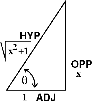
So ... if tan(θ)=x which is x/1 and tan(θ) is also
OPP/ADJ, then I can think of OPP as x and ADJ as 1. See the picture to
the right, please. Then HYP is sqrt(x2+1), and
sin(θ)=x/sqrt(x2+1) and
cos(θ)=1/sqrt(x2+1). Also, θ=arctan(x). So the
whole darn formula in θ-land, (1/2)cos(θ)sin(θ)+θ/2+C, becomes
in x-land this:
(1/2)[1/sqrt(x2+1)][x/sqrt(x2+1)]+arctan(x)/2+C
which is, exactly
(1/2)(x/1+x2)+(1/2)(arctan x), a formula which seemed
so silly that there would be no simple way of finding it. Well, we now
know enough to "discover" such formulas.
An example, not by hand
The following computation took about half a second on my work
computer, which is several years old and not especially fast. I am a
bit surprised it took that long. (Ahhh ... I experimented further:
just loading the appropriate software seems to take most of the time,
not working on the specific example!) The first command defines the
function. The second command asks to convert
the rational function into its partial fraction form. I can't figure
out the order the pieces are printed -- certainly not any order I can
easily identify. All the pieces one might expect according to the
general statement are there, however. Then the third command asks for
the integral (antiderivative) of this. Take a quick look and see which
pieces you can pick out, just for fun. > f:=1/(x*(x-2)^3*(3*x-7)^2*(x^2+4)^2*(x^2+2*x+3));
1
f := ----------------------------------------------
3 2 2 2 2
x (x - 2) (3 x - 7) (x + 4) (x + 2 x + 3)
> convert(f,parfrac);
87 1 -54 - 11 x 59049
-------------- - ------- + ---------------- + ------------------
2 18816 x 2 2 2
30976 (x - 2) 924800 (x + 4) 5967850 (3 x - 7)
-11708 - 1727 x 3774530178 1
+ ------------------ - ---------------------- + -------------
2 104750687125 (3 x - 7) 3
314432000 (x + 4) 1408 (x - 2)
-52145 - 44488 x 8229
+ ------------------------- + --------------
2 681472 (x - 2)
8033987874 (x + 2 x + 3)
> int(%,x);
87 -108 x + 88 14003
- ------------- - 1/18816 ln(x) + ----------------- - --------- arctan(x/2)
30976 (x - 2) 2 628864000
14796800 (x + 4)
19683 1727 2 1258176726
- ----------------- - --------- ln(x + 4) - ------------ ln(3 x - 7)
5967850 (3 x - 7) 628864000 104750687125
1 11122 2
- ------------- - ---------- ln(x + 2 x + 3)
2 4016993937
2816 (x - 2)
1/2
7657 1/2 (2 x + 2) 2 8229
- ----------- 2 arctan(--------------) + ------ ln(x - 2)
16067975748 4 681472
|
Rationalizing substitutions
I showed you how the partial fraction algorithm gets used directly in
integration. But lots of other antiderivatives use partial
fractions because certain substitutions change the integration problem
into the integration of a rational function. Such substitutions are
called rationalizing substitutions. Let's look at a few examples.
∫1/[(2+sqrt(x))(1+sqrt(x))] dx
For this integral, try the substitution u=sqrt(x) because sqrt(x) is
the center of all the trouble or ugliness. Then
du=[1/(2sqrt(x))]dx and so 2sqrt(x)du=dx and 2u du=dx. The
integral ∫1/[(2+sqrt(x))(1+sqrt(x))] dx becomes
∫(2u)/[(2+u)(1+u)] du. This we can easily handle:
(2u)/[(2+u)(1+u)]=A/(2+u)+B/(1+u)=[A(2+u)+B(1+u)]/[(2+u)(1+u)]
So just looking at the tops gives 2u=A(2+u)+B(1+u). u=–1 says A=–2 and
u=–2 says –B=–4 so B=4. Therefore
∫(2u)/[(2+u)(1+u)] du=∫[–2/(2+u)]+[4/(1+u)]du=–2ln(2+u)+4ln(1+u)+C.
We go back to x's and get –2ln(2+sqrt(x))+4ln(1+sqrt(x))+C.
Here's the Maple solution which is what we just got:
> int(1/((2+sqrt(x))*(1+sqrt(x))),x);
                                                   1/2              1/2
                                        -2 ln(1 + x   ) + 4 ln(2 + x   )
Just one more ...
What about ∫[1/(2+sqrt(1+x))] dx? Here I would probably try
u=sqrt(1+x), so that du=[1/2sqrt(1+x)]dx and 2sqrt(1+x) du=dx and
2u du=dx. The integral becomes ∫[(2u)/(2+u)]du.
Now we need Step 0 of the partial fractions algorithm since the degree
of 2u is 1 and the degree of 2+u is 1. So I must divide 2u by 2+u:
       2
    -------
u+2 | 2u
      2u+4
      ----
        -4
So I know that [(2u)/(2+u)]=2+[–4/(2+u)]
(quotient and remainder). I
integrate immediately and get 2u–4ln(2+u)+C and this is
2sqrt(1+x)–4ln(2+sqrt(1+x))+C. This
is correct (I checked it by differentiating). I present the
Maple solution which seems
weird:> int(1/(2+sqrt(1+x)),x);
1/2 1/2 1/2
-2 ln(-3 + x) + 2 (1 + x) + 2 ln(-2 + (1 + x) ) - 2 ln(2 + (1 + x) )
I don't know why the form of the answer is so different and, by the
way, Mathematica supplies the briefer
answer. Professor
Luis Medina is an expert in computational integration
strategies. He has suggested a reason for Maple's answer is a preliminary multiplication
top and bottom by 2-sqrt(1+x). This will lead to the answer given.
QotD
Problem 50 of the partial fractions section of the book asks for
∫(x dx)/[x1/2+x1/3]. The question is: find a
substitution and carry it out so that the result is an antiderivative
of a rational function (you don't need to perform that
antidifferentiation, though!).
I think that the substitution u=x1/6. Well, then
u2=(x1/6)2=x2/6=x1/3. And
u3=(x1/6)3=x3/6=x1/2. Also
u6=x. How about du? One way of getting this is to begin
with u=x1/6 and differentiate: du=(1/6)x–5/6dx,
so that 6x5/6du=dx and 6u5du=dx. Or we could
begin with u6=x and differentiate to get
6u5du=dx. Maybe that way is easier. In any case, we can go
from x-land where we have
∫(x dx)/[x1/2+x1/3] to u-land, where we
get
∫(u66u5du/(u3+u2)=∫6u11du/(u3+u2)
and we can divide by u2 top and bottom to get
∫6u9du/(u+1). Now we would need to divide through
(Step 0) and then go on, but it can be done.
| Monday,
September 29 | (Lecture #7) |
|---|
I mentioned that a rich resource (!)
for the first exam is available.
Just two darn more square root integrals ...
∫01[sqrt(x2–1)/x3]dx
Because I see sqrt(x2–1) and the toolbox contains the
equation (tan(θ))2=(sec(θ))2–1 I will "guess" at the substitution
x=sec(θ), which gives
dx=sec(θ)tan(θ)dθ
and sqrt(x2–1)=tan(θ). With this know, I can rewrite the integral.
∫[sqrt(x2–1)/x3]dx becomes
∫[tan(θ)/sec(θ)3]sec(θ)tan(θ)dθ.
Then cancel everything you can. The result is ∫[cos(θ)]2dθ. We
already considered this integral, The key observation was:
(cos(x))2
can be replaced by (1/2)(1+cos(2x)): the degree is halved, but the
function gets more complicated by doubling the frequency.
so
∫[cos(θ)]2dθ=
∫(1/2)[1+cos(2θ)]dθ=(1/2)[θ+(1/2)sin(2θ)}+C=(1/2)[θ+sin(θ)cos(θ)]+C
using the double angle formula for sine, also in today's toolbox.
 Back to x-land
The translation back turns out to be interesting and more involved
than similar previous transactions. We know that sec(θ)=x and we
want to know what sine and cosine of θ are in terms of x. One way
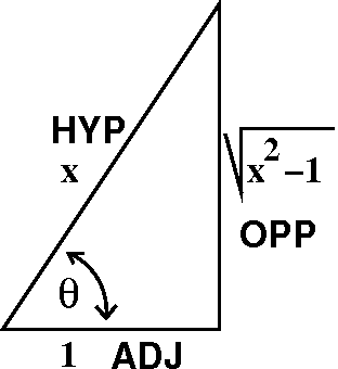
some people use is drawing a right triangle with one acute angle equal
to θ, and with sides selected
so that sec(θ) is x. Since
(with
some effort) we know that secant is ADJACENT/HYPOTENUSE, and we can
think that x is x/1, well the triangle must be like what is
pictured. Then Pythagoras allows us to get the oppositite side, as the
square root of the difference of the squares of the hypotenuse and the
adjacent side. From the triangle we can read off
sin(θ)=sqrt(x2–1)/x
and cos(θ)=1/x. Then
(1/2)[θ+sin(θ)cos(θ)]+C becomes
(1/2)[arcsec(x)+sqrt(x2–1)/x2]+C. As I explained
in class, arcsec is a fairly loathsome function (yes, this is a
value judgment about a morally neutral function).
In fact,
when I asked my silicon friend, the reply was the following:>int(sqrt(x^2-1)/x^3,x);
2 3/2 2 1/2
(x - 1) (x - 1) 1
----------- - ----------- - 1/2 arctan(-----------)
2 2 2 1/2
2 x (x - 1)
That is, Maple does not want to deal
with arcsec at all. Yes, if you really wish, there is a
convert instruction to get the arcsec version. With some
effort, you can look at the triangle and see what arcsec is in
terms of arctan. |
Are we stupid?
We're really not done with the problem. I asked for a definite
integral. Here is what happened to that inquiry on a machine:
>int(sqrt(x^2-1)/x^3,x=0..1);
                                  ∞ I
I wanted to do this specifically to show you the result. The machine
will do (try to do?) what you ask. This is a sort of silly answer, but
the question is, indeed, sort of ridiculous. The integrand is
[sqrt(x2–1)/x3]. On the interval [0,1], the
bottom has x3. I bet that as x→0+, something
weird may happen: the integrand gets very, very large. That explains
the infinity in the result. Later in the course we will see how to
assign certain integrals finite values even when bad things happen to
the integrand, but that procedure won't apply in this case. Where does
the I come from? Well, look at x's inside [0,1]. Those x's make
x2–1 negative and the integrand is requesting the
square root of a negative number. Although we are not supposed to
discuss complex numbers in this course, the machine believes we want a
complex number computation, and it emits (?) an I to indicate this.
So a silly question gets an appropriately silly answer.
A final integral with a square root
The last antiderivative of this type I looked at was something like:
∫sqrt(x2+6x+7)dx.
Here
the novelty is the 4x term. Some algebra which you have likely seen
before can be used to change this to a form we can handle.

Getting rid of the x term
We are "motivated" by the expansion:
(x+A)2=x2+2Ax+A2. We will
complete the square. The picture to the right is supposed to
symbolize this method. Heh, heh, heh ... So:
x2+6x+7=x2+2(3x)+7=x2+2(3x)+32–32+7=(x+3)2–9+7=(x+3)2–2.
Now make the substitution u=x+3 with du=dx. Then
∫sqrt(x2+6x+7)dx
becomes
∫sqrt(u2–2)dt. We can
sort of handle this with a trig substition but there is –2 instead of
–1.
Start with (tan(θ))2=(sec(θ))2–1 and
multiply by 2 to get
2(tan(θ))2=2(sec(θ))2–2. I "guess" that
I would like to try t=sqrt(2)sec(θ). Then
t2=2(sec(θ))2, so t2–2 is
2(tan(θ))2. Also
dt=sqrt(2)sec(θ)tan(θ) dθ. The integral in θ–l and
is ∫sqrt[2(tan(θ))2]sqrt(2)sec(θ)tan(θ) dθ
which is
∫2sec(θ)[tan(θ)]2dθ. As I said in class,
I got bored here. The previous methods can handle this. The details
are complicated and offer lots of opportunity for error. Look below
for a final answer.
Etc.
> int(sqrt(x^2+6*x+7),x);
                      2           1/2
          (2 x + 6) (x  + 6 x + 7)                   2           1/2
          --------------------------- - ln(x + 3 + (x  + 6 x + 7)   )
                       4
I hope you vaguely recognize some of the pieces. For example, the
stuff inside the ln results from ln(sec+tan).
Nice representions of functions
Functions can be studied as the (possibly!) interesting objects that
they are, but it is likely that various kinds of functions will be
used by most students in the class to model physical situations, or to
match data sets. Usually people try to use familiar functions first,
and to use formulas for these functions. In the setting of calculus,
we differentiate and integrate functions. Later, in courses following
calculus which many students will take, other things will be done to
functions (Laplace transforms, Fourier transforms, ...). It is
important to get nice representations of functions,
representations which make it easier to do things with the
functions. This is maybe too darn abstract. Let's look at a particular
example.
Polynomials
Polynomials are probably the first functions anyone thinks about. So I
suggest the following polynomial:
((3+(5+8x3)46)37.
Certainly this is a polynomial. It has degree 5,106. I believe
that I can differentiate it with very little difficulty (two uses of
the Chain Rule). How about antidifferentiation? Well, goodness, we
know how to do that ... but we know how to do that easily when this
polynomial is presented nicely, as a sum of constants multiplied by
non-negative integer powers of x (the standard form of a
polynomial). When I typed a request to integrate something like this
into Maple on either my home or work
computers, all I succeeded in doing was freezing the processors
because, I suspect, the program wanted to e-x-p-a-n-d the presentation
and then antidifferentiate. Much storage and processing was needed to
do that. (Don't try this on a Rutgers computer!)
Rational functions
A rational function f(x) is a quotient, P(x)/Q(x), where the top and
bottom are both polynomials. The aim is not to get a nice
representation of such a function. The best-known representation
is called partial fractions. My aim is to describe the method
of changing "small" examples of rational functions into their partial
fraction representation. I'll also comment, as we go through the
steps, about the computational difficulty of doing this representation
in the "real world". It is true that every rational function has a
unique partial fraction representation, just as every polynomial has a
unique standard representation as a sum of multiples of powers of
x. That there is always a partial fraction representation and there is
exactly one such representation is a theorem. The proof takes a while
and is not part of this course. Describing the process and the type of
result to expect is enough.
The textbook presents the partial fraction representation as an
integration strategy. It is certainly such a strategy, because once
the rational function is written in its partial fraction
representation, antidifferentiation is straightforward. So I will
discuss antidifferentiating the pieces, also. But there are practical
reasons one might want the rational functions decomposed. For example,
the repelling force between two classical charged objects (electrons?)
is rational (it is inverse square where the variable is the
distance between the object). You could imagine that there's a
complicated force law which is rational and has singularities (where
the bottom of the rational function is 0 and the top is not). I might
want to write this as a sum of different forces each with
singularities in only one location. That is always possible and is a
consequence of the partial fraction representation.
An example
I noted that the derivative of ln(x2–2x–3) is not
[(1/(x2–2x–3)] and so therefore the antiderivative of the
latter function is not just the log of the bottom. Then we
wrote [(1/(x2–2x–3)] as a sum of constants multiplying
(x–3)–1 and (x+1)–1 and then got specific values
of the constants. This allows antidifferentiation. As you'll see this
is a typical partial fractions example. But there's one preparatory
step we might have to do which is not included in this example. What
is that?
Suppose I want to look at, say,
[(x3+4x–1)/(x2–2x–3)]. My preparation would
consist of the following:
           x1+2
         ---------------
 x2–2x–3 | x3+0x2+4x–1
           x3–2x2–3x
          --------------
              2x2+7x+1
              2x2–4x–6
             ----------
                 11x+7
So x+2 is the quotient and 11x+7 is the remainder.
We can write the original fraction as:
 x3+4x–1              11x+7
---------- = x+2 +  --------
 x2–2x–3             x2–2x–3
The polynomial is something we know and understand, and it is
correctly "packaged" in a standard way. From now on I'll only consider
proper rational fractions where the degree of the top is less
than the degree of the bottom.
Partial fractions, Step 0
If the input is P(x)/Q(x) and is not proper, then divide the top by
the bottom, and rewrite the result as Quotient+Remainder/Q(x). Here
Quotient will be a polynomial, and Remainder/Q(x) will be a proper
rational fraction. Pass the "Remainder/Q(x)" on to the other steps.
Computational effort of Step 0
This is straightforward, easy to program, and doesn't take much time
or space.
Partial fractions, Step 1, sort of
This step is: given P(x)/Q(x),
find the factors of Q(x). I'll need to say more about this, but look: 6 5 4 3 2
A := 30 x + 179 x - 3859 x - 6591 x + 43369 x + 23500 x - 113652
> factor(A);
(x - 2) (5 x - 11) (x - 9) (2 x + 7) (3 x + 41) (x + 2)
Actually this example is totally silly. I created A by multiplying the
factors which are shown. In reality, factoring is a very
difficult problem.
|
Most of the protocols which guarantee privacy and security in web
transactions rely, ultimately, on the difficulty of factoring, even
the difficulty of finding the prime factors of positive integers. The
most well-known algorithm (RSA, for Rivest-Shamir-Adelman) is based on
the following problem: suppose you know that a positive integer is the
product of two primes. What are the primes? Well, 6 is 2 times 3, so
... except that the numbers are hundreds of decimal digits long, and
there is no known feasible way of finding the integer factors. In the
case of polynomials, the problems are, if anything, even more
difficult, as you will see. The types of factors can vary.
Partial fractions, Step 2, sort of
Write a symbolic sum based on the factorization of the bottom. If we wanted to rewrite (11x+7)/(x2-2x-3), which (11x+7)/[(x-3)(x+1)], the appropriate symbolic sum is
 A     B
--- + ---
x–3   x+1
So there is one term for each factor.
Partial fractions, Step 3, sort of
Find values of the constants in the symbolic sum. In this specific
simple (toy!) example, since
 A     B     A(x+1)+B(x–3)
--- + --- = --------------
x–3   x+1     (x–3)(x+1)
is supposed to be equal to
(11x+7)/(x2-2x-3) because if two fractions are equal with
equal bottoms, then the tops are equal. So we know that
11x+7=A(x+1)+B(x–3)
but then (x=–1) 11(–1)+7=B(–4) so –4=–4B and B=1. And (x=3)
11(3)+7=A(4) so A=40/10=10.
Another way of finding A and B so that 11x+7=A(x+1)+B(x–3) is to
"expand" the right-hand side, getting Ax+A+Bx–3B=(A+B)x+(A–3B). Then
we can look at the coefficients of x and the constant term (the
coefficient of x0) to get
11=A+B
7=A–3B
This is a system of two linear equations in two unknowns and
there are many ways to solve such things. (Hey: A=10 and B=1 are the
solutions of this system!)
|
What's next?
I haven't shown you some further difficulties after the bottom is
factored. I will spend some time with that at the next class meeting,
and then show you also how the partial fractions algorithm comes to be
used at least in many other integration situations.

Algorithm?
I mentioned the word "algorithm". Let
me give some further information about this word in the form of quotes
from
The Art of Computer Programming by D. E. Knuth:
The modern meaning for algorithm is quite similar to that
of recipe, process, method, technique, procedure, routine,
except that the word "algorithm" connotes something just a little
different. Besides merely being a finite set of rules which gives a
sequence of operations for solving a specific type of problem, an
algorithm has five important features:
- Finiteness An algorithm must always terminate
after a finite number of steps.
- Definiteness Each step of an algorithm must be
precisely defined; the actions to be carried out must be rigorously
and unambiguously specified for each case.
- Input An algorithm has zero or more inputs, i.e.,
quantities which are given to it initially before the algorithm
begins. These inputs are taken from specified sets of objects.
- Output An algorithm has one or more outputs, i.e.,
quantities which have a specified relation to the inputs.
- Effectiveness An algorithm is also generally
expected to be effective. This means that all of the operations
to be performed in the algorithm must be sufficiently basic that they
can in principle be done exactly and in a finite length of time.
Knuth continues on the same page to contrast his definition of
algorithm with what could be found in a cookbook:
Let us try to compare the concept of an algorithm with that of a
cookbook recipe: A recipe presumably has the qualities of
finiteness (although it is said that a watched pot never boils), input
(eggs, flour, etc.) and output (TV dinner, etc.) but notoriously lacks
definiteness. There are frequently cases in which the definiteness is
missing, e.g., "Add a dash of salt." A "dash" is defined as "less
than 1/8 teaspoon"; salt is perhaps well enough defined; but
where should the salt be added (on top, side, etc.)?
... a computer
programmer can learn much by studying a good recipe book
|
| Wednesday,
September 23 | (Lecture #7) |
|---|
The first exam for these sections will be in two weeks, either on Wednesday,
October 8 (usual class time and place) or the following day,
Thursday, October 9. I urged students to think about their
schedules and remarked that we would decide tomorrow. Further information,
including extensive review material, will be available very soon.
Now secants and tangents
I want to describe how to find ∫(sec(x))A(tan(x))Bdx if A and B are
non-negative integers. So I will concentrate of how to do this by
hand. You need to know this for exams in Math 152. Again, if I were
describing a method to be implemented by a program, I'd say other
things. Here I will definitely only look at
small A and B because things get very messy rapidly.
What's needed for these functions
Secant &
Tangent
Tools |
d
--- sec(x) = sec(x)tan(x)
dx |
(sec(x))2=(tan(x))2+1 |
|---|
| d
--- tan(x) = (sec(x))2
dx |
(tan(x))2=(sec(x))2–1 |
Imagine this ...
Some maniac has written an infinite list, actually a doubly infinite
list, of functions. The beginning looks like what follows:
                sec(x)             (sec(x))2           (sec(x))3               (sec(x))4

 tan(x)        tan(x)sec(x)     tan(x)(sec(x))2      tan(x)(sec(x))3          tan(x)(sec(x))4

(tan(x))2   (tan(x))2sec(x)    (tan(x))2(sec(x))2    (tan(x))2(sec(x))3       (tan(x))2(sec(x))4

(tan(x))3    (tan(x))3sec(x)   (tan(x))3(sec(x))2    (tan(x))3(sec(x))3       (tan(x))3 (sec(x))4
My goal is to find antiderivatives of all of the functions in this
"list". Since I have only a finite amount of time, maybe what I'll do
is try to convince you that I could find such antiderivatives
by considering a representative number of them. So ...
Early examples
∫(sec(x))2dx=tan(x)+C
∫(tan(x))2=∫(sec(x))2–1 dx
=tan(x)–x+C
I hope that you see even these "low degree" examples have a bit of novelty. Much worse are the first powers!
∫tan(x) dx=∫[sin(x)/cos(x)]dx=∫–(1/u)du=–ln(u)+C=–ln(cos(x))+C=ln(sec(x))+C
where I rewrote tan(x) as sin(x) over cos(x), and then used the
substitution u=cos(x) with du=–sin(x) dx and then got a log and
then pushed the minus sign inside the log by taking the reciprocal of
the log's contents! Horrible.
Much worse, much much
worse, is the following:
What is the derivative of ln(sec(x)+tan(x))? We must use the Chain
Rule. The derivative of the "outside" gives us 1/(sec(x)+tan(x)), and
then we must multiply by the derivative of the inside. But
sec(x)+tan(x) has derivative (look at the secant/tangent tools)
sec(x)tan(x)+(sec(x))2.
Therefore the derivative of ln(sec(x)+tan(x)) is 1/(sec(x)+tan(x))
multiplied by sec(x)tan(x)+(sec(x))2. If you realize that
the top (the second factor) is sec(x) times sec(x)+tan(x), you will
then know that ∫sec(x)dx=ln(sec(x)+tan(x))+C.
After you know this, there are lots of ways of "justifying" this
ludicrous formula. In fact, the formula was not discovered solely by
math people. There is a historical account in the article
An Application of Geography to Mathematics: History of the Integral
of the Secant by Rickey and Tuchinsky appearing in Mathematics
Magazine (volume 53, 1980). Here is a link which will take you
directly to the article if you are on a Rutgers machine.
This "computation" is probably the single most irritating (because of
the lack of motivation) in the whole darn course. The history of this
fact is that it was discovered as a result of the construction of
certain numerical tables used for ocean navigation. This fact is sort
of absurd.
∫(tan(x))4dx
Clearly we can write (tan(x))4 as
(tan(x))2(tan(x))2 and then since
(tan(x))2=(sec(x))2–1, we have
(tan(x))4=(tan(x))2(sec(x))2–(tan(x))2.
So let's compute two integrals:
∫(tan(x))2(sec(x))2dx: if we put
w=tan(x), then dw=(sec(x))2dx, so the integral becomes ∫w2dw=(1/3)w3+C=(1/3)(tan(x))3+C.
We need to subtract ∫(tan(x))2dx, but we just did that. It was
tan(x)–x+C, so the combined result is this:
∫(tan(x))4dx=(1/3)(tan(x))3–tan(x)+x+C.
Neat.
∫(sec(x))3dx
This is also tricky. The first thing is to write it in a rather
strange way:
∫(sec(x))3dx=∫sec(x)·(sec(x))2dx
While you may not think that this helps, it does. Sigh. In fact, "one"
could recognize that
(sec(x))2 is the derivative of tan(x). We can use
integration by parts on this creature. So:
int;(sec(x))3dx=∫sec(x)·(sec(x))2dx=sec(x)tan(x)–∫tan(x)sec(x)tan(x)dx
                   ∫u dv        =    uv    –   ∫v du
where
      u=sec(x)        du=sec(x)tan(x)dx
     dv=(sec(x))2dx    v=tan(x)
How about ∫tan(x)sec(x)tan(x)dx=∫(tan(x))2sec(x)dx?
But (tan(x))2=(sec(x))2–1, so this is
∫((sec(x))2–1)sec(x)dx=
∫(sec(x))3–sec(x)dx=∫(sec(x))3dx–∫sec(x)dx.
Here's the further trick, I think. Suppose we label the integral we want,
∫(sec(x))3dx, by the symbol ♥. Then what we have is
(tricky, tricky):
♥=sec(x)tan(x)–(♥–∫sec(x)dx)==sec(x)tan(x)–♥+∫sec(x)dx.
Just as we did last time, we can "solve" for ♥. This is the
result:
∫(sec(x))3dx=(1/2)(sec(x)tan(x)+ln(sec(x)+tan(x))).
As I mentioned in class, the tricks just shown are enough to allow us
to find antiderivatives of any function on the list we started
with. And with sufficient energy and cleverness, I think a computer
program could be written which would actually find the
antiderivatives. The key would be using certain reduction formulas
(one example is a homework problem). Each step would not be difficult
to do. For example, work similar to what we did before for the integral of (sec(x))3 can be used
to create a reduction formula for (sec(x))n: split into
(sec(x))n-2·(sec(x))2, then integrate by
parts, then use (tan(x))2=(sec(x))2–1 to
get an integral of (sec(x))n and an integral of
(sec(x))n-2 (there are also some numerical
coefficients). Then solve for the desired integral of
(sec(x))n. The result will be some mess (sorry: "some
expression") involving an integral of (sec(x))n-2. Such
formulas are what symbolic computation programs use.
Here is an example from Maple.
< int(sec(x)^9*tan(x)^4,x);
           5                5
     sin(x)           sin(x)           sin(x)          sin(x)
           sin(x)           sin(x)
1/12 -------- + 7/120 -------- + 7/192 ------- + 7/384 ------- +
           7/1536 ------- - 7/3072 -------
           12               10               8               6
           4                2
     cos(x)           cos(x)           cos(x)          cos(x)
           cos(x)           cos(x)

                    3
     - 7/3072 sin(x)  - 7/1024 sin(x) + 7/1024 ln(sec(x) + tan(x))
This computation took about .02 seconds. You must know how to do such
things by hand until after the final exam for Math 152. Then ....
|
Today's tools
We will use the tools we have, with one more equation
whose usefulness will be demonstrated shortly. I will exchange the
previous variable, x, for a new variable, θ, which your text prefers here.
|
Derivative formulas |
Functional equations |
|---|
d
--- sin(θ) = cos(θ)
dθ
d
--- cos(θ) = –sin(θ)
dθ
d
--- sec(θ) = sec(θ)tan(θ)
dθ
d
--- tan(θ) = (sec(θ))2
dθ
|
1=(cos(θ))2+(sin(θ))2
cos(2θ)=(cos(θ))2–(sin(θ))2
sin(2θ)=2sin(θ)cos(θ)
(sec(θ))2=(tan(θ))2+1
(tan(θ))2=(sec(θ))2–1 |
We will use these tools and the ideas we've already seen to
investigate antiderivatives of functions which arise naturally in
physical and geometric problems. The functions involve squares and
square roots.
A circular area
What is the value of
∫01sqrt(1–x2)dx? I truly
expected people to recognize this as a quarter of the unit circle, and
therefore report the value as Π/4. But if we change the upper limit,
then maybe things aren't as simple. So what is ∫01/2sqrt(1–x2)dx?
If I
want to use FTC to compute this, I should find an antiderivative for
sqrt(1–x2). I tried to motivate the following
substitution: x=sin(θ) because
that substitution will make both dx and sqrt(1–x2) come out
"nice". Then dx=cos(θ)dθ and
sqrt(1–x2)=sqrt(1–sin(θ)2)=sqrt(cos(θ)2)=cos(θ). Therefore:
∫sqrt(1–x2)dx=∫[cos(θ)]2dθ.
We use the double angle formula from the toolbox:
∫[cos(θ)]2dθ=∫1/2)[1+cos(2θ)]dθ=(1/2)[θ+(1/2)sin(2θ)]+C
The extra 1/2 comes from the Chain Rule worked backwards on the
"inside" part of cos(2θ). Now I'd like to return to x-land by
writing everything in terms of x instead of θ. Since
sin(θ)=x, we know that arcsin(x)=θ. That allows us to
translate the first part of the answer back to x's. But what about
sin(2θ)? Here is where I need the new formula in the toolbox:
sin(2θ)=2sin(θ)cos(θ). Each of these I already know in
terms of x's because x=sin(θ) and cos(θ) is above (look!): it
is sqrt(1–x2). And we have a formula:
∫sqrt(1–x2)dx=(1/2)[arcsin(x)+x sqrt(1–x2)]+C.
There is cancellation of one of the (1/2)'s with the 2 coming from
sine's double angle formula.
We are not yet done, since we asked for a definite integral.
∫01/2sqrt(1–x2)dx=(1/2){arcsin(x)+x sqrt(1–x2)}|01/2.
Now arcsin(0)=0 and the other term is also 0 at 0, so the lower limit
gives a contribution of 0. The upper limit has
(1/2){arcsin(1/2)+(1/2)sqrt(1–(1/2)2)}. With some thought
we might recall that arcsin(1/2) is Π/6, and also "compute" that
sqrt(1–(1/2)2)=sqrt(3)/2. Therefore the definite integral
is
(1/2)(Π/6)+(1/2)(1/2)(sqrt(3)/2).
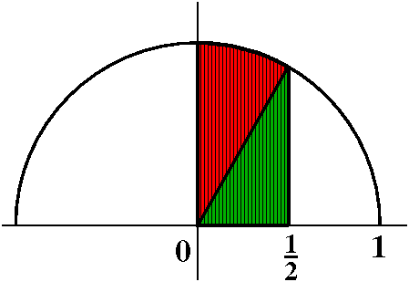 Geometric solution
Actually you can "see" these numbers in the picture.
The triangle has a base whose length is 1/2. Since
the formula for the upper semicircle is y=sqrt(1–x2), the
height of the triangle is sqrt(3)/2. The area of the triangle must
then be (1/2)(1/2)(sqrt(3)/2).
The base acute angle of the triangle is Π/3, so the
circular sector has inside angle Π/6. The area of a circular sector
is (1/2)(angle {in radians!)radius2. Since the radius here
is 1, the area of the circular sector is (1/2)(Π/6).
Maple's version
First the indefinite integral, and then the definite integral.
> int(sqrt(1–x^2),x);
                                 2 1/2
                         x (1 – x )
                         ------------- + 1/2 arcsin(x)
                               2
> int(sqrt(1–x^2),x=0..1/2);
                                   1/2
                                  3       Pi
                                  ---- + ----
                                   8      12
|
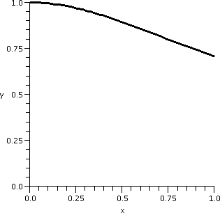
∫011/sqrt(1+x2)dx
I want to compute ∫011/sqrt(1+x2)dx. The value
of
this integral is the area under y=sqrt(1+x2)dx between 0
and 1. A picture of this area is shown to the right. The curve has
height 1 at x=0, and then decreases to height sqrt(1/2) at x=1. Since
sqrt(1/2) is about .7, I know that the definite integral, always
between (Max. value)·(Interval length) and
(Min. value)·(Interval length), is between 1 and
.7.
It is always nice to know some estimate of things to be
computed. That gives us at least a rough way of checking on the
methods and the result. For example, the value of the integral can't
be –17 and it can't be 438. One is negative, and the other is positive
but too large.
How to do it
Look in the toolbox and see
(sec(θ))2=(tan(θ))2+1. If I look at
sqrt(x2+1) then I think of trying x=tan(θ), so
dx=[sec(θ)]2 and
sec(θ)=srqt(x2+1).
Then
∫1/sqrt(1+x2)dx becomes
∫[1/sec(θ)][sec(θ)]2dθ which is
∫sec(θ) dθ. We officially know this integral
because of the ludicrous computation done
earlier.
Its value is ln(sec(θ)+tan(θ))+C. We can
get back to
x-land using what we already know, so the antiderivative we need is
ln(sqrt(x^2+1)+x)+C.
The definite integral computation then becomes:
ln(sqrt(x^2+1)+x)]01=ln(sqrt(2)+1)+ln(1+0)=ln(sqrt(2)+1)
since ln(1)=0. And ln(sqrt(2)+1) is about .88137, certainly between .7
and 1.
Maple's version
You may ask for an antiderivative. Look at the result, which is
slightly surprising:
> int(1/sqrt(x^2+1),x);
                                  arcsinh(x)
What is this? The function called
"arcsinh" is an inverse function to one of the hyperbolic
functions. The hyperbolic functions are discussed in several sections of
the text. They are frequently just as interesting and relevant to
describing and solving problems as the more commonly used trig
functions. The theory is totally parallel. I hope I will have time
later in the course to just show you a bit about them. The trig functions are
connected to the circle, x2+y2=1. The hyperbolic
functions are connected to –x2+y2=1 or
y2=1+x2. There is a Maple instruction which "translates" the
inverse hyperbolic function into things we are supposed to
understand. Here it is:> convert(arcsinh(x),ln);
2 1/2
ln(x + (x + 1) )
The definite integral is recogizable, except for a use of
–ln(A)=ln(1/A) where A=sqrt(2)–1. (You can check that 1/[sqrt(2)–1] is
the same as sqrt(2)+1!) The next instruction finds an approximate
numerical value of the previous answer.>int(1/sqrt(x^2+1),x=0..1);
1/2
–ln(2 – 1)
> evalf(%);
0.8813735879
Another integral
This would have been the QotD but I ran out of time!
Consider ∫[x3/sqrt(1–x2]dx. Again,
if x=sin(θ) this gets converted into a "power of trig functions"
integral. Actually there was little that was new about this integral,
but I thought it would be cute to assign finishing the integral as the
QotD. Here is how to do it.
If x=sin(θ) then dx=cos(θ)dθ and
sqrt(1–x2)=sqrt(1–θ2)=cos(θ) and x3=sin(θ)3 so that the integral
becomes ∫sin(θ)3dθ. In turn we
can "split off" one of the sines, and the result is ∫sin(θ)2·sin(θ)dθ. This makes us think
of the substitution w=cos(θ)
with dw=–sin(θ)d(θ). So the integral changes into
∫(1–w2)–dw
because again sine squared is one minus cosine squared. Now we
{integrate|antidifferentiate} and the result is –w+w3+C (I
pushed through the minus sign) and now back in θ-land we get
–cos(θ)+[cos(θ)3/3]+C and, finally,
back in x-land (we are not done officially until we are back in
x-land!) we get
–sqrt(1–x2)+[{sqrt(1–x2)}3/3]+C.
Just to complete your joy here is what Maple says, and I don't see the process from
the answer: > int(x^3/sqrt(1–x^2),x);
2
(–1 + x) (x + 1) (2 + x )
-------------------------
2 1/2
3 (1 – x )
|
| Monday,
September 21 | (Lecture #6) |
|---|
I wanted to demonstrate some further examples of Integration by Parts.
I asked for courageous volunteers (defined here as "People who didn't
run fast enough") to do the following problems. I thank all of them.
∫ln(x)dx
This problem was done by the volunteers were Mr. Dolinski and Mr. Rusnak. They kindly computed this
(relatively straightforward) antiderivative. If
∫udv=uv–∫vdu, then u=ln(x) implies dv=dx so
du=(1/x)dx and v=x. Then:
∫ln(x)dx=x[ln(x)]–∫x(1/x)dx=x[ln(x)]–∫1dx=x[ln(x)]–x+C.
∫sin(x)sin(3x)dx
Here the vital (!) formulas were obtained by Ms. Bolton and Ms. Little. We want to apply
∫udv=uv–∫vdu to ∫sin(x)sin(3x)dx. This
antiderivative is certainly not as simple as the previous one.
I think the volunteers took parts which were different from the
ones I will use. Here I will try u=sin(x) and dv=sin(3x)dx. Then
du=cos(x)dx and v=–(1/3)cos(3x). Just the computation of v needs
some care, because there is a sign to worry about and then the factor
(1/3) is needed to "fix up" what happens when the Chain Rule
differentiates cos(3x). So ∫udv=uv–∫vdu becomes:
∫sin(x)sin(3x)dx=–(1/3)sin(x)cos(3x)+∫(1/3)cos(3x)cos(x)dx
The plus sign is really two minus signs packaged together. Now things
look bad, because it seems like we have "exchanged" the original
integral for something just as bad. Well, in this case we can try
again. Use integration by parts on ∫cos(3x)cos(x)dx. (I'll pull out the multiplicative factor 1/3
but remember it later!). Take u=cos(x) and dv=cos(3x)dx. The resulting
du is –sin(x)dx and the resulting v is (1/3)sin(3x). The signs and the
multipliers are quite important. The integration by parts formula
becomes:
∫cos(3x)cos(x)dx=(1/3)cos(x)sin(3x)+(1/3)∫sin(x)sin(3x)dx.
We get the original integral back. This plus sign is also two minus
signs. All of the constants are important. Suppose we plug this into
our first Integration by Parts:
∫sin(x)sin(3x)dx=–(1/3)sin(x)cos(3x)+(1/3)((1/3)cos(x)sin(3x)+(1/3)∫sin(x)sin(3x)dx)
Let's call ♠ the antiderivative we want. Then the equation above is:
♠=–(1/3)sin(x)cos(3x)+(1/3)((1/3)cos(x)sin(3x)+(1/3)♠)
so we can solve for ♠.
♠=–(1/3)sin(x)cos(3x)+(1/3)((1/3)cos(x)sin(3x)+(1/3) ♠) is
♠=–(1/3)sin(x)cos(3x)+(1/9)cos(x)sin(3x)+(1/9)♠ so
(1–{1/9})♠=–(1/3)sin(x)cos(3x)+(1/9)cos(x)sin(3x) and since 1–{1/9} is 8/9, we can divide by 8/9 to get
♠=(9/8)(
–(1/3)sin(x)cos(3x)+(1/9)cos(x)sin(3x))
It is not at all clear to me that
∫sin(x)sin(3x)dx=(9/8)( –(1/3)sin(x)cos(3x)+(1/9)cos(x)sin(3x))+C
Comments I just did this antiderivative with
Maple and the result was wonderfully weirdly
different. But more about this later!
The parts chosen in class were different, but the result was the same.
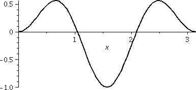 A definite integral
Please notice that sin(x) and sin(3x) are both 0 when x=0 and x=Π
(sines are always 0 at integer multiples of Π). This means (and
this is almost clear, if you assume the antiderivative result above is
correct!) ∫0Πsin(x)sin(3x)dx=0. A
picture of sin(x)sin(3x) on the interval [0,Π] is shown to the
right. Several people helped me with this in class. I thank them
here. Notice that, even with the picture, it is not totally
clear to me that the positive areas (above the x-axis) exactly
balance out the negative area below the axis. They do, though. It
turns out that integrals of this type come up very often when
looking at vibrations of things, and that this integral is 0 (and
other similar integrals, also) is quite useful.
Integer powers of trig functions
The goal today is to show you some algebraic tricks which can be used to compute (in principal!) the
antiderivative of any integer powers of trig functions. I sincerely
hope that you won't have to use these tricks too often once you're out
of Math 152, and that you will have "machinery" available to compute
these integrals. But, as you will see, even with machinery, you will
need to cope with the results, and sometimes they can be irritating to
understand and use.
What's needed
Sine &
Cosine
Tools |
d
--- sin(x) = cos(x)
dx |
1=(cos(x))2+(sin(x))2 |
|---|
| d
--- cos(x) = –sin(x)
dx | cos(2x)=(cos(x))2–(sin(x))2 |
∫sin(x)3cos(x)3dx
This is (relatively) easy, as you will see. What we can do is "borrow"
a cosine, say. What do I mean? Well:
∫(sin(x)3cos(x)3dx=∫sin(x)3cos(x)2[cos(x)]dx
Maybe this suggests the substitution w=sin(x). Then dw=cos(x)dx and we
can write sin(x)3 as w3. What about the last
chunk of the integrand (the function we're integrating)? Well, that's cos(x)2, and since cos(x)2=1–sin(x)2, we see that cos(x)2=1–w2. Now:
∫sin(x)3cos(x)2[cos(x)]dx=∫w3[1–w2]dw=∫w3–w5dw=(1/4)w4–(1/6)w6+C
If we return from w-land to x-land, the answer turns out to be
(1/4)sin(x)4–(1/6)sin(x)6+C.
And another way
An inquisitive person might notice the following: we could have
borrowed a sine. Here:
∫(sin(x)3cos(x)3dx=∫sin(x)2cos(x)3[sin(x)]dx
and take w=cos(x), so dw=–sin(x)dx and –dw=sin(x)dx. Now it is sin(x)2 which we should think of as 1–cos(x)2=1–w2 and replace cos(x)3 by w3, so that:
∫sin(x)2cos(x)3[sin(x)]dx=–∫[1–w2]w3dw=∫w5–w3dw=(1/6)w6–(1/4)w4+C
Things may get a bit tricky. I pulled out a minus first, and then
reinserted it when I multiplied the powers of w inside the
integral. Then I antidifferentiated. So the answer is (substituting
back cos(x) for w here)
(1/6)cos(x)6–(1/4)cos(x)4+C
What's going on?
Let's see: we seem to have two
answers for ∫sin(x)3cos(x)3dx. They are
(1/4)sin(x)4–(1/6)sin(x)6+C
and
(1/6)cos(x)6–(1/4)cos(x)4+C.
If you love (?) trig functions, you know that there are many more trig
identities besides the basic ones listed above in the Sine & Cosine Tools. Maybe the functions
(1/4)sin(x)4–(1/6)sin(x)6 and
(1/6)cos(x)6–(1/4)cos(x)4 are
actually the same.
Plug in x=0 as suggested by Ms. Arya. Then
(1/4)sin(x)4–(1/6)sin(x)6 becomes 0 (hey:
sin(0)=0) and (1/6)cos(x)6–(1/4)cos(x)4
becomes 1/6–1/4 because cos(0)=1. And 1/6–1/4 is
not 0. What is going on here? Let me in fact make things more
difficult before explaining more.
And Maple's answer ...
Let's see what we get:
> int(sin(x)^3*cos(x)^3,x);
                                 2       4              4
                      –1/6 sin(x)  cos(x)  – 1/12 cos(x)
This seems to be different from both of the previous answers. Actually
things aren't that bad because if you substitute 1–cos(x)2
for the sin(x)2 the answer becomes the cosine answer, but
Maple chooses to write the answer this
way. I still haven't answered: What is going on here?
∫x(x+1)dx
So let me try to integrate something really really simple and get two
"different" answers. It will be an artificial example. How can we find
an antiderivative of x(x+1)? Well, a sane human being would multiply
and get x2+x and then integrate to get
(1/3)x3+(1/2)x2 (+C). A crazy person (or a
computer trying to follow a badly implemented algorithm) could do
the following: integrate by parts. So:
∫x (x+1)dx=(1/2)x(x+1)2–∫(1/2)(x+1)2dx=(1/2)x(x+1)2–(1/6)(x+1)3.
    udv   =   uv – vdu
 u=x        du=dx
dv=(x+1)dx  v=(1/2)(x+1)2
I chose to integrate by parts with fairly silly parts. It is all
legal: silly but legal. Certainly one antiderivative of (x+1)
is (1/2)(x+1)2 and then a valid antiderivative of
that is (1/6)(x+1)3 (check them both by
differentiating!).
Therefore (1/3)x3+(1/2)x2 and
(1/2)x(x+1)2–(1/6)(x+1)3 must both be
antiderivatives of x(x+1). Please notice that the first answer has
value 0 when x=0 and the second answer has value –1/6 when x=0, so
these are distinct functions! Is there a problem? Actually, no. Here
theory (if you remember MVT) says you can have infinitely many (not
just 2!) distinct antiderivatives of one function, provided they
differ by a constant. And, indeed, algebra shows exactly this:
(1/2)x(x+1)2–(1/6)(x+1)3=
(1/2)x(x2+2x+1)–(1/6)(x3+3x2+3x+1)=
(1/2)x3+x2+(1/2)x–(1/6)x3–(1/2)x2–(1/2)x–(1/6)=
(1/3)x3–(1/2)x2–(1/6)
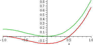
Huh? (and a picture)
The two graphs are parallel to each other. To the right is a graph of
both (1/3)x3+(1/2)x2 and
(1/2)x(x+1)2–(1/6)(x+1)3.
Of course this example is maybe quite silly, but if you use computer
algebra systems, you've always got to remember that "different"
answers can both be valid! A computer program can't always be relied
on to give sensible (?) answers. |
 |
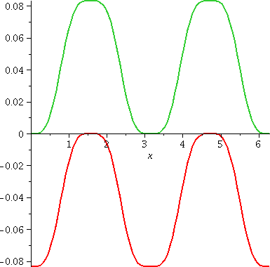
Back to explaining ∫sin(x)3cos(x)3dx
To the right is a graph of the two different antiderivatives of
sin(x)3cos(x)3 on the interval [0,2Π]. I think
that (1/4)sin(x)4–(1/6)sin(x)6
is in green and (1/6)cos(x)6–(1/4)cos(x)4 is in
red and if you believe in pictures, you can see that these
curves are parallel also: they differ by a constant. So you and a
friend who algebraically work on antiderivatives of functions may well
come up with superficially different answers, and both of them
may be correct!
This is weird and wonderful.
| 
|
What about definite integrals?
What happens to the values of definite integrals since we
usually find antiderivatives in order to use FTC (Fundamental Theorem
of Calculus). So let me try to explain, please.
When we apply FTC to evaluate a definite integral,
the setup is something like this:
We have a function F with F´=f and want to know the integral of f
from a to b. We compute F(b)-F(a). Indeed, EXACTLY as you suspect, an
additive constant cancels out. So if we used a function G(x) defined
by F(x)+37, then G´=f also and
G(b)-G(a)={F(b)+37}-{F(a)+37}=F(b)-F(a). So the additive constants
don't matter in this case.
O.k., so how do they affect answers? Well, let's go to a simple
physical example. Suppose f(t) is the velocity of a particle moving on
the horizontal axis: positive means the particle is moving right and
negative means the particle is moving left. That is probably not a
difficult setup. What does a function F(t) with F´(t)=f(t)
represent? Well, this now gets a bit delicate. I know (from the
reasoning above) that F(b)-F(a) doesn't depend on the particular
additive constant. That represents the displacement (the net
change in position) of the particle during the time interval from t=a
to t=b. But if you don't tell me more, then I can't tell you what F(t)
represents. It may or may NOT represent the position of the particle
at time t. IF you tell me an initial position, so that you specify,
say, F(0)=-42, then I can evaluate the +C and then the data (initial
position as well as velocity) will tell us in this model what the
positions are at later times. And F(t), the specific F(t) mentioned,
will be that position.
We will return to specifying initial positions later (in fact, the
whole idea is rather important in applications).
∫sin(x)3cos(x)2dx
This is easy. "Borrow" a sine, convert everything into cosines using a
formula, etc. Things are easy when there is at least one odd
power. But:
∫sin(x)2cos(x)2dx
Now everything is different. If I borrow, what remains can't be
written very nicely in terms of the candidate substitution. A
different trick is used. It converts squares of sines and cosines to
first powers but it doubles the frequency. Here is what I mean:
Look at the tools. We have
1=(cos(x))2+(sin(x))2
cos(2x)=(cos(x))2–(sin(x))2
Add the equations and divide by 2. The result is (1/2)[1+cos(2x)]=cos(x)2.
Subtract the equations and divide by 2. The result is (1/2)[1–cos(2x)]=sin(x)2.
Let's use these equations in ∫sin(x)2cos(x)2dx. So we get ∫(1/2)[1–cos(2x)](1/2)[1+cos(2x)]dx. We
started out with degree 2+2 and now we have degree 1+1, but the
argument in the cosine is 2x, not x. Next, multiply:
∫(1/2)[1–cos(2x)](1/2)[1+cos(2x)]dx=
(1/4)∫1–cos(2x)2dx
and I pulled out the two 1/2 multiplicative factors to get the
1/4. But now we have cos(2x)2 and what shall we do? A burst
of genius (not really, but there is some inspiration!) turns
(1/2)[1+cos(2x)]=cos(x)2 into
(1/2)[1+cos(4x)]=cos(2x)2. (Halve the exponent and double
the frequency!) So:
(1/4)∫1–cos(2x)2dx=
(1/4)∫1–(1/2)[1+cos(4x)]dx.
I can "do" each of the pieces (although I got the constants confused in class!). The answer is
(1/4)(x–(1/2)[x+(1/4)sin(4x)])+C.
Incidentally, Maple's answer is the same
as this one, except (sigh) it is written differently: 3
–1/4 sin(x) cos(x) + 1/8 sin(x) cos(x) + x/8
I know it is the same since both answers have value 0 when x=0. The
"constant" that separates them is therefore 0.
Reduction formula
Here is probably what Maple uses on powers of sine.
Since
∫(sin(x))ndx=
∫(sin(x))n–1 sin(x)dx we can do this:
∫(sin(x))n–1 sin(x)dx=(sin(x))n–1{–cos(x)}–(n–1)∫(–cos(x))(sin(x))n–2cos(x)dx
        udv          =       uv          –        vdu
     u=(sin(x))n–1         du=(n–1)(sin(x))n–2cos(x)dx
    dv=sin(x)dx            v=–cos(x)
But the integral you get "out" is
(sin(x))n–1{–sin(x)}–(n–1)∫(sin(x))n–2(cos(x))2dx) and since
(cos(x))2 is the same as 1–(sin(x))2, you can
"solve" for the original integral. This does work. I think the result
is:
∫(sin(x))ndx=
(1/n)(sin(x))n–1{–cos(x)}+[(n–1)/n]∫(sin(x))n–2dx
I wouldn't use this strategy by hand for small powers of n, but it is
lovely for a program to "know". You can see this reduction formula
being used:> int(sin(x)^9,x);
8 6 16 4
–1/9 sin(x) cos(x) – 8/63 sin(x) cos(x) – --- sin(x) cos(x)
105
64 2 128
– --- sin(x) cos(x) – --- cos(x)
315 315
|
QotD
What is ∫sin(x)3cos(x)2dx?
Hey, isn't this an antiderivative which was called "easy" earlier? Huh. Nasty, nasty, nasty lecturer.
| Wednesday,
September 16 | (Lecture #5) |
|---|
Numerical stuff ...
Also,
I included in the diary for the last lecture details about computing approximations and
error estimates for one specific definite integral. I didn't have
time to do this in class, and this may be helpful for you when
preparing homework problems or workshop solutions or studying for
exams. I also did not discuss the Midpoint Rule, but details about
that are in the book.
Now we'll begin a major part of the course dealing with the symbolic
(not numerical) computation of antiderivatives. The word
"antiderivative" is long, and so I'll use the shorter word
"integral".
There are two methods more important than any others.
Substitution which is the counterpart of the Chain Rule. In
first semester calculus you saw some simple uses of substitution. We
will show some more sophisticated substitutions later in the course.
Integration by Parts is the integration counterpart of the
Product Rule. We'll discuss it today. This method has some rather
surprising consequences which aren't immediately clear with the first
examples.
There are also some miscellaneous algebraic tricks which help find
many integrals, and we'll see them later.
Meeting integration by parts
The derivative of u(x)v(x) is u´(x)v(x)+u(x)v´(x). So this
has to be also an integration formula. Let's see:
∫(u´(x)v(x)+u(x)v´(x))dx=u(x)v(x)
but even that looks a little bit silly. The left-hand side is
also
∫u´(x)v(x)dx+∫u(x)v´(x)dx. That doesn't seem neat. But here is another
way of writing the same equation:
∫u(x)v´(x)dx=u(x)v(x)–∫u´(x)v(x)dx
where we took one of the integrals and put it "on the other
side". This is the formula for Integration by
Parts. The u and v letters are used by almost everyone. There
is also some standard abbreviation which most people use. It's this:
v´(x) is dv/dx, so v´(x)dx=dv. And du=u´(x)dx. Then the
formula becomes more compact and easier to remember:
∫udv=uv–∫vdu
which is very telegraphic. The remainder of the lecture is a sequence
of examples.
Example #0
∫exdx=ex+C. Well, that's not too
illuminating. Let me try something a bit more complicated.
Example #1
How about ∫xexdx. Notice, please, that integration is NOT
multiplicative. While the integral of x is (1/2)x2 (yeah,
yeah, +C), the integral of x2=x·x, is
not {(1/2)x2}·{(1/2)x2} (the degree is wrong, the constant is wrong, and the idea
is wrong!). So we need a new trick, and this new trick is
Integration by Parts. I tend to think of Integration by Parts whenever
I see a product of functions that somehow seem unrelated to each
other, "like" x and ex. Your intuition will develop as you
do more and more examples.
Here I will take u=x and dv=exdx. I will need du, which is
dx, and v, which is ex. I can do the derivative and the
integral "on the fly" -- this is the first real example. Then
∫udv=uv–∫vdu becomes
∫xexdx=xex–∫exdx=(easy to
finish!)xex–ex+C.
Comments
Before jumping forward to other examples, let me analyze this
"easiest" example first.
Comment A Is the result correct? Well, the method says that
xex–ex+C is an antiderivative of
xex. Should we believe this, or, better, is there a way of
checking the result. Well, certainly: differentiation is almost always
easier than integration (antidifferentiation). So let us d/dx the
result:
d/dx(xex–ex+C)=d/dx(xex)–d/dx(ex)+d/dx(C)=(ex+xex)–ex+0=xex.
This shouldn't be so amazing, after all, since integration by parts
and the product rule are inverses of each other. Integration by parts
just arranges things well.
Comment B This is a relatively easy example. There aren't many
possibilities for the "parts". Certainly there will be more choices in
other cases.
Comment C This is my feeling about Integration by Parts:
I have udv, and then I trade it in for vdu, "paying" a penalty of
uv. The idea is that the uv cost allows you to change the function you
need to integrate. As soon as you select, say, u, you then have dv,
and you can sometimes look forward and "see" vdu. You will be
successful if that is somehow simpler or easier than the starting
integral. Machines are fairly good at this, but, honestly, experienced
human beings are even better!
Example #2
Let's do ∫x2exdx. (I am trying to build a
hierarchy of examples, moving from easy to more difficult.) Here try
(although there are other choices!) u=x2 and
dv=ex. Then we need du=2xdx and v=ex. I
mentioned in class and I want to restate here: even when I am alone,
and don't need to teach, I tend to write out all of the
details, including explicit descriptions of u and dv and du and v and
then the Integration by Parts formula. I have found that if I am lazy
and don't do this, then disaster (errors!) occur far too often, and I
just spend more time, because I need to do the computation again and
again. So ∫udv=uv–∫vdu becomes
∫x2exdx=x2ex–∫2xexdx.
What about
∫2xexdx? We can pull out the multiplicative
constant 2 and just get
2∫xexdx. But we know what that integral is -- we just
computed it! Therefore
∫x2exdx=x2ex–∫2xexdx=x2ex&ndash2(xex–ex+C)
The final result would usually be written
x2ex–2xex+2ex+C
and there are a few more things to declare about this. First, notice
that even in this still relatively simple computation several minus
signs occur. There will be a plethora of minus signs as we use
integration by parts. The word plethora is a great SAT
vocabulary work, and one meaning is "A superabundance; an excess". The
minus signs are very easy to get confused about. A second thing is the
apparent silliness of "–2 multiplying +C" becoming just
"+C". Everyone does that. This just means an additive constant, and
its specific name doesn't matter. I think 3C and –5C etc. will
all get renamed +C during this semester during antidifferentiation
exercises.
Example #3
Let's do ∫x3exdx. As I began to address this
problem, I was aware of some unrest in class. So I abandoned the
problem entirely, and decide instead to do
Example #n
Suppose n is a positive integer.
What can we say about ∫xnexdx? Well, if u=xn and
v=exdx, then du=nxn–1dx and v=ex. And
∫udv=uv–∫vdu becomes
∫xnexdx=xnex–n∫xn–1exdx.
No, I have not told you a formula for the antiderivative, but
what I have done is explore the whole collection of integrals, and I
hope that I have convince you that I could compute any specific
"instantiation" of this collection (so I could find an antiderivative
of x5ex or even x123ex).
This sort of setup is called a reduction formula. In its
simplest manifestation, there are a sequence of integrals, and the
reduction formula shows how to work your way down the
sequence. Properly speaking, you ought to also know how to do the
lowest member of the sequence, which we do: that would be
∫xexdx or ∫exdx, both of which we know how to do.
I mentioned ∫x20exdx in class. Here is what
my silicon pal reports when asked for this antiderivative:
 /                                                                   2
 \2432902008176640000 - 2432902008176640000 x + 1216451004088320000 x

                          3                       4                      5
    - 405483668029440000 x  + 101370917007360000 x  - 20274183401472000 x

                        6                    7                   8
    + 3379030566912000 x  - 482718652416000 x  + 60339831552000 x

                     9                 10                11               12
    - 6704425728000 x  + 670442572800 x   - 60949324800 x   + 5079110400 x

                 13             14            15           16         17
    - 390700800 x   + 27907200 x   - 1860480 x   + 116280 x   - 6840 x

           18       19    20\
    + 380 x   - 20 x   + x  / exp(x)
Certainly I can't check the "fine structure" of this formula by just
looking at it. But, roughly, I see certain alternations of sign, and
also the structure of ex multiplied by a polynomial of
degree 20. I sort of expect this, so I am "happy".
|
Example #7
Let's try ∫arctan(x)dx. If you are new at this game, this
integral is quite puzzling. Hey: this is the Integration by Parts
lecture, so we should compute this integral using integration by
parts. So the integrand, what's inside the integral sign, must be
udv. What? Well, there are not many choices. In fact, I can only see
one choice, and maybe it won't be too good: u=arctan(x). Then dv=dx,
so that v=x. And du=[1/{1+x2}]dx (you must know the
basic facts totally well, or you won't be able to get started!). So
∫udv=uv–∫vdu becomes
∫arctan(x)dx=arctan(x)·x–∫x[1/{1+x2}]dx.
This example is slightly more realistic. We now need to compute
∫[x/{1+x2}]dx so the integral we get in exchange for
the original one is not at all "clear".
What is ∫[x/{1+x2}]dx? Actually, this can be computed with a
fairly straightforward substitution. I will use w for the substitution
variable since u is used almost always in the Integration by Parts
formula. Well, if w=1+x2 (the worst part of the integrand!)
then dw=2x dx. We don't have 2x dx, but we do have
x dx. So (1/2)dw=x dx, so that:
∫[x/{1+x2}]dx=(1/2)∫[1/w]dw=(1/2)ln(w)+C
You must learn to be totally sure about simple antiderivatives,
such as the very last step. Now substitute back to get
(1/2)ln(1+x2)+C. The final result is
∫arctan(x)dx=arctan(x)·x–((1/2)ln(1+x2)+C)
so that the antiderivative of arctan(x) is actually
x·arctan(x)–(1/2)ln(1+x2)+C.
Example #8
I tried a definite integral, just to change pace a bit. What is
∫01x·sqrt(1–x)dx? First I'll get
an antiderivative.
So we need ∫x·sqrt(1–x)dx. I don't think that choosing a
"successful" u and dv pair is totally clear here. If u=sqrt(1–x), then
dv=xdx, so v=(1/2)x2, and (I can do this!) du would be some
stuff like –(1/2)(1–x)–1/2. The vdu we would get looks
worse or more complicated than the original. So I don't like this
choice. What if we try u=x and dv=sqrt(1–x)dx? Well, du=dx. If
dv=sqrt(1–x)dx, then I need to make an auxiliary computation:
sqrt(1–x)=(1–x)1/2, and ∫(1–x)1/2dx=–∫w1/2dw (if 1–x=w, so –dx=dw and dx=–dw). Now
∫w1/2dw=(2/3)w3/2 (yeah, yeah, +C). So
(don't forget the minus sign!) ∫(1–x)1/2dx=–(3/2)(1–x)3/2. Wow.
Therefore v=–(3/2)(1–x)3/2. Then
∫udv=uv–∫vdu becomes
∫x·sqrt(1–x)dx=–x(2/3)(1–x)3/2+∫(2/3)(1–x)3/2dx.
The last integral, ∫(2/3)(1–x)3/2dx, we can do with the substitution
w=1–x. The answer will be –(2/3)(2/5)(1–x)5/2. Now put
things back together. Here is the final result.
∫x·sqrt(1–x)dx=–(2/3)x·(1–x)3/2–(4/15)(1–x)5/2+C.
I wouldn't want to check the answer by differentiating! What a
mess. And I made the minus sign larger, because that error is
embarrassingly easy to make: it is three minus signs concatenated, and
I have fouled up such signs too many times myself.
We wanted a definite integral. The antiderivative is so confusing that
I wanted to be able to check the answer. What should the answer "look
like"? Here is a bunch of pictures. If you think through them, I hope
you will see that the answer should be a positive number, certainly
less than 1. (The bump is not symmetric, since sqrt is steeper than x,
certainly.)

The definite integral
∫01x·sqrt(1–x)dx=–(2/3)x·(1–x)3/2–(4/15)(1–x)5/2|01=0(from x=1)–(–4/15)(from
x=0)=4/15.
There are many opportunities for sign errors in this computation.
Another way
Suppose we want ∫x·sqrt(1–x)dx. Hey: just directly try the substitution
w=1–x. Then dw=–dx, and, since w=1–x, solve for x to get x=1–w. The
integral changes:
∫x·sqrt(1–x)dx=∫(1–w)·sqrt(w)(–dw)=–∫w1/2–w3/2dw=–((2/3)w3/2–(2/5)w5/2)+C=–((2/3)(1–x)3/2–(2/5)(1–x)5/2)+C.
The two antiderivatives we got are here:
–(2/3)x·(1–x)3/2–(4/15)(1–x)5/2 and
–((2/3)(1–x)3/2–(2/5)(1–x)5/2)
I think these are the same functions, but the algebra needed is
irritating. I can do it with calculus, though, in a second. Both of
these are antiderivatives of the same function. They must differ by a
constant (+C). If we plug in x=1, both of them are 0. So the +C is 0,
and they are the same!
By the way, here is what Maple tells me: > int(x*(1–x)^(1/2),x);
3/2
2 (2 + 3 x) (1 - x)
- ----------------------
15
Funny, huh (again, the same function, but written differently again!).
|
Example #9
Look at ∫sin(ln(x))dx. The
integrand here is an absurd function. It is NOT a product, but
a composition (read carefully!). It really does occur in applications
(really real applications).
You'll see it again when you study certain kinds of differential
equations. Since this is the Integration by Parts lecture, we should
compute using Integration by Parts (startling). Again, not many
choices, so take u=sin(ln(x)) and dv=dx, so v=x and
du=cos(ln(x))(1/x)dx (use the Chain Rule correctly) and ∫udv=uv–∫vdu becomes
∫sin(ln(x))dx=sin(ln(x))·x–∫x·cos(ln(x))(1/x)dx=sin(ln(x))·x–∫cos(ln(x))dx
because the x and 1/x cancel. We don't seem to have made any progress,
but in fact, be courageous.
Do Integration by Parts again, this time
for ∫cos(ln(x))dx, with u=cos(ln(x)) and
dv=dx. Then du=–sin(ln(x))(1/x)dx and v=x, so
∫udv=uv–∫vdu becomes (be careful!)
∫cos(ln(x))dx=cos(ln(x))·x–∫x·[–sin(ln(x))(1/x)]dx=cos(ln(x))·x+∫sin(ln(x))dx
Suppose we push the formulas together carefully.
∫sin(ln(x))dx=sin(ln(x))·x–∫cos(ln(x))dx=
sin(ln(x))·x–(cos(ln(x))·x+∫sin(ln(x))dx)
This is so very very very tricky. The original integral appears on
the other side with an opposite sign!
∫sin(ln(x))dx=sin(ln(x))·x–(cos(ln(x))·x+∫sin(ln(x))dx)=sin(ln(x))·x–cos(ln(x))·x–∫sin(ln(x))dx
Therefore we can solve for the original integral by taking the
minus indefinite integral to the other side and dividing by 2. Here is
the result:
∫sin(ln(x))dx=(1/2)[sin(ln(x))·x–cos(ln(x))·x]+C.
Check the result if you like by differentiating. This is a ludicrous
and wonderful example.
QotD
Find ∫arcsin(x)dx. Remember that the derivative of the arcsine
function is 1/sqrt(1–x2).
| Monday,
September 14 | (Lecture #4) |
|---|
Definite integrals
These topics are covered in the first chapters of the text:
Chapter 6: Area, Volume, Density, Average Value, Work, Energy
Chapter 8: Fluid Pressure, Arc Length, Surface Area, Center of Mass
We have discussed a few of them and we will discuss a few more (but
not all). The text shows that computing these quantities all involve
evaluating definite integrals. There are many topics covered later in
the text (and in many other courses and situations) which also result
in definite integrals. The next few weeks of the course are an
introduction to some of the methods that people expect you to know
when you are confronted (?) with an integral. There's lots more, but
this is the basic stuff.
What to do? Some alternatives ...
So someone comes up to you on the street and says, "What's ∫ab f(x)dx?" Here
if you're lucky the integrand, f(x), is some easily recognized
function. There are a bunch of algebraic tricks which may be helpful,
and we will begin to study them next time. But if this is the real
world, maybe all you need to know is some numerical approximation
to the value of the integral.
Numerical computation
Scientific and technical computation is present everywhere. The
algebraic tricks we'll see don't always work and sometimes all you can
do is get an approximate value.
|
Computer processors and memories have been improving in speed and size
respectively very quickly over the last 40 years, but studies made of
standard engineering problems requiring lots of computation show that
the speedups which have come about resulted equally from faster
processors and from advances in the computational algorithms.
|
You should know something about the algorithms. Yeah, much of the time
you will (as I do!) just essentially "push a button" to get an
approximate value. But some of the time, perhaps when you least want
to worry about it, your method of choice may not work too well. So you
should have some background knowledge. That's what we will do
today. The two most important considerations are certainly how easy the method is to use, and how accurate it is.
The very beginning ...
I'll show you three methods of approximating definite integrals. The
first is one you sort of know already, but I want to discuss it more
quantitatively. The second and third methods are quite practical, and
if you wanted to, you could actually compute fairly well with
them. Programming them is not too hard. I will admit, though, that
what I show you here is actually not what is used in, say, most
hand-held devices (such as graphing calculators). Somewhat more
elaborate (sophisticated?) methods are used there.
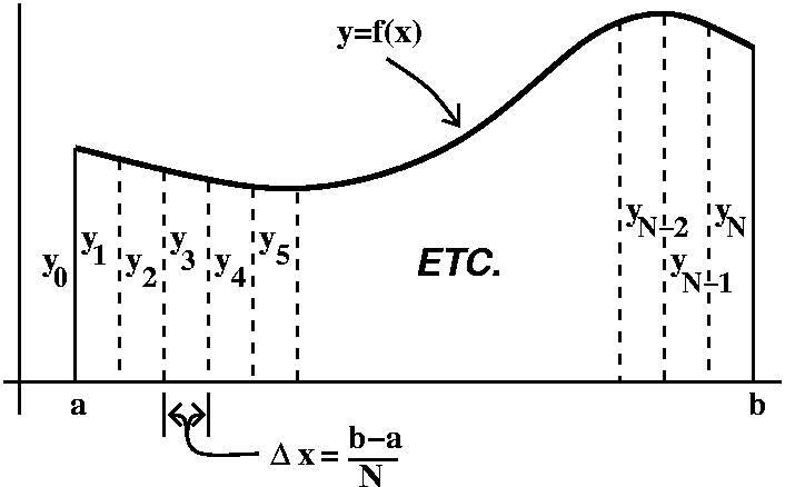
I'm going to try to use the notation in the text. So we'll investigate
the definite integral of f over the interval [a,b]. For all three
methods, we will chop up the interval into equal subintervals, say N
subintervals (you're supposed to think that N will be large). Since
the length of the whole interval is b–a, the length of each
subinterval will be (b–a)/N. We will call this
Δx.
There are N subintervals. The function, f(x), will have N+1 values at
all of the endpoints of all of the subintervals. (There's one more f
value then there are subintervals.) The function values will be
labeled y0, y1, y2, .... up to
yN. The y-value before the last one will be
yN–1. And, if you desperately wanted to know it,
y2, for example, is f(a+2Δx)=f(a+2(b–a)/N).
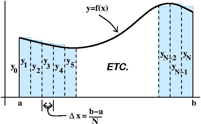 Level 0: Riemann sums, the definition
Just approximate each piece by a rectangle. This is just the Riemann
sum, which appeared in the definition of definite integrals. The side
that's used doesn't matter very much, but to be specific here I'll
choose the left-hand endpoint and evaluate f there, and then multiply
it by the length of the subinterval.
|
Error estimate
 What turns out to be important in this business is,
first, how much work is the computation, and second, what sort of
error estimate is valid. Let me copy what I did in class. I looked at
an interval from 0 to small, so you should think of this as a very
narrow interval (yeah, but the picture ...).
The true value of the integral is ∫0smallf(x)dx. The rectangle
approximating is has height f(0), the value on the left-hand endpoint,
multiplied by the width of the subinterval, small. This is
f(0)·small. But notice that this is also an integral: ∫0smallf(0)dx
(there is no x in this integrand!). So here is the error:
∫0smallf(x)dx–∫0smallf(0)dx
We are integrating over the same interval so this is the same as
∫0small(f(x)–f(0))dx.
The integrand is f(x)–f(0). One of the two results I said you
had to know from the first semester was MVT, the Mean Value
Theorem. I will use it here, and so
f(x)–f(0)=f´(blah)x. I don't much care (and I
actually don't know much about) where blah is (it is somewhere
inside the interval). In fact, let me just assume that somehow
I know some estimate for the largest value of the first derivative of
f (actually the absolute value of f´): I will call this, just as
the textbook does, K1. (As I mentioned in class, you could
think about f(x) as modeling motion on a line with x=time. If f(x) is
position, then f´(x) is velocity, and you could think of
K1 as a sort of speed limit.) Then
|∫0small(f(x)–f(0))dx|≤∫0smallK1x dx.
I can actually compute the integral of x, and the result is that the
error is at most K1[small2/2].
This is the error in one piece of the rectangular approximation. But
there are N pieces, and we can't assume that the errors cancel: in
general, they won't, and if you're using this for real, you'd better
assume the worst. So we need to multiply by N, and the total error is
at most N· K1[small2/2]. Things don't
look too good, since N is large, but then several students observed
that small is actually (b–a)/N so there are two N's "downstairs". One
will cancel but this is the result.
Level 0
We approximate by (Δx)y0+(Δx)y1+(Δx)y2+...+(Δx)yN–1 (we only go up to N–1, we don't use the last
height on f because this is the left-hand endpoint rectangles!). We
can factor, and the result is:
Formula (Δx)(y0+y1+y2+...+yN–1)
Error Less than K1(b–a)2/N where
K1 is some overestimate of |f´(x)| on all of [a,b].
 The next trick, straight lines
Let's put y=f(x) on the interval [0,1] so computations will be
easier. A likely better approximation would be to use a straight line,
maybe tilted, something like A+Bx. Here A and B will be selected so
that the values at 0 and 1 will agree with f(x). So the integral is
easy:
∫01A+Bx dx=Ax+(B/2)x2|01=A+(B/2).
We know that f(0) should be A+Bx at 0, which is A, and f(1) should be
A+Bx at 1, which is A+B. In applications we'll be given f(0) and f(1),
and we will need to compute A+(B/2). What should we do? Well,
notice (?) that
(Value at 0)+(value at 1)=A+(A+B)=2A+B, and this is twice what we want, A+B/2.
Therefore we should just approximate the definite integral by
[f(0)+f(1)]/2. Another way to see this is just to notice that the
figure I've drawn is four-sided (a quadrilateral) with two of the
sides parallel: this is a trapezoid (which also names the method!) and
the formula comes from the formula for the area of a trapezoid.
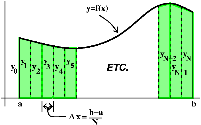 Putting it together
The picture attempts to illustrate what happens when a bunch of
trapezoids is used. Due to the scale of the picture and the thickness
of the lines, it is hard to see the error, but it is there. The error
is there because the graph is not made of line segments: it curves (in
fact, it curves, and somehow the amount the graph changes from being a
line is measured by the second derivative, which magically
appears below).
What does the trapezoid formula look like? Here:
[(Δx)/2](y0+y1)+[(Δx)/2](y1+y2)+[(Δx)/2](y2+y3)+...+[(Δx)/2](yN–1+yN)
If you notice, this can be reorganized a bit and this is done below.
Trapezoid Rule
Here is the reorganized formula, and an error estimate (getting this
error estimate is not as easy as the one before). The formula is
called the Trapezoid Rule.
Formula [(Δx)/2](y0+2y1+2y2+...+2yN–1+yN)
Error Less than
K2(b–a)3/(12N2) where K2
is some overestimate of |f´´(x)| on all of [a,b].
Here what is important is the N2 on the bottom, since that
gets larger much faster than N alone. Verification of the error
estimate takes two uses of MVT. I didn't do it in class and I won't do
it here.
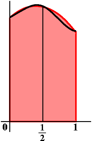 Ha: use three sample points, and parabolas!
I will write about this a little bit differently from what I did in
class. Go back to y=f(x) on [0,1], and let's use A+Bx+Cx2
where A and B and C are selected so that at 0 and 1/2 and 1 the values
will be f(0), f(1/2), and f(1). Because parabolas curve and
maybe most functions have graphs that curve also, we might hope that
the integral of the parabola is closer to the true value of the
integral of the function. Now
∫01A+Bx+Cx2dx=Ax+(B/2)x2+(C/3)x3|01=A+B/2+C/3.
Well, f(0) is A and f(1/2) is A+(B/2)+(C/4) and f(1) is A+B+C. Now one
needs some inspiration in order to write A+B/2+C/3 in terms of those
three quantities. Well, here is the inspiration. Suppose you take 4
times the value at 1/2: that's 4A+2B+C. Add on the values at 0 and at
1. The result is A+(4A+2B+C)+(A+B+C)=6A+3B+2C. (There are other ways
of guessing, ways which are more systematic, and allow
generalization, but I don't have time to show them to you: I am
sorry.) Now 6A+3B+2C happens to be 6 times the integral, so we should
divide f(0)+4f(1/2)+f(1) by 6. Sigh, really, this is not at all
clear!
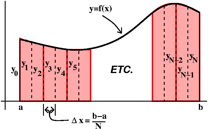 Simpson's Rule
I want to lift the formula from the [0,1] case and use it in general.
Let's "transport" the parabola setup to the more general picture,
piecewise. So what do we need? First, we need to assume that N is
even because we will be applying the parabola idea to pairs
of the "panels". O.k.: fine. But the width of the subinterval is
Δx, and this corresponds to ... what? In the interval case,
this corresponds to 1/2. So we should just divide by 3 here instead of
6. So this is what happens in the first few pairs of intervals:
1y0+4y1+1y2 gets multiplied by (Δx)/3.
1y2+4y3+1y4 gets multiplied by (Δx)/3.
1y4+4y5+1y6 gets multiplied by (Δx)/3.
· · ·
1yN–2+4yN–1+1yN gets multiplied by
(Δx)/3.
If you observe the "structure" of the formula, you can see what
happens. The 1 4 1 patterns overlap, and the "inside" 1's
become 2's. So this is Simpson's Rule:
Formula [(Δx)/3](1y0+4y1+2y2+4y3+2y4+...2yN–2+4yN–1+1yN)
Error Less than
K4(b–a)5/(180N4) where K4
is some overestimate of |f4(x)| on all of [a,b].
The implementation of Simpson's Rule is not much more work than the
Trapezoid Rule or the "Rectangular Rule": just keep a running total of
the odd and even heights inside the interval, multiply the odd
final total by 4 and the even final total by 2, add on the end
heights, and finish by multipling by a third of the interval
length. Seriously, that's not too much work, especially since
multiplications by 2 and 4 on a binary computer are just some shifts.
What happened to the error?
The fantastic thing is that the error is some number divided by
the fourth power of N. That's unexpected. I have gone through a
direct proof of the error formula. It is not pleasant, but it can be
done (there are some very clever proofs -- I only went through an
"elementary" proof). What is amazing is that there's an
N4 and not a cubic power. Why? Well, accidentally
(more or less!) the Simpson's Rule formula is valid for x3:
we're just lucky. What do I mean? Well, ∫01x3dx=1/4, certainly (since
∫x3dx=[x4/4]+C). And the idea was that we
should compute f(0)+4f(1/2)+f(1) divided by 6. Well, if
f(x)=x3, then f(0)=0, f(1/2)=1/8 and f(1)=1. So
f(0)+4f(1/2)+f(1)=0+4(1/8)+1=3/2. When we divide that by 6 we get
(3/2)/6=1/4: the correct answer! So we gain another power of accuracy,
and the error formula is even smaller.
|
Some numerical evidence
I computed (well, a machine did, at my direction!) approximations to
two examples and wrote the results on the board. One was
∫12[1/x]dx=ln(x)]12=ln(2)=ln(1)=ln(2)–0=ln(2),
which I "know". The other is
∫01[4/{1+x2}]dx=4 arctan(x)]01=4 arctan(1)–4 arctan(0)=4(Π/4)–4(0)=Π,
something else I presumably know. Here are the results, with the three
different rules and with a varying number of pieces in the partition.
| ∫12(1/x) dx, approximately 0.6931471806 (ln 2) |
|---|
| n= | Left Hand Rule | Trapezoid Rule | Simpson's Rule |
|---|
10
100
1,000
10,000
100,000 |
0.7187714032
0.6956534302
0.6933972431
0.6931721811
0.6931496806 |
0.6937714035
0.6931534305
0.6931472430
0.6931471810
|
0.6931473748
0.6931471808
0.6931471803
|
|
| ∫01(4/{1+x2}) dx, approximately 3.141592654 (Π) |
|---|
| n= | Left Hand Rule | Trapezoid Rule | Simpson's Rule |
|---|
10
100
1,000
10,000
100,000 |
3.239925989
3.151575986
3.142592487
3.141692652
3.141602654 |
3.139925989
3.141575988
3.142592487
3.141592652
|
3.141592652
3.141592653
|
Things to think about
Although in theory any one of these computational schemes can give you
any accuracy desired, in practice there are other considerations.
First, you can worry about the amount of computational time. Function
evaluations take time on real machines. The lowest row (n=100,000)
took about half a minute. Second, numbers are represented on real
machines using floating point techniques, and arithmetic using
floating point numbers passes along and increases errors. That is,
sort of, there is "dirt" in the lowest digit or two, and the more
things you do, the more the dirt is spread around. Therefore reducing
the number of divisions, multiplications, etc. is definitely a good
idea. For both of these reasons, and some others, the table should
convince you that the Trapezoid Rule and, especially, Simpson's Rule,
are worthwhile. They require almost the same amount of computation as
simple rectangles at each level, just a little more bookkeeping. But
the N2 and especially the N4 "downstairs" in the
error estimates make these Rules worthwhile.
What you should know ...
The textbook discusses the Midpoint Rule in addition to the Trapezoid
Rule and Simpson's Rule. You should know about these three, and have
some feeling for how the error estimates work. Please note that there
are calculator
programs available for all three of them which work on some of the
more common graphing calculators. This may help you with some of the
textbook homework problems.
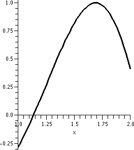 A specific example, with details
I will try to give more details with this example. I should have done
something like this in class. My function will be
f(x)=sin(x2+5) and the interval will be [1,2]: those x's
with 1≤x≤2. A graph of the function on this interval is to the
right. There is no way to directly apply FTC in the
computation of this integral using familiar functions.
What do you think is the value of
&int12sin(x2+5)dx? Well, there's a
little chunk of negative on the left-hand side, and the rest of the
graph sort of is almost a triangle. It is a bit bigger than the
triangle on the right, but the left negative chunk will bring the
number down. If I had to "guess", I would say that the integral is
about (1/2)(1)(1) (area of a triangle with base 1 and height 1). A
sophisticated numerical integration program reports that the value is
0.5651369238 (indeed!).
I want to try to estimate the value using the three methods mentioned
in this lecture. I will also try to estimate the accuracy using the
stated error bounds. I will use N=10. This means there will be N+1=11 y-values:
y0=f(1), y1=f(1.1), y2=f(1.2),
y3=f(1.3), y4=f(1.4), y5=f(1.5),
y6=f(1.6), y7=f(1.7), y8=f(1.8),
y9=f(1.9), and y10=f(2). For example,
y7=f(1.7)=0.9993514088 (look at the picture and see that
the value at x=1.7 is near the top!). Also,
(b–a)/N=(2–1)/10=.1 and this is Δx.
Level 0, rectangles sampled on the left
Approximate value
So here we want
Δx(y0+y1+y2+y3+y4+y5+y6+y7+y8+y9). If
"you" do all the arithmetic (I had a silicon friend do it)
0.5259155121 is the result.
Error analysis
Since f(x)=sin(x2+5), we get
f´(x)=cos(x2+5)2x. How big can this get on [1,2]?
Well, laziness is important. Look, the biggest that
|cos(x2+5)| can be is 1. The biggest that |2x| can be on
[1,2] is 4. So I think that one good overestimate for K1 is
4. Certainly b–a=1, and therefore we know
K1(b–a)2/N=(4)(12)/10=.4 is an upper
bound for the error.
Comparison of theory and the approximation we got
Well, 0.5651369238–0.5259155121 is about .04, so, in fact, the result
is considerably more accurate than the theoretical bound. If
you look at the picture, you may be able to see why. To the left of
the max, the rectangles are below the curve, and to the right of the
max, they are above the curve. So there is nice cancellation. We are
fortunate.
Level 1, Trapezoid Rule
Approximate value
So here we want
(Δx/2)(y0+2[y1+y2+y3+y4+y5+y6+y7+y8+y9]+y10). My silicon pal reports that the result is
0.5604922111 which is nice, I guess.
Error analysis
We need the second derivative. Since
f´(x)=cos(x2+5)2x, we get
f´´(x)=–sin(x2+5)(2x)(2x)+cos(x2+5)2. Now
I will be even lazier, and just analyze each part separately. Also, I
am interested in absolute values, so I will discard any minus signs. I
just want a lazy estimate of K2. What about
|–sin(x2+5)|? Overestimate by 1. And |(2x)(2x)| on [1,2]:
overestimate by 16. And |cos(x2+5)2| is overestimated by
2. Put these all together and I think that K2 is overestimated by
18. Then K2(b–a)3/(12N2) becomes
(18)(13)/[12(10)2] and this is .015, our error estimate.
Comparison of theory and the approximation we got
True value minus this approximation is 0.5651369238–0.5604922111
and this is about .005, which is again less than our estimate. The
estimate we got, by the way, is how people actually do this in
practice. Generally no one wants to spend time getting the absolutely
best possible error estimate -- we just want an
approximation. But one caution: your approximation should
always be an overestimate of the error since you want your result (the
result you report, with "error bars") to be reliable.
Level 2, Simpson's Rule
Approximate value
The weird 1-4-1 pattern needs to appear, with the inside 1's doubled:
very strange. Therefore we want
(Δx/3)(y0+4[y1+y3+y5+y7+y9]+2[y2+y4+y6+y8]+y10). Electrons
again move and compute and 0.5651387559 is the reported result.
Error analysis
This will certainly be painful. We need the fourth
derivative. Start with
f´´(x)=–sin(x2+5)(2x)(2x)+cos(x2+5)2
and then get
f(3)(x)=–cos(x2+5)(2x)3–sin(x2+5)(8x)–sin(x2+5)(2x)2. Let
me clean this up a bit, and instead write
f(3)(x)=–cos(x2+5)(8x3)–sin(x2+5)(12x). Now
another derivative:
f(4)(x)=sin(x2+5)(2x)(8x3)–cos(x2+5)(24x2)–cos(x2+5)(2x)(12x)–sin(x2+5)(12). I
am trying here not to cheat and use any shortcuts. There is a bit of
"simplification" which can be done:
f(4)(x)=sin(x2+5)(16x4)–cos(x2+5)(48x2)–sin(x2+5)(12). Now
estimate. Well, all of the sines and cosines with + or – will be
estimated by 1. And 16x4 on [1,2] is at most
16·24=162=256, while 48x2 is
overestimated by 48·22=192 and K4 is
overestimated by 256+192+12=460. The error overestimate will be
K4(b–a)5/(180N4)=460(15)/[180(104)]),
wow. In decimals, this is .000256. So the Simpson's Rule
approximation is at least this accurate.
Comparison of theory and the approximation we got
True value minus the approximation is 0.5651369238–0.5651387559,
about .000002, so the Simpson's Rule approximation is actually closer
by a factor of 100 times to the true value. This is o.k. to me. But I
don't know why it is so much more accurate (that is, I can't give a
heuristic reason): sorry.
So I went to my faithful companion, Maple, and had it compute the fourth
derivative, which I really did "by hand" above. And my/our computation
was correct. Then I asked for a graph on [1,2]. Not so oddly there is
some cancellation. The analysis above to get some value for
K4 assumes there is no cancellation. And the K4
suggested by the graph is about 47.2 compared to 460 above. So one
order of magnitude difference in the error observed is explained. But
I still can't understand why the result is 10 times better than
expected: sorry.
|
QotD
This would have been the QotD if I had time, darn it!
| Time | Rate, in gal/hr |
|---|
| 1:00 | 50 |
| 2:00 | 70 |
| 3:00 | 35 |
| 4:00 | 60 |
| 5:00 | 40 |
Here is some data ("flow rates" measured at various times) shown in
the table to the right. Of course this would be for toxic waste or
something like that. Sigh. Then the definite integral would measure
the total flow: flow rate multiplied by time interval, so the units
work out o.k. (hours times gallons per hour). I would have liked
approximations for the definite integral.
- A (left) "Rectangular Rule" approximation for the flow (in
gallons, which is what you get by integrating gals/hr over time: the
flow rate integrated gives you the net flow) is, with
Δx=1:
(1)(50+70+35+60).
- A Trapezoid Rule estimate is, with
Δx=1:
(1/2)(50+2·70+2·35+2·60+40).
- A Simpson's Rule estimate is, with
Δx=1:
(1/3)(50+4·70+2·35+4·60+40).
If you've gotta have the numbers (?) I think they are 215 and
210 and 226.6666...
| Wednesday,
September 9 | (Lecture #3) |
|---|
Problem from the textbook
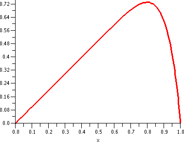 Here is problem 48 (must be very
difficult!) from section 6.4.
Use the Shell or Disk Method (whichever is easier) to
compute the volume of the solid obtained by rotating the region shown
(y=x–x12) about
(a) the x-axis (b) the y-axis.
Let's solve (a): we do it dx and get
∫LeftRightΠ(Radius)2dx=∫x=0x=1Π(x–x12)2dx=Π∫01x2–2x13+x24dx=Π([x3/3]–2[x14/14]+[x25/25])|01=Π([1/3]–[2/14]+[1/25]).
Now for (b). If I wanted to do this dy, I would need to solve
y=x–x12 for x. I don't know a formula for this, and NO ONE
ELSE IN THE WORLD DOES. This would not be a feasible method. But dx
things are easy (thin shells). Here we go:
∫LeftRight2Π(Radius)(Height)dx=∫012Π(x)(x–x12)dx=2Π∫01(x2–x13)dx=2Π([x3/3]–[x14/14])|01=2Π([1/3]–[1/14]).
Why is this problem 48? For many people the "natural" way to compute
the volume for part b) is dy, and get the rotated dy strip as an
object which is dy thick and which has cross-sectional area equal to
the area between two concentric circles. This is all fine, but getting
useful formulas for the two radiuses (radii?) involved is not
possible. So this problem is difficult for psychological
reasons!
Work
which is physics which is something I know little about. I have been
told that Work=Force·Distance. Also I have been told that units
matter, and the most generally used units for Distance, Force, and
Work are meters, newtons, and joules. I will use as my units feet,
pounds, and foot-pounds. Sigh. So lifting 10 pounds for 5 feet does 50
foot-pounds of work. Huh. The only thing wrong is that the
abbreviation for pound is lb.
 Pulling a chain up a cliff
I have an iron chain which weighs 3 pounds per foot and is 100 feet
long. It hangs from the edge of a tall cliff. How much work is
required to pull the chain to the top of the cliff?
Here's a picture of the chain. (Drawing the pictures is the fun part
for me.) We can imagine the chain's length being broken up into tiny
pieces, and then we would need to lift the pieces up the cliff. Let's
see: suppose we have a piece which is x feet from the top of the
cliff, and a tiny piece of length dx is imagined there. Then the
weight of that tiny piece is 3 dx (the 3 above is actually a sort
of linear density). To lift just that piece to the top of the cliff
needs x·3 dx amount of work. But the whole chain is made
up of these pieces, and so we need to add up this amount of work, and
(due to the way I set this up) we should take the integral from the
top (x=0) to the bottom (x=100) of the chain. This will get the total
work:
∫01003x dx=(3/2)x2|0100=(3/2)(100)2.
 Hooke's Law
I gave a fantastic demonstration of Hooke's Law, using
specially obtained titanium (?) wire hangers and specially obtained
elasticium (?) bands on a specially crafted teak rod. Maybe now I can
take a $10,000 tax deduction (doubtful). Anyway, an approximate
demonstration of Hooke's Law was given. Hooke
was a strange person.
It is somewhat interesting that validity of Hooke's Law can be shown
even with a rather crude setup.
Springs
Many real world springs obey Hooke's Law over "a portion of their
elastic range". This means that the distortion of the spring from its
equilibrium length is in a direction opposite to the impressed force
and has length directly proportional to the force. This is, more or
less, "F=kx", where F is the force and x is the distortion from
equilibrium and k is a constant, frequently called the spring
constant. So twice the weight on a spring will distort it twice as
much, but you probably should not assume the same for, say, ten
thousand times as much weight. Here's a typical Hooke's law/work
problem.
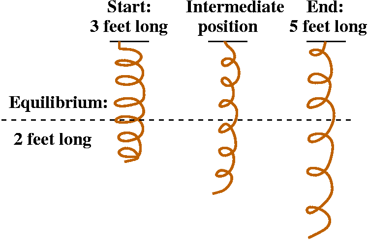 Pulling a spring
In equilibrium a spring is 2 feet long. A weight of 10 pounds
stretches it to 2.5 feet. How much work is needed to stretch the
spring from 3 feet long to 5 feet long?
Since 10 pounds changes the length of a spring by .5 feet, we know
that 10=k(.5) so that the spring constant, k, must be 20. Now consider
the various stages of the spring as it goes from the start position
(when the length is 3 and the distortion of 1) to the end position
(when the length is 5 and the distortion is 3). I'll call the
distortion, x. Perhaps we could consider an intermediate position. If
we pull the spring just a little bit more (change the length from x to
x+dx) we won't change the force very much. The force needed in that
intermediate position is 20x. The additional distance we're stretching
the spring is dx, so the "piece of work" we're doing is
20x dx. To get the total work we need to add up the pieces of
work from 3 feet long (when x=1) to 5 feet long (when x=3).
∫1320x dx=10x2|13=10(32)–10(12).
Caution When I do these problems, I
sometimes make an "easy mistake". I confuse the spring length with the
distortion from equilibrium. Hooke's law applies to the distortion, so
that is what must be considered.
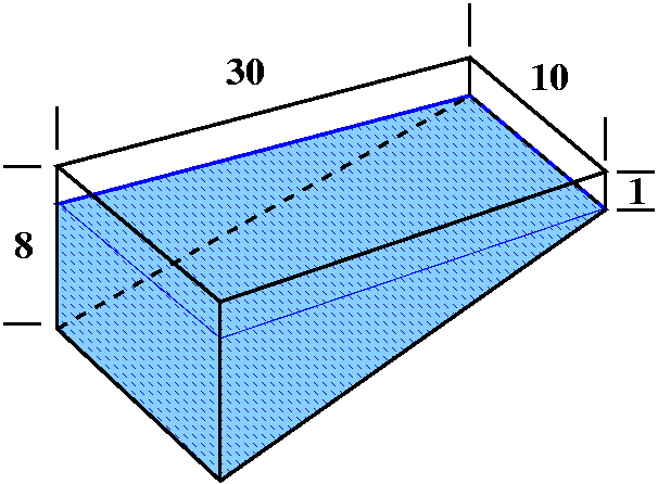 Emptying a pool
A pool has a rectangular top, 10 feet by 30 feet. The pool is 1 foot
deep at one of the edges which is 10 feet long, and is 8 feet deep at
the other edge which is 10 feet long. The depth varies linearly
between these edges. The pool is filled with water but the top of the
water level is 1 foot below the top of the pool. How much work is
needed to pump out the water in the pool (that is, to the top of the
pool?).
An oblique view of the pool is shown to the right. I hope that
this picture corresponds to what your view of the description in words
above. We need to raise the water to the top of the pool. To do this,
we need some information about the force needed (the weight of the
water).
The density of
water is about 62.5 pounds per cubic foot. Generally, of course,
stuff near the bottom compresses, but it turns out that water has
rather low compressibility
and we can accept the 62.5 as valid for all of the water in the pool.
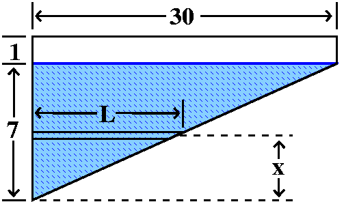 Although the lovely picture above pleases me (artistically!), a more
reasonable view might be sideways. I will put the origin of a
coordinate system for depth at the bottom of the pool (certainly there
may be one or two other reasonable places to put it). Then I will look
at a typical intermediate slice of the water volume at height x from
the bottom of the pool. The slice will have thickness dx. The reason
to look at this is that all of the water in that slice will need to be
lifted the same distance to the top of the pool. So this method of
organizing the computation allows me to put the distance into one part
of the problem, and then concentrate on the force (the weight of the
slice) in another part of the problem. But now we need to think about
the volume of the slice. It is dx thick, and I hope you can see that
the cross-section of the slice is a rectangle. It goes entirely across
the 10 foot width of the pool, and what varies in the slice is the
length, which I labeled L in the diagram. Similar triangles tell me
that L/x=30/7 so that L=(30/7)x. The volume of a slice is
(10)(30/7)x dx, so that the weight of a slice is
(62.5)(10)(30/7)x dx. This slice needs to be lifted to the top
of the pool (not just the top of the water!) and this distance is
1+(7–x)=8–x (I wrote it this way to emphasize that 7–x is the distance
to the top of the water, and 1 more foot to get to the top of the
pool). So the amount of work needed is (8–x)(62.5)(10)(30/7)x dx. To
get the total work I need to add up the work from the bottom of the
water (x=0) to the top of the water (x=7):
∫07(8–x)(62.5)(10)(30/7)x dx=(62.5)(10)(30/7)∫078x–x2dx=(62.5)(10)(30/7)
(4x2–x3/3)|07=(62.5)(10)(30/7)(4(72)–73/3).
The QotD was the computation of this integral.
Some comments on solutions of the work problems
The methods of solution are reasonable and the selection of problems
that I showed you was carefully structured.
- In the the
chain problem, the force was constant (3dx) and the distance varied.
- In the
spring problem, the distance was constant (dx!) and the force
varied.
- In the third problem, both the distance (8–x) and the force
(the slice's weight) varied, and the problem solution was organized the
problem so that we took advantage of the geometry.
| Wednesday,
September 2 | (Lecture #2) |
|---|
Surviving math lectures
Here is some advice. It is really well-intentioned.
- Try to stay awake. (80 minutes is a long time. Math can be
dreary and intensely difficult to engage with.
- Take notes. The idea is that at least you would do
something and not sit there almost paralyzed. The "default"
option in math lectures is to copy anything the instructor writes on
the board. Usually that won't include very bad jokes and will include
mostly what is essential. You may want to add your own
comments. Taking notes and thinking and listening turns out to be
difficult in practice.
- Ask questions. We have a relatively small class, and this is the
only true luxury of the H sections. If you don't understand something,
probably half the people listening don't also. The instructor most
likely can't read your mind and can't perceive the lack of
communication, so do something nice for the "community": ask about
it. The darn instructor should be able to explain things, and, if not,
might respectfully postpone a response until later in the class or,
rarely, out of class. But you should try. This helps.
Another volume by slicing
Suppose we have a solid whose base is the same region we discussed
last time (bounded by y=4x and y=x3 in the first quadrant),
so that the cross-sections or slices of the solid which are parallel
to the y-axis and perpendicular to the xy-plane are half-discs
(semicircles) with diameters in the xy-plane. What does the solid look
like, and what is its volume?
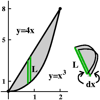 Here of course we will slice the solid dx. The cross-sectional area is
the area of half of a circle whose diameter is L. Well, the area of a
whole circle with radius Π is Π·r2. Here r is
(1/2)L, so that the cross-sectional area is
(1/2)Π[(1/2)L]2. Repeating: the first 1/2 is because we
have half of the area of a circle, and the second 1/2, inside the
parentheses, is because we are changing diameter into radius. Here the
setup is dx. The limits of integration look back to the first
computation of the area, so that x=0 is the lower limit and x=2 is the
upper limit. L is what I called Height then, so
L=4x–x3. What is the volume of the solid? Here we
go. Notice that the (Π/8) factor comes from Π(1/2)(1/2)2
pulled out of the integral (we can do that with multiplicative
factors!).
(Π/8)∫02(4x–x3)2dx=
(Π/8)∫0216x2–8x4+x6dx=(Π/8)([16/3]x3–[8/5]x5+[1/7]x7|02=(Π/8)([16/3]23–[8/5]25+[1/7]27–0
Again, this is the way I would leave this answer, please please please!!!. If you are a
weirdo, and need "precision" then the exact value is
Π([128]/[105]). I don't know why there is a coincidence with the
last computation done in the first class. I didn't plan on it. Sigh.
Definition of the average value of a function
The average value or mean value of a function f(x)
defined on an interval [a,b] is
∫abf(x) dx)/(b–a).
I'll discuss why this definition is reasonable but first a very simple
example.
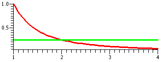 Example
Let's compute the average value of 1/x2 on [1,4]. So:
∫14(1/x2)dx=–1/x]14=–1/4–(–1/1)=3/4. (That's
because 1/x2 is x–2 which has antiderivative
{1/(–1)}x–1=–1/x. The average value is 3/4 divided by
4–1=3, so the average value is 1/4.
To the right is a graph of y=1/x2 on [1,4] together with a
horizontal line, y=1/4, the average value. Does it "look" right? I
hope so.
A continuous function on an interval and its average value
The average line does intersect the curve, though, always, if
the function is continuous. This is true because a continuous
function, f, on an interval [a,b] has a max, M, and a min, m, and its
integral must be between M(b–a) and m(b–a) so the average value
(divide by b–a) must be between M and m. Then the Intermediate Value
Theorem guarantees that y=f(x) must have this value at least once
somewhere in the interval.
Samples and sample means
If you model a physical process (or a computer algorithm) by f(x) for
certain values of x, say in [a,b], you might be interested in checking
the outputs or the running time or ... lots of things. So you might
sample the function f(x) on [a,b] a finite number of times:
x1, x2, ..., xn. Then you'd get
results f(x1), f(x2), ..., f(xn). You
might want to analyze these results statistically and hope that the
information you get would represent, somehow, information about "all"
of the values of f(x) on [a,b]. The average of these n outputs is
called the sample mean.
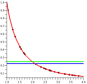 An example
Maple has a fairly good "random" number
generator. That is, the properties of the generator are known and have
been investigated systematically, and they satisfy many of the
statistical criteria that are desired for randomness. I asked for 30
random numbers between 1 and 4. The list began with 1.198304612 and
continued with 1.640439652 and then with 3.984266209 ... (27 more
numbers like this!). Then I computed the mean of the values of
f(x)=1/x2 for these 30 numbers. This sample mean was
0.2241511003. Remember, the average value for f(x) on [1,4] is 1/4, or
.25. The picture to the right shows a graph of 1/x2 on
[1,4], the 30 points created, and two lines. The top line is the
average value of 1/x2 on the interval (y=.25) and the lower
line is y=the sample mean. Please realize that the picture has been
distorted (the curve previously shown is correct) so that you can see
the two lines and the sample points more clearly.
|
Random samples and what can be hoped ...
If we take many, many samples on [a,b], we can hope (random? What does
"random" mean?) that these samples are distributed fairly evenly over
the interval. So then look at this:
 The sample mean        Multiply top and bottom by b–a
                         and rearrange algebraically
f(x1)+f(x2)+...+f(xn)     f(x1)+f(x2)+...+f(xn) (b–a)
--------------------  =  ---------------------·----- =
          n                      n             (b–a)

f(x1)·[(b–a)/n]+f(x2)·[(b–a)/n]+...+f(xn)·[(b–a)/n]
--------------------------------------------------
                     b–a
If you now look closely at the top, I hope that you can "see" a Riemann
sum for f on [a,b]: well, at least you should see values of f at sample points, and the length of a subinterval of [a,b] when [a,b] is split up into n
equal subintervals. We can hope that almost the sample points are in
the correct subinterval.
Connection between sample means and average value
It turns out that, if the sample points are chosen uniformly at
random over the interval [a,b], then the sample means will almost
always → the average value of the function (as defined above, with
the definite integral). To actually verify this takes some effort
because you need to understand what random and uniform and ... please
learn some probability and statistics.
Folding back on itself: how to approximate an integral
The previous result is true, and it has been used in very cute
reversed fashion which you may find difficult to believe. One can
compute sample means and then use the sample means to estimate the
definite integral. That is, if you wanted to know the value of
∫abf(x) dx numerically, approximately,
take a large number of samples of f(x) in the interval [a,b]
(uniformly, randomly) and take their average. Multiply the result by
the length of the interval, b–a. The result is an approximation
to the value of the integral. This is known as the Monte Carlo
method for estimating the value of the definite integral (really!)
because it seems to use gambling ideas (random numbers).
Another example
Maple has a fairly efficient (fast and
satisfies some well-known criteria for randomness) random number
"generator". I used it to try to compute the integral of x3
over the interval [5,8]. The "true value" of this integral is
867.95. Here are Monte Carlo approximations for specific "flips" (?)
or choices of random points in the interval. What I asked Maple to do is the following: select some "random"
numbers between 5 and 8, say x1, x2, ...,
xn. Then compute this sum:
x13+x23+...xn3.
Then divide this by n, and multiply by 3, the length of the
interval. The results of this experiment are below. Please realize
that if I ran this experiment another time I would likely get
different results (!). The value of the integral doesn't change, but
the approximation does: very strange.
| # of points | Reported approximation |
|---|
| 10 | 1007.29154 |
| 100 | 815.78669
|
| 1,000 | 850.26269 |
| 10,000 | 868.39938 |
| 100,000 | 867.07575 |
| 1,000,000 | 867.77362 |
| 10,000,000 | 867.66869 |
Please notice that the results "seem" to be getting closer to the true
value, but the approach is not very systematic. Actually the last
answer is more distant than the preceding one. (A possible reason is
accumulated inaccuracy because of the large numbers of floating point
arithmetic operations which are needed.) Such a technique is called a
Monte Carlo method because of its dependence on randomness
(Monte Carlo↔gambling/casino↔random).
I'd use Monte Carlo
methods only if other numerical or analytic approaches seem to be
inadvisable. We will see later in the course many methods for
computation of integrals.
Here is further information about the Monte Carlo
method.
Getting efficient ways of generating random numbers (really,
pseudo-random because they are obtained in various
deterministic ways) is very important when using this method. Heck,
this is also important in other applications, such as cryptography.
|
Solids of revolution
A collection of solid objects with central symmetry are known as
solids of revolution. They occur often enough in applications
that we should spend some time discussing them. Below are pictures of
some of these solids. Revolving a rectangle around one of its sides
gives a cylinder. Revolving a right triangle around one of its legs
gives a cone. Revolving a semicircle around its diameter gives a
sphere. Revolving a circle around an external line gives a torus (a
doughnut).
Volume of a right circular cone
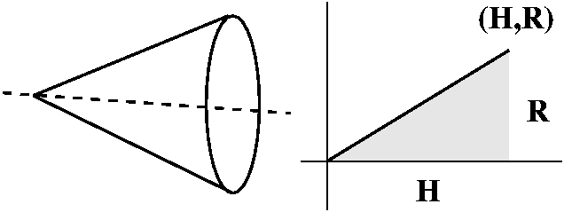 Formulas for the volumes of all of these solids can be gotten using
the methods of today's class. I'll just do one, the cone. Really this
is called a right circular cone, "circular" because the slices of
the solid perpendicular to its axis of symmetry are circles, and
"right" because the axis of symmetry is perpendicular to the base. The
textbook formula for the volume of a cone with base radius R and
height H is (Π/3)R2H. We can get this cone by revolving
the area under a line segment going from (0,0) to (H,R) around the x-axis.
The slope of this line is R/H, and its equation is y=(R/H)x.
If we slice perpendicular to the x-axis, by slices which are
perpendicular to the x-axis, we get (approximately!) a bunch of
circular discs which are dx thick and which have radius (R/H)x. So dV,
a piece of the volume, is Π[(R/H)x]2dx. The total volume
is the sum of the dV's added up from x=0 to x=R. So the volume is
∫x=0x=RΠ[(R/H)x]2dx=Π(R2/H2)∫x=0x=Rx2dx=Π(R2/H2)x3/3]x=0x=R=Π(R2/H2)R3/3=(Π/3)R2H
The final result is the formula which everyone "knows". The first
equality is true because we can pull multiplicative constants out of
integrals, and then the next is a simple use of FTC.
Computing the volume another way
The method about is called circular discs or coins. Let me now show
you a different way. Let's slice the region dy: by many horizontal
lines very close together (dy apart). Now take one of the rectangles
which is dy high, and revolve it around the x-axis. The result is
what's called a thin shell. We can cut it with magic scissors (?) and
flatten it out. Yes, there will be some distortion of volume, but some
volume is expanded and some is compressed, and it turns out that the
effects cancel. The result is just about a rectangular
parellelopiped. Its volume with be the product of the lengths of the
edges. One edge is dy, and another is 2Πy, the circumference of the
circle which the thin rectangle describes. What about the last edge?
It is the distance between y=(R/H)x (or x=(H/R)y) and x=H. So this
distance is R–(H/R)y. This chunk of volume, dV, is
2Πy[H–(H/R)y]dy. We need to add this up from bottom (y=0) to top,
(y=R). Here we go:
∫y=0y=R2Πy[H–(H/R)y]dy=
2Π∫y=0y=R[Hy–(H/R)y2]dy=
2Π∫y=0y=R
[Hy2/2–(H/R)y3/3]]y=0y=R=
2Π[H·R2/2–(H/R)R3/3]=
2ΠHR2[(1/2)–(1/3)}=
(Π/3)HR2
So we get the same result (thank goodness!).
I was asked the extremely reasonable question whether learning another
way to compute the volume of a solid of revolution was
reasonable. Well, examples show that sometimes one approach can be
completed effective, and sometimes, the other. The more methods you
know, the better. I really believe this. Here's an example.
 The Cauchy distribution
To the right is a graph of f(x)=1/(1+x2). This function is
alway positive, and it is even (f(x)=f(–x)). When |x| is large (either
positive or negative) the values of the function →0. The curve is
sometimes called the Cauchy distribution. It is a very
important object in statistics and physics, and is what's known as a
"fat-tailed" distribution (really!). General information about it can
be found here and
here,
and there is a neat applet involving the Cauchy distribution here.
Revolving a chunk around the y-axis
Suppose we want to revolve f(x)=1/(1+x2) from 0 to 1 around
the y-axis. If you wanted to use "discs" you would need to solve for x
as a function of y. So y=1/(1+x2) would give
x=sqrt(1-{1/y}) but this is not the only problem. In fact, from the y
point of view, this formula would only be valid from 1/2 to 1. So the
volume would need two integrals. The computation can be done
this way, and I would not want to prevent you from doing it. But
... the shell method is much easier.
So let me integrate dx and use the thin shell method. The height of
the shell is 1/(1+x2), and it is a distance of x from the
y-axis making the circumference 2Πx, and its thickness is dx. The
definite integral we must compute is this:
∫x=0x=12Π[x/(1+x2)]dx.
The QotD
Compute this definite integral. There were some hints offered:
u and substitute and ...
Indeed, if u=1+x2, then du=2x dx, so
(1/2)du=x dx, and [x/(1+x2)]dx=(1/2)du/u. This
antidifferentiates to (1/2)ln(u) or (1/2)ln(1+x2). Now
don't forget the 2Π! So we need
(2Π)(1/2)ln(1+x2)]x=0x=1=Πln(2)–Πln(1)=Πln(2).
| Wednesday,
September 2 | (Lecture #1) |
|---|
Due on Thursday (tomorrow): solutions of 6.1: 16 and 26.
There was some informal discussion of the instructor, the students,
and the course. And even 2009 AB6 was mentioned.
What do you need to know?
Math 152 is the second semester of the three semester calculus
sequence which is given for students who really need to know
calculus (or who are quite curious!). In many respects it is the most
technical, most computational of the three semesters. I personally
think it has many fewer big ideas and lots of computational tricks. So
what should you know to take this course?
- You need to know quite a bit about specific functions. You should
know about the derivatives and integrals and domains and ranges and
graphs of powers (xb), exponential (ex),
logarithm (ln x), trig functions (certainly sine, cosine, tangent,
sometimes secant), inverse trig functions (certainly arcsine and
arctangent, and sometimes arcsecant).
Some poor engineering and physics majors may need to learn about the
hyperbolic functions, so I will describe them later this semester.
- The most important results to remember from earlier calculus are
the Fundamental Theorem of Calculus (FTC) and the Mean Value
Theorem (MVT). By FTC I mean a bunch of ideas, something like:
- The definite integral is defined to be a limit of a
sum, and the sum is gotten in the following strange way: slice up the
domain interval into many subintervals; multiply function values in
each subinterval by the length of that subinterval; add up the
products. Amazingly, that process gets close to one specific number
(converges in more precise language) as the largest length of
the subintervals gets shorter. The specific limiting value is the
definite integral.
- One way to compute the definite integral is to find an
antiderivative of the integrand (the function whose values you're
looking at), and then taking the difference of that function's values.
- The definite integral itself, when considered with a variable
upper bound, has derivative equal to the integrand function.
MVT is a slightly more slippery idea, because it is presented as a
fact about secant lines and tangent lines (the average value
[difference of the function values at the endpoints divided by the
length of the interval] is equal to at least one instantaneous rate of
change [derivative] in the interval). In fact, the way MVT is used
computationally is as part of an equation, so
f(a+h)=f(a)+f´(c)h etc.. We will relearn
MVT and extend it enormously later this semester.
- You should also know about how to use simple substitution to find
antiderivatives. This semester we'll discuss more complicated
strategies.
What this course is about
Math 152 is quite technical. The principle excuse for the
technicality is that if you will have a career in science or
engineering, the methods of the course are assumed to be part of the
background of everyone. The course asks students to do some
hand computation which can be very elaborate. In most workplaces, this
computation will likely be strongly assisted by Maple or Mathematica or Matlab. (I use Maple myself but the others have similar
qualities.) The excuse for having students learn to compute by hand is
that they should then have some feeling for what strategies are useful
and for what the "shape" of the answers is like.
More precisely (about as precise as I can be at this stage) here is
what the course is about:
Part 1: some uses of the definite integral
Definite integrals are used to compute lots and lots of quantities:
areas, volumes, masses, moments, pressures, ... hundreds of other
things you will learn about.
I'll use this background color for material I didn't have time to do
in class.
A friend of mine wrote in a recently
published book that "This method of finding areas
is paradigmatic for an entire class of problems in which one is
multiplying two quantities such as
- area = height x width,
- volume = cross-sectional area x width,
- moment = mass x distance,
- work = force x distance,
- distance = speed x time, or
- velocity = acceleration x time,
where the value of the first quantity can vary as the second quantity
increases." He is a great scholar, and uses words
precisely. The word "paradigm" means "an example or pattern." The
definite integral can be used to compute or approximate many
quantities (many more than are in the list just given). That's the
real power of calculus. |
Very few of you will compute many areas professionally (or, actually,
any areas professionally!). But I am fairly sure that almost
all of you will need to investigate and compute many definite
integrals. So initially we will consider some simple uses of definite
integrals. All of the quantities will be computed by the sequence of
ideas:
Chop up → approximate → add → take limits
which turns out to be wonderfully useful.
Part 2: computing definite integrals
Once you have the creature (a definite integral), what is the
vale of the integral?
38.5? Π/sqrt(2)? We need some methods.
- Some simple numerical methods
In many cases,
all that can be obtained is some approximation to the true value. And
that is frequently good enough. Although, again, it is likely most
students will just use "canned" programs or routines created by other
people, students should have some basic idea of what's going
on. Numerical routines can easily give incorrect or misleading
answers.
- "Well-known" symbolic tricks
For example, in 151 we showed
some substitutions were found which allow
antidifferentiation and then evaluation of the definite integral via
FTC. In fact,
human beings, using substitution, can find antiderivatives that
TI-89's and even Maple and Mathematica can't! There are some other
"standard" methods which students should know about. While they are
implemented by computers, knowing these methods also gives insight into
the behavior of the integrals (how big, how small, what to
expect). There's lots of algebraic computation needed here.
- Geometric methods
Here we learn how to use pictures (!)
to get information about integrals. The context in which this is
presented is solutions of differential equations. The pictures can
sometimes allow predictions of asymptotic behavior (what happens to
competing species over a long time, or what happens in a solution of
various chemicals with several reactions going on) which would be
difficult or impossible to predict numerically or algebraically. These
methods are much more useful than students initially guess.
Part 3: how to compute values of functions
Many functions are used to model physical situations. They can be very
complicated. A result called Taylor's Theorem can be used to
approximate these intricate and weird (!!) functions. Taylor's Theorem
is a generalization of MVT, and it shows how to approximate functions
by polynomials. Polynomials are easy to compute. The type of
approximation leads rapidly to a new way of describing functions,
using what are called infinite series, especially a specific
type of these called power series. These descriptions, which
again have lots of intricate algebra involved, will be studied for a
big chunk of the semester.
That's the plan of the course. There are a few minor additional
topics, but please take a look at the syllabus. It will give you a
good idea of where we are headed.
How do we teach it?
There are two lectures each week. The lecturer is correct 72.6% of the
time, and students should point out the almost inevitable exxors. The
diary may help. There is an additional meeting each week. Most of
those meetings will have most of their time devoted to
workshops. Small groups of students will investigate calculus
problems. Students will then be asked to do writeups of some problems. I may
also ask students to do oral presentations of problem solutions. The
workshops and writeups are an extremely important and useful part of
your technical education. You also will had in textbook problems at
the workshop.
Attendence is important. Almost all the students who have poor
attendence do badly on exams and tend to get low course grades. This
does not always happen, and certainly (the other way around!) there
are students who come to class faithfully and are not extremely
successful, but there is very good correlation between class
attendance and learning the material so that mastery can be displayed
on exams.
 Do all of the homework!
Work with other students!
Read the textbook!
Let's begin
We will compute the area in the plane enclosed by y=x3 and
the line segment which joins (0,0) and (2,8). The region is shown to
the right. The points (0,0) and (2,8) are on y=x3, and the
region is bounded by the line y=4x and the cubic curve. (This is not
supposed to be difficult to see!).
First method
 We slice the area by lines parallel to the y-axis. I think of the
lines as dx apart. The region is chopped up into things which
are almost rectangles, and the area of each piece is going to
be HEIGHT·dx. We will get a good approximation to the total
area by taking the Sum of the areas of
these almost rectangular pieces. Of course what I mean by "Sum" is a definite integral, because that includes
a limiting process which makes increases the accuracy of the
approximations. So in this setup, we will have ∫LeftRightHeight dx. We add up the
slices from the left to the right of the region. Here we have slices
which are dx thick, and we should try to write everything in terms of
x. Let's see: the Left and Right are easy enough, because the
left-most point of the region occurs when x=0, and the right-most
point of the region occurs when x=2. What about the height of the
rectangularish (that's a word?) slice? Well, the height will be the
difference between the top measurement, that is, the curve which forms
the boundary of the region with larger y values, and the bottom, the
curve which forms the boundary of the region with lower y values. This
is a rather simple region, and it isn't too difficult (I hope!) to see
that Top(x)=4x and Bottom(x)=x3. In more complicated cases,
the curves can cross, and to compute the area we may need to break up
the definite integral so cancellation doesn't occur (if you don't know
what I mean, please reread section 6.1, and learn again that
the definite integral computes the net signed area). Please remember
also that the Height will always be given by Top(x)-Bottom(x): this
formula is valid no matter what the signs of the functions are, as long
as Top(x) is geometrically higher than Bottom(x) (well, of
course, since then Top(x)>Bottom(x)).
O.k., now we have ∫x=0x=2(4x–x3)dx. This definite integral is sufficiently simple that it can be computed directly using FTC. We "guess" an antiderivative, and here's the computation:
∫02(4x–x3)dx=2x2–x4/4|02=(2(22)–24/4)–0=8–4=4.
And again
Let's compute the area of the region in the plane enclosed by
y=x3 and the line segment which joins (0,0) and
(2,8). Huh? Yeah, well, I want to do it again,
but I want to do it a different way. The more techniques you have
available, the more likely you will be able to analyze a model
successfully or complete a computation, even if your favorite method
fails. In this case, I want to "dissect" or take apart the region dy.
Draw many horizontal lines in the region, and space the
horizontal lines dy apart. The region is broken up into pieces, each
of which is sort of a rectangle. The rectangle has some Width and a
height of dy, so its area is just about Width·dy. Again we will
Sum these strips, now from the bottom (the
smallest value of y) to the top, the largest value of y. So the area
of the region is ∫BottomTopWidth dy. To carry out the
computation, we need to write everything in terms of y. Well, the
bottom value of y is 0 and the top value of y is 8. That's easy. What
about the width? Each strip has a right and left border, and the
distance of these borders to the y-axis varies with y. So we need
these distances, which I called in the accompanying diagram Left(y)
and Right(y). For example, the Left(y) border corresponds to the line
segment, which has equation y=4x. Here x is the distance to the
y-axis, so we need x in terms of y. This is a toy
problem! We take y=4x and solve for x to get
x=(1/4)y. Similarly, for Right(y), the equation y=x3
becomes x=y1/3, and Right(y)=y1/3. Now let's
compute the area again.
∫y=0y=8(y1/3–(1/4)y)dy=(3/4)y4/3–(1/8)y2|08=((3/4)84/3–(1/8)82)–(0)=(3/4)24–8=12–8=4.
Comments
 I'm really happy that the two results were the same. It turns out (as
you will see in Math 251) that these dual computations are really
quite interesting. We got 12–8=4 and 8–4=4. Some much more
complicated computations are really similar.
Yes, these is a toy computation. Let's see:
I'll work with toys because I have limited time in class. I'll work
with toys because the computational details would otherwise obscure
the ideas. I'll work with toys, well, because I can do them. In
order to finish the second computation, I needed to find the inverses
of the functions x→4x and x→x3. I can do
this. Many other functions do not have inverses which are easy to
compute. I hope you recognize this problem.
The pictures I have been drawing are "stylized". That is, I tried to
draw what I thought were the essential features (straight and
curved lines where they should be straight and curved, for
example). But I neglected some proportions. People who use computers
and calculators sometimes are not sensitive to this feature, which
even in this case leads to some distortion. To the right is a picture
(produced with Maple) showing the true
proportions. You can compare it to the other illustrations.
Now a volume
Suppose a solid object has as its base the region we've been
describing: enclosed by y=x3 and the line segment which
joins (0,0) and (2,8). Suppose the cross-sections or slices of the
solid by planes perpendicular to the xy-plane and parallel to the
x-axis are isoceles right triangles, with one leg of the triangle in
the xy-plane. The right angle of the triangle is on the straight
line. Sketch this solid, and compute its volume.
 If you are new to this subject, much information is "encoded" in
the paragraph above. I hope you know the base, the bottom of the
solid. It is a flat region in the plane. The solid itself is above
this region. The important sentence in the paragraph is
Suppose the cross-sections or slices of the
solid by planes perpendicular to the xy-plane and parallel to the
x-axis are isoceles right triangles, with one leg of the triangle in
the xy-plane. ...
This is rather compact and technical language. First, let's consider
the slices. Each slice is an isoceles right triangle. An
isoceles triangle has two sides which are the same length.
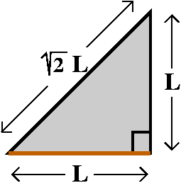 Since in a right triangle,
the hypotenuse is longer than either of the
legs, the only way a right triangle can be isoceles is when the legs
have the same length. And that will occur when both of the acute
angles equal 45o or Π/4 radians. I think that an isoceles
right triangle looks like what is shown to the right. If the base or
bottom side of the triangle (a leg!) has length L, then the height,
another leg, will also have length L, and the hypotenuse will have
length sqrt(2)L. The area of this triangle will be (1/2)L2.
 What can the solid object look like? Here I'll just make an
attempt. If you are new to this stuff, your attempts may not be
terrific the first few times, but they will improve if you practice. I think my version of the
solid looks like what is shown to the right. It has a flat bottom and
a flat side, and the third side is curved, but is made up of lots of
hypotenuses (is that the plural? I also worry about hippopotamuses, or
musi ...). Of course, such solids can't exist in real life, and, for
example, engineers therefore should not worry about them. This is
emphatically NOT CORRECT!!!: all sorts of
machine parts, buildings, and molecules "look" like this. Even if your
first attempt at drawing the solid is not agreeable, I hope that you
will eventually feel you could build one by carving it out of wood or
shaping clay.
Another word ...
I don't think in the previous discussion that I emphasized enough that
the cross-sections were to be perpendicular to the
base. There are lots of ways to slice solids, and then to describe the
solids. I could take a loaf of bread and slice it perpendicular to the
base, the bottom of the loaf. Or I could be more artistic (?) and
slice it in some way that was angled to the base ("obliquely"). Below
is an attempt to show you what I mean. We are analyzing a solid which
is similar to the left-hand loaf of bread, where the slices are
perpendicular to the base.
|
 How to compute the volume
We could get the total amount of bread by adding up the bread in all
the slices. Similarly, we will get the total volume of our solid by
imagining that it is dissected by numerous appropriate slices. To take
advantage of the description, the slices will be parallel to the
x-axis and perpendicular to the xy-plane. We also will think that the
slices are about dy thick. Each individual slice is almost a nice
solid, dy thick, with sides that are almost equal, having an area of
(1/2)L2 where L is the indicated length in the figure. So
dV, a piece of the volume, will be about (1/2)L2dy. And the
total volume is obtained by adding up the pieces of volume, V=∫dV.
Let's be more precise. We will integrate with respect to y. The limits
of integration will be as in the second computation of volume: y=0 to
y=8. The length labeled L here is exactly what I called Width there,
so L=Width=Right(y)–Left(y)=y1/3–(1/4)y, and we need to
compute ∫y=0y=8(1/2)(y1/3–(1/4)y)2dy.
I requested that students complete the computation of this volume
(without any simplification of the answer). This was the Question
of the Day. What is the QotD?
QotD
I'll try to give a simple computation, usually towards the end of each
lecture, which I'll call the Question of the Day. Students get full
credit for handing in any answer. They may work with other
students, use a calculator, look at their notes or textbooks, but they
must hand in some answer. Yes, this a way to take
attendance. It is also a way for me to see if people understand
what I am doing. This is also a way for students, if they wish, to see
if they can do (correctly!) what the lecturer considers to be a
"simple computation".
Here is the computation, which I hope students will do (I haven't yet
looked at the answers).
We can "pull out" the (1/2) but the
best thing to do to the rest is "expand" it (multiply out). Here we
go:
∫y=0y=8(1/2)(y1/3–(1/4)y)2dy=(1/2)∫y=0y=8y2/3–(2/4)y4/3+(1/[16])y2 dy=(1/2)((3/5)y5/3–(3/[14])y7/3+(1/[48])y3(1/2))|08=([128]/[105]) clearly
No, not clearly!!!. In fact, if you had to do this
on an exam or for homework, please report the answer as
(1/2)((3/5)85/3–(3/[14])87/3+(1/[48])83(1/2)). That's a very very good way to report the answer. I
got the number given because a silicon friend told me.
> int((1/2)*(y^(1/3)–(1/4)*y)^2,y=0..8);
                                                128
                                                ---
                                                105
Maybe you should have silicon friends,
also.
Maintained by
greenfie@math.rutgers.edu and last modified 9/3/2009.
 (1/2)cos(θ) sin(θ)+θ/2+C.
 Back to x-land
The translation back turns out to be interesting and more involved
than similar previous transactions. We know that sec(θ)=x and we
want to know what sine and cosine of θ are in terms of x. One way
some people use is drawing a right triangle with one acute angle equal
to θ, and with sides selected
so that sec(θ) is x. Since
(with
some effort) we know that secant is ADJACENT/HYPOTENUSE, and we can
think that x is x/1, well the triangle must be like what is
pictured. Then Pythagoras allows us to get the oppositite side, as the
square root of the difference of the squares of the hypotenuse and the
adjacent side. From the triangle we can read off
sin(θ)=sqrt(x2–1)/x
and cos(θ)=1/x. Then
(1/2)[θ+sin(θ)cos(θ)]+C becomes
(1/2)[arcsec(x)+sqrt(x2–1)/x2]+C. As I explained
in class, arcsec is a fairly loathsome function (yes, this is a
value judgment about a morally neutral function).


 Geometric solution
 A definite integral


 Level 0: Riemann sums, the definition
 What turns out to be important in this business is,
first, how much work is the computation, and second, what sort of
error estimate is valid. Let me copy what I did in class. I looked at
an interval from 0 to small, so you should think of this as a very
narrow interval (yeah, but the picture ...).
 The next trick, straight lines
 Putting it together
 Ha: use three sample points, and parabolas!
 Simpson's Rule
 Here is problem 48 (must be very
difficult!) from section 6.4.
 Pulling a chain up a cliff
 Hooke's Law
 Pulling a spring
 Emptying a pool
 Although the lovely picture above pleases me (artistically!), a more
reasonable view might be sideways. I will put the origin of a
coordinate system for depth at the bottom of the pool (certainly there
may be one or two other reasonable places to put it). Then I will look
at a typical intermediate slice of the water volume at height x from
the bottom of the pool. The slice will have thickness dx. The reason
to look at this is that all of the water in that slice will need to be
lifted the same distance to the top of the pool. So this method of
organizing the computation allows me to put the distance into one part
of the problem, and then concentrate on the force (the weight of the
slice) in another part of the problem. But now we need to think about
the volume of the slice. It is dx thick, and I hope you can see that
the cross-section of the slice is a rectangle. It goes entirely across
the 10 foot width of the pool, and what varies in the slice is the
length, which I labeled L in the diagram. Similar triangles tell me
that L/x=30/7 so that L=(30/7)x. The volume of a slice is
(10)(30/7)x dx, so that the weight of a slice is
(62.5)(10)(30/7)x dx. This slice needs to be lifted to the top
of the pool (not just the top of the water!) and this distance is
1+(7–x)=8–x (I wrote it this way to emphasize that 7–x is the distance
to the top of the water, and 1 more foot to get to the top of the
pool). So the amount of work needed is (8–x)(62.5)(10)(30/7)x dx. To
get the total work I need to add up the work from the bottom of the
water (x=0) to the top of the water (x=7):
 Here of course we will slice the solid dx. The cross-sectional area is
the area of half of a circle whose diameter is L. Well, the area of a
whole circle with radius Π is Π·r2. Here r is
(1/2)L, so that the cross-sectional area is
(1/2)Π[(1/2)L]2. Repeating: the first 1/2 is because we
have half of the area of a circle, and the second 1/2, inside the
parentheses, is because we are changing diameter into radius. Here the
setup is dx. The limits of integration look back to the first
computation of the area, so that x=0 is the lower limit and x=2 is the
upper limit. L is what I called Height then, so
L=4x–x3. What is the volume of the solid? Here we
go. Notice that the (Π/8) factor comes from Π(1/2)(1/2)2
pulled out of the integral (we can do that with multiplicative
factors!).
 Example
 An example
 Formulas for the volumes of all of these solids can be gotten using
the methods of today's class. I'll just do one, the cone. Really this
is called a right circular cone, "circular" because the slices of
the solid perpendicular to its axis of symmetry are circles, and
"right" because the axis of symmetry is perpendicular to the base. The
textbook formula for the volume of a cone with base radius R and
height H is (Π/3)R2H. We can get this cone by revolving
the area under a line segment going from (0,0) to (H,R) around the x-axis.
The slope of this line is R/H, and its equation is y=(R/H)x.

 The Cauchy distribution
 Do all of the homework!
Work with other students!
Read the textbook!
 We slice the area by lines parallel to the y-axis. I think of the
lines as dx apart. The region is chopped up into things which
are almost rectangles, and the area of each piece is going to
be HEIGHT·dx. We will get a good approximation to the total
area by taking the Sum of the areas of
these almost rectangular pieces. Of course what I mean by "Sum" is a definite integral, because that includes
a limiting process which makes increases the accuracy of the
approximations. So in this setup, we will have ∫LeftRightHeight dx. We add up the
slices from the left to the right of the region. Here we have slices
which are dx thick, and we should try to write everything in terms of
x. Let's see: the Left and Right are easy enough, because the
left-most point of the region occurs when x=0, and the right-most
point of the region occurs when x=2. What about the height of the
rectangularish (that's a word?) slice? Well, the height will be the
difference between the top measurement, that is, the curve which forms
the boundary of the region with larger y values, and the bottom, the
curve which forms the boundary of the region with lower y values. This
is a rather simple region, and it isn't too difficult (I hope!) to see
that Top(x)=4x and Bottom(x)=x3. In more complicated cases,
the curves can cross, and to compute the area we may need to break up
the definite integral so cancellation doesn't occur (if you don't know
what I mean, please reread section 6.1, and learn again that
the definite integral computes the net signed area). Please remember
also that the Height will always be given by Top(x)-Bottom(x): this
formula is valid no matter what the signs of the functions are, as long
as Top(x) is geometrically higher than Bottom(x) (well, of
course, since then Top(x)>Bottom(x)).

 I'm really happy that the two results were the same. It turns out (as
you will see in Math 251) that these dual computations are really
quite interesting. We got 12–8=4 and 8–4=4. Some much more
complicated computations are really similar.
 If you are new to this subject, much information is "encoded" in
the paragraph above. I hope you know the base, the bottom of the
solid. It is a flat region in the plane. The solid itself is above
this region. The important sentence in the paragraph is
 Since in a right triangle,
the hypotenuse is longer than either of the
legs, the only way a right triangle can be isoceles is when the legs
have the same length. And that will occur when both of the acute
angles equal 45o or Π/4 radians. I think that an isoceles
right triangle looks like what is shown to the right. If the base or
bottom side of the triangle (a leg!) has length L, then the height,
another leg, will also have length L, and the hypotenuse will have
length sqrt(2)L. The area of this triangle will be (1/2)L2.
 What can the solid object look like? Here I'll just make an
attempt. If you are new to this stuff, your attempts may not be
terrific the first few times, but they will improve if you
 How to compute the volume