Course diary for Math 135, section F2, summer 2006
Monday, August 7
 I "warmed up" by going back to the model of blood circulation. I
briefly discussed how the model might account for heart valves which
don't close all the way: so the blood might slosh (?) backwards
instead of going out and oxygenating the body. So here's the
additional complication which I brought up (and which, sort of,
can actually happen). So I changed the data points for the third and
fourth minutes.
I "warmed up" by going back to the model of blood circulation. I
briefly discussed how the model might account for heart valves which
don't close all the way: so the blood might slosh (?) backwards
instead of going out and oxygenating the body. So here's the
additional complication which I brought up (and which, sort of,
can actually happen). So I changed the data points for the third and
fourth minutes.
Now the question is how much blood is the heart actually pumping out
through the body? Certainly the first, second, and fifth measurements
indicate that blood is progressing outwards. But the third and fourth
measurements show that the heart is pushing back some fluid, so we
should subtract 10 and 8 from the totals for the other minutes.
If you look at the sum, it seems like we are almost trying to
approximate the area of the blood flow which is above the horizontal
axis minus the area below the horizontal axis.
(30 cc/min)·(1 min)+(26 cc/min)·(1 min)+(-10 cc/min)·(1 min)+(-8 cc/min)·(1 min)+(24 cc/min)·(1 min).
Postponing the future value of an income stream
The future value of an income stream is a quantity which attempts to
give a value for various sums of money paid in over an interval of
time. Although the basic idea is closely related to compound interest,
the deals are slightly complicated. If we have enough time next week,
I will attempt to give some idea of this mathematical
"construction".
Velocity/distance problem
A more traditional calculus problem to consider at this stage is a
velocity distance problem. Let me suppose, as I did in class, that a
point moves along a horizontal straight line. Its motion is positive
when the point is moving right. The velocity is negative when the
point is moving left. Let me also suppose that the velocity is given
by the formula v(t)=5t+7 for t in the interval from 1 to 4. Notice
that the velocity is varying. I do know (or, rather, I do believe!)
that if velocity is constant, then DIST=RATE·TIME: distance
traveled in an interval is equal to the product of rate (the
velocity!) multiplied by the time (that, is the duration or length) of
the time interval).
One estimate of distance
I could assume that the velocity is constant, and take as my
"constant" velocity estimate, say, the velocity at time=4 (the end of
the time interval). So the distance estimate is
(5·4+7)(4-1). Maybe this is an o.k. estimate: I am not
particularly interested in doing the arithmetic. Although as I
mentioned, most real-life computations are approximations or
estimations, improving these numbers is usually desirable. How
could an improvement be done?
An improvement
Maybe if we chop up the interval into two pieces, say time varying
from 1 to 2 and from 2 to 4, then separately estimate the velocity in
these two intervals, then compute the resulting distances, and add
these up. Maybe this estimate is closer to the actual distance
traveled by the point. How shall we do this? In the interval [1,2],
maybe I'll see what the velocity is at, oh, 1.5:
(5·1.5+7). I'll multiply this by 2-1, the duration or length of
the interval, and my estimate for the distance traveled will be
(5·1.5+7)(2-1). Then in the interval from 2 to 4, maybe I'll
sample the velocity at 3. My estimate for the distance traveled during
the time interval [2,4] will then be (5·3+7)(4-2).
My total, revised estimate for the distance the point travels from 1
to 4 will be (5·1.5+7)(2-1)+(5·3+7)(4-2).
An improved improvement?
Well, break up the interval [1,4] into [1,2] and [2,3.5] and
[3.5,4]. Then take sample velocities in each subinterval: maybe at 1.5
seconds for the first interval, then 3 seconds for the second
subinterval, and 3.75 seconds for the third subinterval. The
approximate distance traveled in the first subinterval would be
(5·1.5+7)(2-1),
the
approximate distance traveled in the second subinterval would be
(5·3+7)(3.5-2), and
the
approximate distance traveled in the third subinterval would be
(5·3.75+7)(4-3.5). So the total distance traveled using this
approximation scheme is
(5·1.5+7)(2-1)+(5·3+7)(3.5-2)+(5·3.75+7)(4-3.5).
Pictures?
What I've written, even though I have not computed the results, is
already too many numbers for me to understand. I find pictures
easier. But learning what pictures to draw can be difficult.
A graph of the original function
Here is a graph for the velocity function specified,
The information we were given only tells us that the formula is valid
for the interval from 1 to 4. The grpah is part of a line (a line
segment, officially).
|
|
The first approximation: coarse
The estimate was (5·4+7)(4-1). How can this be seen in the
picture? 4-1 is the length of the whole time interval. The other
factor, (5·4+7), is the velocity function at t=4, which is the
height of the graph at the right endpoint of its domain. There are two
lengths involved, and the product could be imagined to be the
area of a rectangle bounded by these two lengths. And that's what I've
attemped to draw and color.
|
|
The improved approximation
The improvement we made resulted in the number
(5·1.5+7)(2-1)+(5·3+7)(4-2).
The first part of this sum is a product, and it comes from the time
interval [1,2]. We use a velocity at t=1.5. The product could be area
of a rectangle whose width is 2-1 and whose height is 5·1.5+7.
The second term that's added is (5·3+7)(4-2). Here the 4-2 is
the length of the second subinterval, and the height is the velocity
at t=3. The product is then the area of a rectangle as shown.
|
|
The improved improvement
This is a somewhat involved sum:
(5·1.5+7)(2-1)+(5·3+7)(3.5-2)+(5·3.75+7)(4-3.5).
The pieces are not that hard to dissect, though. The interval from 1
to 4 is chopped up into [1,2] and [2,3.5] and [3.5,4]. The second
factors in each of the parts of the sum are the lengths of these
subintervals. The first parts are velocities at some (more or less
randomly chosen!) times in each of these subintervals: t=1.5 and t=3
and t=3.75. Actually these t's happeen to be the middle of each
subinterval. The velocities are the heights of three rectangles, and
the total sum is the total area of three rectangles.
|
|
The calculus vocabulary again (maybe for the last time!)
By now you should see that, whatever the heck we are doing, it is
very complicated and hard to compute. So let me retreat, the
way an academic is supposed to, and define everything in sight. Then
I'll return with more examples.
Suppose we a given a function f(x) defined on a
closed interval [a,b].
- A partition of [a,b] is a collection of points
(including the endpoints a and b) which divide the interval up into a
"bunch" of subintervals. If we want to have n subintervals (here n is
a positive integer) then (think about this, please) we need n+1
points. If a and b are two of the partition points, we need n-1 of
them on the inside. Her is the mostly traditional algebraic
labeling:
a=x0< x1<
x2<x3< ...xn-3<
xn-2< xn<=b.
The subintervals are then [x0,x1] and
[x1,x2] and [x2,x3] and ...
and [xn-2,xn-1] and
[xn-1,xn]. The ith subinterval is
[xi-1,xi].
Each subinterval has a length which is the right-hand endpoint
minus the lefthadn endpoint. The length of
[x0,x1] is
x1-x0, for example. The length of the
ith subinterval,
[xi-1,xi], is xi-xi-1.
Unfortunately for the novice there is also some traditional rather
irritating notation which is used for these
lengths. x1-x0 is frequently abbreviated (and
not only in math classes, darn it!) as  x1. The length of the th subinterval,
[xi-1,xi], is xi-xi-1 is
also called xi.
x1. The length of the th subinterval,
[xi-1,xi], is xi-xi-1 is
also called xi.
- One sample point is selected inside each subinterval. The
first subinterval, [x0,x1], therefore has one
specially designated point, which I'll call
x1*. This seems fairly standard notation in many
calculus books but maybe not in too many areas outside of math.
Right now I don't know too much about x1* except that a=x0≤x1*
and x1*≤x1. These inequalities just tell
me that the point is indeed inside the first subinterval.
The ith subinterval, [xi-1,xi], has
a designated sample point inside it: xi*.
- The Riemann sum associated with the function f(x), the
closed interval [a,b], and the choices of partition and sample points,
is the following:
f(x1*)(x1-x0)+f(x2*)(x2-x1)+f(x3*)(x3-x2)+...+f(xn-1*)(xn-1-xn-2)+f(xn*)(xn-xn-1).
 A picture
Riemann sums are very complicated to me. I've tried to sketch a
picture to the right. The picture is suppose to represent a Riemann
sum. There are the first two rectangle sand the last two
rectangles. You might observe, I hope, that each piece of the sum
represents a height (a value of f(x) at a sample point) multiplied by
the appropriate length of a subinterval. So the pieces of the Riemann
sum are areas of these rectangles.
The idea is that these sums form a "fomral" way of writing the
approximating ideas which I have shown you for blood flow and distance
and area and ... many other things. I don't believe it is likely that
you will compute many slopes in your lives and careers after Math 135,
but I really do think you will compute (acknowledged or not!)
many Riemann sums!
Riemann sum: example #1
The function: f(x)=x2; the interval: [1,4]; partition: 1,
1.5, 2, 3, 3.5, 4 (so five subintervals); sample points: 1.25, 1.8, 2,
3.5, 3.5.
The sum is:
(1.25)2(1.5-1)+(1.8)2(2-1.5)+(2)2(3-2)+(3.5)2(3.5-3)+(3.5)2(4-3.5).
Comments Yes, notice that sample points can "repeat" but just
once (a right-hand endpoint for one subinterval can be used and then
reused as a left-hand endpoint for the next subinterval). I remarked
that although I've seen using sort of "random" sample points, in fact,
much of the time there is considerable care taken in choosing
them. Frequent choices are midpoints of subintervals or left- or
right-hand endpoints. In the "real world" the number and spacing of
sample points might be complicated and expensive: drilling oilwells or
taking surveys of populations or ...
Riemann sum: example #2
The function: f(x)=1/x; the interval: [2,6]; the partition: 2, 3, 5, 5.5,
6 (so four subintervals); the sample points: the midpoints of each
subinterval.
In [2,3], the sample point will be 2.5 (that's {2+3}/2). In [3,5], the
sample point will be 4. In [5,5.5], the sample point will be 5.25. In
[5.5,6], the sample point will be 5.75.
The sum is:
(1/2.5)(3-2)+(1/4)(5-3)+(1/5.25)(5.5-5)+(1/5.75)(6-5.5).
And I won't do the arithmetic unless I must!
Regular partitions
Also the partitions are usually not chosen so randomly, either. A
regular partition has subintervals with equal lengths. Let's try an
example.
Riemann sum: example #3
The function: f(x)=x3; the interval: [0,6]; the partition:
a regular partition with 100 intervals; the sample points are the
right-hand endpoints of each subinterval.
Since we're dividing the interval [0,6] into 100 equal pieces, the
length of each piece is 6/100 which is .06.
I asked students to write the first three and last two pieces of the
Riemann sum. Here they are:
(.06)3(.06)+(.12)3(.06)+(.18)3(.06)+ ...(5.88)3(.06)+(6.)3(.06).
O.k., o.k., some numbers
The value of that crazy sum is
330.5124. It turns out there is a really, really slick way to compute
what this approximates (huh?) and the "true value" is 324. I will show
you how to do this within 48 hours!
Notation that is useful but does repel novices!
 The Riemann sum above can be written in words using some phrasing
similar to the following:
The Riemann sum above can be written in words using some phrasing
similar to the following:
The Riemann sum is the sum as the integer i goes from 1 to 100 of the
cube of the number .06 multiplied by the integer i, which is then
multiplied by .06 .
To the right is notation for this which is about 350 years old. The
word "sum" is abbreviated by the initial letter (in Latin!) of sum.
That is a Greek capital sigma. You should see this so that its
appearance will not frighten you at some other time in your
life (if it is being used by a salesperson to amaze and
awe you and convince you to buy unsuitable insurance or
something.
 To the right is the horrifying algebraic formulation of the "general"
Riemann sum. There's the function, f(x), evaluated at the sample
point, and multiplied by the widths of the subinterval (don't neglect
the 's, also!). The "lower limit"
on the capital sigma says "Start adding these things up when i is 1"
and the "upper limit", n, says keep adding them until you get to the
nth term. I will try to avoid using this notation, but you
are likely to see it sometime, so you should please not shriek when
you see it.
To the right is the horrifying algebraic formulation of the "general"
Riemann sum. There's the function, f(x), evaluated at the sample
point, and multiplied by the widths of the subinterval (don't neglect
the 's, also!). The "lower limit"
on the capital sigma says "Start adding these things up when i is 1"
and the "upper limit", n, says keep adding them until you get to the
nth term. I will try to avoid using this notation, but you
are likely to see it sometime, so you should please not shriek when
you see it.
Wednesday, August 2
I began by stating that the course will conclude with
- The definition of one more complicated concept
- A wonderful and unexpected and powerful result relating this new
concept to the stuff we've been doing.
I will give two motivational examples for the concept. One will
involve blood flow from biology (medicine) and one will discuss
future value of a income stream (business or economics). Here
is the first example.
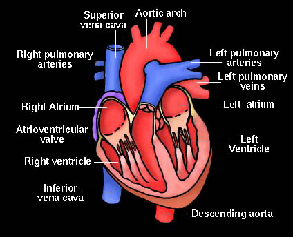
Blood flow
Suppose we now consider the following interesting physiological
problem. A diagram of the human heart is shown. Blood flow through
various "pipes" in the system is known to be an important indicator
of health. How can we measure the blood flow through the aorta, the
major artery emerging from the heart?
| 
|
The Aztec solution
One method might be to take a knife, preferably an obsidian
knife, and rapidly cut through the chest wall, sever the aorta, and
cause the blood that would flow through it to fill up a bucket. In
about five minutes we'd probably have a good idea of how much blood
flows through the aorta. There are several criticisms possible of this
"protocol". One namby-pamby criticism (my online dictionary declares
that "namby-pamby" means "insipidly pretty or sentimental") might be
that, well, maybe the person involved might not be good for much
afterwards. Another criticism could be that this would not show the
actual pumping capacity of the aorta, because maybe within a minute or
two some ... difficulties would occur. In some sense, this Aztec
protocol is the ultimate in what might be called destructive
testing.
|

|
Another solution: cardiac catheterization
The American Heart Association and the NIH (National Institutes of
Health) both have lots of information about this. So:
-
The AHA begins:
This is a procedure done on the heart. In it, a doctor inserts a thin
plastic tube (catheter) (KATH'eh-ter) into an artery or vein in the
arm or leg. From there it can be advanced into the chambers of the
heart or into the coronary arteries.
- Or from
the NIH:
Cardiac catheterization is used to study the various functions of the
heart or to obtain diagnostic information about the heart or its
vessels. A small incision is made in an artery or vein in the arm,
neck, or groin. The catheter is threaded through the artery or vein
into the heart. X-ray images called fluoroscopy are used to guide the
insertion.
Very much simplified ...
Imagine a thin plastic coated wire inserted into your circulatory
system and threaded up into the aorta. At the end of the wire is a
sort of microscopic windmill: a bunch of little fans which spin as the
blood flows. As they spin, they move a magnet around a bunch of
wire. Since magnetism+movement+wires=current ( a wonderful
fact!), electrical current is created and passed back through the wire
into a measuring device. This is certainly very much simplified. Now I
will further simplify and imagine some numbers. This is not reality,
but a math course! The following numbers are invented, and the whole
purpose of this "exercise" is to get you to think about what's going
on.
At the
end of |
Minute #1 |
Minute #2 |
Minute #3 |
Minute #4 |
Minute #5 |
|---|
blood flow
rate is |
30 cc/min |
26 cc/min |
28 cc/min |
36 cc/min |
24 cc/min |
|---|
As I mentioned in class, maybe the reason for the jump at the fourth
minute is because a calc instructor walked into the room and murmured,
"Chain Rule!" How can we use this information to get an
approximation to the "real" blood flow? You might make the assumption
that, hey, maybe the flow rate doesn't change too much in a minute,
and maybe we can approximate the total blood flow by assuming the flow
rate is constant during that minute. So then during the first minute,
when the only measurement we have is 30 cc/min (cubic cows? no, cubic
centimeters), we could conclude that during the first minute the total
flow is (30 cc/min)·(1 min).
The units cooperate --
that is, the minutes cancel, and we see that 30 cc's (maybe) flowed
through
the aorta in the first minute. During the second minute, we have the
measuement (at the end of the second minute) of 26 cc/min. Therefore,
same (perhaps and probably not totally correct) assumptions show that
blood flow in the second minute is (26 cc/min)·(1 min).
Etc.. The answer that we can get from the
information supplied seems to be:
(30 cc/min)·(1 min)+(26 cc/min)·(1 min)+(28 cc/min)·(1 min)+(36 cc/min)·(1 min)+(24 cc/min)·(1 min).
I am not interested in these particular numbers, but I am very interested
in the ideas they represent.
A better approximation
We might want a better approximation to the blood flow. I
do not think it is realistic to assume that blood flow is steady, and
jumps only at the minute marks. To improve our information, with just as
much investmant in the (imagined!) equipment, we could (imagine!)
examining and recording flow rates every 30 seconds during the 5
minutes. We might get some data like this:
At the
end of |
30 seconds |
Minute #1 |
1 minute
30 seconds |
Minute #2 |
2 minutes
30 seconds |
Minute #3 |
3 minutes
30 seconds |
Minute #4 |
4 minutes
30 seconds |
Minute #5 |
|---|
blood flow
rate is |
26 cc/min |
30 cc/min |
27 cc/min |
26 cc/min |
29 cc/min |
28 cc/min |
31 cc/min |
36 cc/min |
38 cc/min |
24 cc/min |
|---|
Again, there are lots of numbers. So what? How can we use these
numbers? To begin, how could we use the measurement at 30 seconds? We
could assume the flow rate of 29 cc/min is constant during that
initial 30 seconds. Then the blood flow would be ... well, should I
write 29·30? No: we shouldn't get confused about units. The
time is in minutes, so 30 seconds is (1/2) minute. In fact, the new
information allows us to write the following (probably better)
approximation to the blood flow: (I am omitting the units here because
I am a math geek.)
(26)·(1/2)+(30)·(1/2)+(27)·(1/2)+(26)·(1/2)+(29)·(1/2)+(28)·(1/2)+(31)·(1/2)+(36)·(1/2)+(38)·(1/2)+(24)·(1/2).
What is going on? The number of terms to add is increasing, but if you
look very very carefully you will see that each term individually is
getting smaller. In fact, these changes nearly balance: more
terms/smaller terms. The totals are different, but not very
different. The new total is "better", a refinement of the old sum. The
approach here is computational and numerical, and for me obscures
what's going on. A collection of pictures actually provides far more
information for me here.
Approximating what, "exactly"?
Well, we began by using only the information at five different times,
at the end of each minute. If we were to plot points on a graph of
blood flow, we would see the picture to the right. The first sum we
wrote is exactly the total area under the five boxes shown,
with "area" interpreted as the amount of blood.
|
|
|
When we put in the data points at 30 second intervals, we can see
pictorically exactly what that second crazy sum represents: it is the
total area in the boxes of width (1/2) minute, with "area" interpreted
as the amount of blood.
|
|
|
Now what do the "Aztecs" get as their information? We could
imagine a flow rate function which sort of threads its way
through the data points supplied. The Aztecs, with the ridiculous
bucket holding exactly the blood going through the aorta, would have
an amount of blood which is exactly the area under the blood rate flow
graph. You can see that we have these rectangular
approximations to the area which we hope get better as the rectangles
get thinner and the number of samples of the flow rate increases.
|
|
The idea is that we can estimate the blood flow by doing a
collection of flow rate measurements, multiplying by the length of the
appropriate time intervals. This sum approximates the true amount of
blood going through the aorta. But if we wanted a better estimate, we
should then increase the number of observations, followed by, in each case,
multiplying by the length of the appropriate time interval and then
summing. If we took many measurements, and if we distributed
the measurements evenly or uniformly along the time interval then we
would hope the estimate we'd get would be close to the true amount of
blood pumped. Notice, though, that even if we increasing the number of
measurements to, say, 10,000, if we clustered the measurements (only 1
in the first 4 minutes, and then 9,999 in the last minute) we should
not really expect the approximation to be good. A good approximation
will be obtained if the number of measurements is large and if the
measurements are well distributed in time.
Tuesday, August 1
Let's see: with the able efforts of several students, and, in one
case, with the incredibly bad typing of the instructor
(explained below!), we worked on various problems involving implicit
differentiation and linear approximation.
Problem 1
This problem seemed to be correctly stated and was
done well by students. It illustrated what's good and what's bad about
explicit and implicit definitions of functions. Problem 2 was supposed
to show that some calculus can still be done with an implicitly
defined function which could not easily (or at all, based on methods I
know!) be turned into an explicit formula.
Problem 3
 Here we needed to get a formula for
dy/dx from the defining equation of the ellipse,
x2+xy+y2=5. We did this.
Here we needed to get a formula for
dy/dx from the defining equation of the ellipse,
x2+xy+y2=5. We did this.
d/dx the equation and get 2x+1·y+x·(dy/dx)+2y(dy/dx)=0
gives
(2x+y)+(x+2y)(dy/dx)=0 so that
dy      2x+y
-- = - ------
dx      x+2y
Then we "realized" the
sides of the bounding box for the ellipse were parts of
vertical and horizontal lines which were tangent to the ellipse. Since
horizontal tangents are characterized by dy/dx=0, we were able to get
the TOP=0 together with the defining equation and deduce what
the points were:
Since 2x+y=0, y=-2x and then
x2+xy+y2=5 becomes
x2+x(-2x)+(-2x)2=5 and (1-2+4)x2=5 so
x=+/-sqrt{5/3}. The y-coordinates are gotten from y=-2x. There are two
points with horizontal tangents, and they correspond to the + sign for
the bottom and the - sign for the top, because the bottom point of
tangency (for the horizontal line) is further to the right than the
top point.
A bright idea (really!) was to remark that vertical
ines are lines which have no slope. Therefore we need to
combine some condition on the dy/dx formula guaranteeing there is no
slope together with the defining equation. This we decided would be
when BOTTOM=0, where BOTTOM was the bottom,
denominator, of the fractional formula which gave dy/dx. And actually
this worked, because when we try to find simulatneous solutions of
BOTTOM=0 and the defining equation, we got the two points on
the ellipse which correspond to the points where tangent lines are
vertical. The actual numbers involve sqrt(5/3). To the right is a
graph of the ellipse together with its bounding box. The light green horizontal lines have the
equations y=+2sqrt(5/3) and y=-2sqrt(5/3). The blue vertical lines have the equations
x=2sqrt(5/3) and x=-2sqrt(5/3).
Problem 2 as it should have been!
Well, the instructor typed wrong. The formula he should have typed
is
ex-xy+3cos(x2-y)=4
and let me analyze this formula. The change is x-xy in the
exponential rather than y-xy. First, the point (1,1) does satisfy
this formula, since
e1-(1·1)+3cos(12-1)=e0+3cos(0)=1+3=4.
Good start, I guess. Now how about a line tangent to the curve defined
by this equation at the point (1,1)? For this I will differentiate the
defining equation with respect to x, assuming that y is
implicitly defined as a function of x by the equation. So the
Chain Rule etc. gives the following result after "d/dx":
ex-xy(1-y-xy´)-3sin(x2-y)(2x-y´)=0
I am using y´ instead of dy/dx here. Now if we "plug in" 1 for x
and 1 for y we get:
e1-(1·1)(1-1-y´)-3sin(12-1)(2·1-y´)=0
Since e0=1 and sin(0)=0 this becomes just y´=0: the
derivative is 0. The tangent line is horizontal. A picture of the
curve and a segment of the horizontal tangent line through (1,1) is
shown to the right. The second picture is a close-up of the point of
tangency, with a portion of the curve and the tangent line.
| 
|
Problem 2 as it was
In the original problem 2 we started with:
ey-xy+3cos(x2-y)=4
and again (1,1) satisfies this equation. So d/dx the equation, and the
result is:
ey-xy(y´-y-xy´)-3sin(x2-y)(2x-y´)=4
Let me "solve" for y´ here. Here I distribute:
ey-xyy´-ey-xyy-xey-xyy´-6xsin(x2-y)+3sin(x2-y)y´=0
and now collect terms:
[ey-xy-xy+3sin(x2-y)]y´+[-ey-xyy-6xsin(x2-y)]=0
and finally solve for y´ (the minus signs cancel when we throw
stuff to the "other side"):
y´=[ey-xyy+6xsin(x2-y)]/[ey-xy-xy+3sin(x2-y)]
If we "plug in" x=1 and y=1 in this formula we'll get 1/0: the slope
does not exist -- just as in problem 3, the tangent line is a vertical
line. Sigh.
A picture of the
curve and a segment of the vertical tangent line through (1,1) is
shown to the right. And, again, the second picture is a close-up of the point of
tangency, with a portion of the curve and the tangent line.
| 
|
Problem 4
Parts a) and b) and c) are straightforward if the powers of 10 can be
kept organized. For part d), the second derivative computation needs
to be done carefully, and, as we saw, the sign of f´´(1) is
negative so the curve is concave down and the true values are
less than the linear approximations. (This all didn't come out well in
class, but then ... perfection is rarely attained, but should always
be our target.)
Problem 5
The surface area/volume relationship is the most interesting: increase
volume a bit, and the linear approximation actually overstates the
surface area, so there is less surface area than might be
expected by carelessly using linear extrapolation. High volume people
might have less surface area than one might expect by studying low
volume people.
Problem 6
From www.investorwords.com:
widget
Definition: A hypothetical product used to illustrate a business concept.
From whatis.techtarget.com:
widget
1) In general, widget (pronounced WIH-jit) is a term used to refer to
any discrete object, usually of some mechanical nature and relatively
small size, when it doesn't have a name, when you can't remember the
name, or when you're talking about a class of certain unknown objects
in general. (According to Eric Raymond, "legend has it that the
original widgets were holders for buggy whips," but this was possibly
written tongue-in-cheek.)
The Oxford English Dictionary (a mighty authority!)
declares that widget means
An indefinite name for a gadget or mechanical contrivance, esp. a
small manufactured item.
and that the word was first printed in 1931.
Yes, the trip should be taken, and cutting the ad budget probably
would result in a net savings.
Problem 7
We never did discuss problem 7.
I wrote the following to help you realize what I think the second exam
is about:
- Differentiation methods
- Chain rule (on the formula sheet)
- Implicit differentiation
- Related rates
- Tangent line/differential
- Formula (on the formula sheet)
- Error {up|down} (from concavity of the function)
- MVT
- The statement: how it relates f´(x) and f(x).
- If f´(x)>0 then f(x) is increasing.
- If f´(x)<0 then f(x) is decreasing.
- Vocabulary
- {In|de}creasing
- Concave {up|down}
- Relative {max|min}
- Critical {number|point}
- Inflection point
- Absolute {max|min}
- Curve sketching
- Going from formula to picture
- Draw pictures given function properties
- Using the vocabulary (above) to describe pictures
- Asymptotes
- Horizontal: relies on limits as x-->+/- infinity;
possible use of l'Hop.
- Vertical: relies on limiting behavior near endpoints
or holes in the domain.
- Max/min: optimization
- Check critical numbers
- On an interval with endpoints: test endpoints also
- On open interval, what happens towards the edge
- Why a max or a min?
The zeroth derivative test: does the function have
enough information to make conclusions about max/min?
- Why a max or a min?
The first derivative test: use sign of f´(x).
- Why a max or a min?
The second derivative test: use sign of f´´(x).
100oF or 37o is hot anywhere.
Monday, July 31
We discussed the assigned related rates problems. Some students put
some of these problems on the board. It is frequently important to
assign variables to the problems, draw pictures, use geometry or other
aspects of these problems to write equations relating the variables,
and (most important) write clearly what is given and what is
requested. The problems we looked at involved ladders and right
triangles and led to a right triangle (similar to the distance problem
involving Herman and Nancy and Cedar City last time), spheres (a
helium balloon and a hot-air balloon), and circles (the changing
ripples after a rock is dropped into a pond). It is usually good to
see if the signs (increasing/decreasing) of the answers agree with
"intuition".
I "invented" a problem which started with
a rather ludicrous basic assumption (the numbers are a bit different
from what I used in class):

Suppose the sides of a rectangle vary with time. At a certain time,
the length of the rectangle is 20 inches and is shrinking by 1 inch
per second. At that time, the width of the rectangle is 5 inches and
is increasing by 1/3 inch per second.
Question 1
What is the rate of change of the rectangle's area at "that time"? Is
the area increasing or decreasing then?
We know that
A=LW, so A´=L´·W+L·W´. At "that time",
A´=(-1)(5)+(20)(1/3)=-5+(20/3)=+5/3. The area is
increasing at "that time".
Question 2
What is the rate of change of a diagonal's length of the rectangle at
"that time"? Is the diagonal's length increasing or decreasing then?
I first compute D at "that time": Since
D2=L2+W2,
D2=202+52=425, so D=sqrt(425). But we
can also use the equation D2=L2+W2 to
get information about rates of change. We d/dt this equation and see
that 2D·D´=2L·L´+2W·W´. Therefore
2sqrt(425)(dD/dt)=2·20(-1)+2·5(1/3)=-110/3. Therefore
dD/dt=-110/[6sqrt(125)]. The diagonal's length is decreasing at
"that time".
I changed the numbers so I could get one of the quantities decreasing
and the other increasing. That such different behavior could happen is
perhaps not so obvious.
For us the related rates especially seem like "toy" problems to
me. The problems which occur in reality that resemble these involve
more complicated linking equations and the data is also not simple.
Linear approximations/tangent line
approximations/marginal analysis, elasticity ...
I copy the following from the diary
entry of Wednesday, July 5:
If a function is differentiable, then we know that
limh-->0[f(x+h)-f(x)]/h=f´(x). This statement may no
longer be precisely correct if "limh-->0" is omitted. ...
... what we have is
[f(x+h)-f(x)]/h=f´(x)+Err(h)
where Err(h) is some sort of error function which -->0 as h-->0.
We could then multiply the equation by h and get
f(x+h)-f(x)=f´(x)h+Err(h)h
and add f(x) to both sides and
get
f(x+h)=f(x)+f´(x)h+Err(h)h
Certainly you should see, I hope, I hope, again something which was
mentioned repeatedly last week. If we kick or perturb the input to
f(x) and if we know that f(x) is differentiable, then the kicked or
perturbed output will be the old output plus a term directly
proportional to the disturbance (this is what's called in economics
the marginal response) plus, well, Err(h)h. Since I think of h as
small and Err(h) is also small, well, the product is even smaller
still. That's the important idea. |
The geometric idea is shown in the picture to the right. Well, it is a
complicated picture. The tangent line has slope f´(x). The tiny
right triangle shows OPP and ADJ: these are related
by the tangent of  , which is
the slope of the line. So OPP/ADJ=f´(x) and
since ADJ is h,
OPP=f´(x)ADJ=f´(x)h. Therefore the length
f(x+h) is written as a sum of f(x) and =f´(x)h and another piece, very tiny (at least in the picture!),
shown in red with a ? near it. The
diagram is drawn to be persuasive, of course (but wait for the example
below!):
, which is
the slope of the line. So OPP/ADJ=f´(x) and
since ADJ is h,
OPP=f´(x)ADJ=f´(x)h. Therefore the length
f(x+h) is written as a sum of f(x) and =f´(x)h and another piece, very tiny (at least in the picture!),
shown in red with a ? near it. The
diagram is drawn to be persuasive, of course (but wait for the example
below!):
f(x+h)=f(x)+f´(x)h+Err(h)h
In economics, the multiplier of h might be called the elasticity or
the marginal "something" or the ... and the replacement of f(x+h) by
f(x)+f´(x)h is justified whenever h is relatively small.
Now some numbers
First
Let me try almost the simplest non-linear function:
f(x)=x2, so f´(x)=2x. We certainly know that
f(3)=9 and f´(3)=6. What about f(3.04)?
The tangent line approximation will the actual value with
f(3)+f´(3)(.04) if we take h to be .04, and so the approximate
value is 9+6(.04)=9.24. The actual value is 9.2416.
Second
Well, we can also do 2.92, with the same f(x) and same x=3, but with
h=-.08 (h's can be negative as well as positive). Then the linear
approximation is f(3)+f´(3)(-.09)=9+6(-.08)=9.52. The actual
value is 8.5264.
Third
Let's compute f(10) using the same f(x) and the same x=3, but with
h=7. Then f(3)+f´(3)(7)=9+6(7)=51. Well, f(10)=102=100
and 100 does not see very close to 51. I guess that h=7 is not
"relatively small".
I don't think I can give you good and always suitable advice. The uses
of the linear approximation idea are everywhere. Almost surely a
doctor has used it on you: hey, this medication has a standard
dose of 12 milligrams, but this person is not average in their
weight/activityy/metabolism, so we should {in|de}crease the dosage by
the following amount per ... and those increases are mostly done by
linear approximations to various mathematical models. They should not
be extrapolated too much: I'll bet there are medications whose dose
for a 250 pound person shouldn't be double the dose for a 125 pound
person.
There is one more neat thing that can be done "by hand" to check on
the suitability of linear approximation. Let me illustrate this with
an example. Suppose f(x)=7e3x-2x2-1. I know that
f(1)=7e0=7 (I chose this function so that f(1) will be easy
to compute). Then I know (Chain Rule!) that
f´(x)=7e3x-2x2-1(3-4x), and I evaluate at
x=1: f´(x)=7e0(3-4)=-7. An approximate value of
f(1.03) using the tangent line approximation (with x=1 and h=.03) is
f(1)+f´(1)·(.03) and this is 7+(-7)(.03)=6.79. O.k. so far
-- more or less like we've already done. But now a different question:
 [Over|Under]?
If 6.79 an overestimation or an underestimation of the "true value" of
f(1.03)? The "nuance" of this question may not be totally clear. The
picture is an effort to show what's going on. We know that y=f(x)
(this f(x)!) goes through the point (1,7) and that its tangent line at
that point has slope -7. The number 6.79 results from assuming that
the graph of y=f(x) near x=3 is close to the tangent line drawn, and
that 1.03 is close enough to 1 so that the value on the tangent line
is close to the "real" value on the curve. A piece of the curve itself
near x=1 could possibly look like the green curve below the tangent
line or like the red curve above the tangent line. Can we decide which
without extensive work or use of resources (that is, a computational
device?). What determines the local relationship between the curve and
its tangent line is the second derivative at that point, which shows
if the curve bends up (the red curve, when the second derivative is
positive) or if the curve bends down (the green curve, when the second
derivative is negative). That is, the {above|below} and {over|under}
here is determined by concavity.
The concavity of the graph near x=1 can be seen by computing
f´´(x) and evaluating the result at x=1. Since
f´(x)=7e3x-2x2-1(3-4x) we compute the
second derivative carefully. We need to use both the product
rule and the chain rule. Here's the result:
 f´´(x)=7e3x-2x2-1(3-4x)2+7e3x-2x2-1(-4)
which makes f´´(1)=7e0(-1)2+7e0(-4)=7-28=-21.
The graph is concave down (the green choice) and the "true value" is
below the linear approximation. By the way, the "true value" can of
course be computed, and it is 6.7809, which is less than 6.79, our
tangent line approximation. The graph to the right is what the darn
thing really, really looks like, and below is a stretched version
(2:25 in horizontal:vertical ratio!), making the graph perhaps easier
for human beings to appreciate.
I don't believe the [Over|Under]? question is another
mathematical "hoop" for you to jump through, and learn in the most
superficial fashion. Please consider again the data we looked at before formally
defining and systematically investigating concavity. I hope that the
difference between positive and negative second derivatives,
especially when considering numbers involved in public policy, makes
the occasional importance of what we're considering clear.
Thursday, July 27
Students kindly put a few more textbook problems on the board. We
discussed constraints and objective functions, how to determine
relevant domains, and why the designated answers were actually the
correct extreme values. We used the techniques mentioned last time to
answer the why's about why should "this" be a maximum or minimum value
(the Zeroth and First and Second Derivative Tests).
A darling problem
My darling ... is in trouble. MD (my darling) is struggling in the
ocean, a half-mile offshore, 4 miles down from me along a straight
beach. Suppose that I can run (hah, if only I could!) at 10 mph, and
swim at 4 mph (even more of a joke). What is the best strategy for me
to get to MD in the least amount of time?
This is a complicated problem, and we need to discuss it. There are a
variety of strategies for "Me" to get to MD. The strategies can be
analyzed by assuming that they all consist of running along the beach
for a distance of x miles in a straight line, followed by swimming
along a straight line to the darling. One extreme "pure" strategy is
gotten by taking x=0: the tortoise strategy. This is shown in the
yellow line straight from me to MD. I might want to follow that
strategy if I were a huge turtle. My running speed would then be
rather low, but my swimming speed would be relatively high. I hope you
can see that the "all swimming" strategy then would be a winner, the
least time path. On the other hand, if I were, uhhhh ...., something
which could run very fast but swim really slowly (a cheetah: cheetahs
can swim) the best strategy would likely be to run as much as
possible and swim as little as possible. This would correspond to x=4,
shown in red on the picture. So if I could run at 100 mph and swim
very slowly, the cheetah strategy would clearly be the best.
Analysis of a general mixed strategy, the dashed green path
If I run x miles, then (at 10 miles per hour, with
distance=rate·time) the running time would be x/10. How long a
distance will I need to swim? Well, the tilted part of the dashed
green path is the hypotenuse of a right triangle. The remaining beach
distance is one leg of the right triangle, and is 4-x miles, while the
other leg is 1/2, the miles the darling is offshore. Then Pythagoras
gives the swimming distance as
sqrt{(x-4)2+(1/2)2}, so that (rate/time/distance
again) the swimming time is
sqrt{(x-4)2+(1/2)2}/4. Hey, this is some
function. (Dist=rate·time, so time=dist/rate.)
Darling time
So we need to find the minimum of
f(x)=(x/10)+sqrt{(x-4)2+(1/2)2}/4 with domain
0≤x≤4.
As I remarked in class, in 1906 we would need to stay in the Church of
Math 135 (this was not meant to be offensive to any church or any
religion or any person ... it is just an extended metaphor). A picture
of the church, with its extremely elaborate nondenominational stained
glass windows, is
shown here. What do I mean by "stay in the Church"? So here I tell you
to solve the problem in the following way:
Differentiate
f(x); do the algebra necessary to find the critical number(s) (maybe
your intuition tells you there is exactly one critical
number!); compare the value (the time needed) at the critical number
to the times at the end (the pure tortoise and pure cheetah strategies),
and report back with the least time answer.
 The current
year is 2006. I would certainly begin by graphing f(x) in the interval
[0,4]. I'd see that there is actually an interior minimum (inside the
interval, fairly close to 4). I did not anticipate the tiny
"hook" when I wrote the numbers 10 and 4 in the statement of the
problem. And you can even numerically approximate
this answer: it is about 3.78 miles and the minimum time
(corresponding to this choice of strategy) is abpit .51 hours. You can
get this with not very much work. If you face problems such as these
in your courses or careers, use the resources that progress has given
us, please: you may leave the orthodox Church of Math 135.
The current
year is 2006. I would certainly begin by graphing f(x) in the interval
[0,4]. I'd see that there is actually an interior minimum (inside the
interval, fairly close to 4). I did not anticipate the tiny
"hook" when I wrote the numbers 10 and 4 in the statement of the
problem. And you can even numerically approximate
this answer: it is about 3.78 miles and the minimum time
(corresponding to this choice of strategy) is abpit .51 hours. You can
get this with not very much work. If you face problems such as these
in your courses or careers, use the resources that progress has given
us, please: you may leave the orthodox Church of Math 135.
Actually, the most amazing thing is that you really, really can stay
"inside" the Church and have the work done for you. For example, the
exact answer to the previous problem is x=4-(21)-1/2. There
are machines which can do the symbolic manipulation, provided that
you know enough to guide the machines. One program which can do
this is Maple
, available on most Rutgers
systems (including the main student system, eden. There are
other programs which can do this, as well as some hand-held devices,
such as the TI-92. Just to show you what the heck can be done, what follows is
part of a Maple dialog (I made many typing errors, and this
is cleaned up quite a bit). My input is typed after each >
and then Maple responds, displaying an answer to the
input.
Here is where I defined f for Maple.
 f := 1/10*x+1/4*sqrt((x-4)^2+(1/2)^2);
                                                    (1/2)
                         1      1 /   2            \
                    f := -- x + - \4 x  - 32 x + 65/
                         10     8
I found the derivative of f.
> g := diff(f, x);
                         1             8 x - 32
                    g := -- + --------------------------
                         10                        (1/2)
                                 /   2            \
                              16 \4 x  - 32 x + 65/
I asked that the derivative be simplified.
In this case, the program combined things into one fraction. It also
decided that the whole mess was too long to type on one line, so it
"abbreviated" with the %1 equation.
> h := simplify(g);
                                  %1 + 5 x - 20
                             h := -------------
                                      10 %1
                                                (1/2)
                              /   2            \
                        %1 := \4 x  - 32 x + 65/
I found the top of the derivative.
> k := op(2, h);
                                          (1/2)
                        /   2            \
                   k := \4 x  - 32 x + 65/      + 5 x - 20
I isolated the square root by canceling
the 5x+20, and then squared.
> m := (k-5*x+20)^2;
                                    2
                            m := 4 x  - 32 x + 65
Here I squared the term I took away.
> n := (5*x-20)^2;
                                             2
                              n := (5 x - 20)
Here it is "expanded". I am solving the
algebraic equation sqrt(A)+B=0 by writing sqrt(A)=-B and then
A=B2 and then A-B2=0. I hope this helps. The A
term is above. The B2 term is below.
> p := expand(n);
                                   2
                          p := 25 x  - 200 x + 400
Now A-B2. I am collecting terms
on one side of the equation. It is a quadratic equation.
> q := m-p;
                                    2
                          q := -21 x  + 168 x - 335
Here are the roots.
> solve(q);
                           1    (1/2)      1    (1/2)
                       4 - -- 21     , 4 + -- 21
                           21              21
And here are the approximate numerical values.
> evalf(solve(q));
                          3.781782110, 4.218217890
Just so you can see it, the darn program can do all of the work in one line:
> solve(diff(f, x));
                                   1    (1/2)
                               4 - -- 21
                                   21
or if you want an approximate answer, here is a one-line command:
> evalf(solve(diff(f, x)));
                                 3.781782110
I don't think that Maple can read a natural language problem and solve
it. And, although the program is very powerful, unless you sort of
know what "shape" the answers should be, you can really make lots of
mistakes very fast. Here it resembles the simplest kind of mechanical
calculator which could possibly respond to the request 23+67 with the
answer 203,407: I think people should know enough about arithmetic to
realize that the answer is incorrect. Programs with more complicated
features should similarly be used by people aware of the shape of the
answer. So, yeah: this is a reason that you are taking Math 135,
rather than being told to buy a device or a copy of the program.
| This material is not part of the course. But you
should know that such "help" is available if you need it.
|
Question
How can we find a line tangent to the unit circle
x2+y2=1 when x=sqrt(3)/2 and y=1/2?
A useful trick: implicit differentiation
The circle with center at (0,0) and radius 1 is
x2+y2=1. Suppose we wanted to find the slope of
the tangent line. Most of what we have done in this course applies to
graphs of functions, and the unit circle is definitely not the
graph of a function. How could we find the slopes of tangent lines?
Well, we could "solve" for y as a function of x:
y=+/-sqrt(1-x2) and then differentiate, using the Chain
Rule. The +/- sign there is the algebraic version of the idea of
splitting the unit circle into its TOP half and its bottom HALF. Each
of these is the graph of a function.
What the heck can we do to minimize work? And what can we do if
we don't have an equation that's so easy to solve for x?
We can "d/dx" the whole equation
x2+y2=1. By "d/dx" I mean differentiate the
equation, both sides, each term, using all of the differentiation
techniques we know. The right-hand side offers no
problem. The first term on the left gives 2x. The problematical one
is y2. Here we need to realize that y is some "implicit"
function of x.
|
implicit means implied though not plainly expressed.
|
Therefore d/dx(y2) must be (Chain Rule!)
2y·dy/dx. Thus we have 2x+2y(dy/dx)=0, and so
dy/dx=(-2x)/(2y)
This formula works on both the TOP and the BOTTOM of the original
circle.
There is a key assumpton in this trick which was made explicit (!) by
a question of Ms. Duvert: hey, x is a
function of y or maybe y is a function of x? What's up? My response is
that in this I am assuming that x is the "independent"
variable, and that y is a function of x, defined by condition(s)
implicit in the equation. Yes, it is certainly possible to reverse the
situation but I am just trying to have the variables fill their
customary logical roles.
So if x=sqrt(3)/2 and y=1/2, dy/dx=[sqrt(3)/2]/[1/2]=-sqrt(3)
and the tangent line is y-(1/2)=sqrt(3)(x-[sqrt(3)/2]).
Another example
 Suppose I wanted the slope of the tangent line to the curve implicitly
defined by the equation
Suppose I wanted the slope of the tangent line to the curve implicitly
defined by the equation
x3y-3xy2-y4=1
at the point (2,1)?
A picture of part of this curve is shown to the right, and, yeah, it
really does look like that: weird, with three pieces, one of them like
a little elliptical blob. I fattened up the dot at (2,1) (maybe too much!) so
you could see it.
I chose this equation to be difficult:
even though it is "just" a polynomial, it is a polynomial of degree 3
in x and a polynomial of degree 3 in y. There is little hope of
"solving" easily for one of the variables in terms of the others.
Also notice that (2,1) is "on" the curve, since you can plug in
x=2 and y=-1 with the result:
231-3(2)12-14=8-6-1=1.
The equation has four different pieces which are combined additively:
1, y4, x3y, and -3xy2.
Each
piece of this equation can be differentiated with respect to x
while assuming that y is some "unknown" function of x:
| d/dx of the pieces | Comments |
|---|
| 1
| 0
| The derivative of a constant is 0.
|
| -y4
| -4y3(dy/dx)
| The Chain Rule: the outside function is "cubing" and the
inside function is the unknown function, y, so we must write the dy/dx.
|
| x3y
| 3x2y+x3(dy/dx)
| First I use the Product Rule, with the factors x3
and y. When I get to differentiating the second factor, I write dy/dx
since I known nothing about y.
|
| -3xy2
| -3y2-3x(2y1)(dy/dx)
| The Product Rule (my factors will be -3 and y2)
and then a use of the Chain Rule on y2.
|
The differentiated equation becomes
3x2y+x3(dy/dx)-3y2-3x(2y1)(dy/dx)-4y3(dy/dx)=0
and this, when x=2 and y=1, becomes in turn:
3·221+23(dy/dx)-3·12-3·2(2·11)(dy/dx)-4·13(dy/dx)=0
so
12+8(dy/dx)-3-12(dy/dx)-4(dy/dx)=0
and
9-8(dy/dx)=0 and, finally, dy/dx=9/8 at the point (2,1). 9/8 is
supposed to be the slope of the tangent line at (2,1).
To the right is a picture of the implicitly defined curve together
with the line y-1=(9/8)(x-2), the tangent line in point-slope form. I
think the picture looks reasonable.
Leaving Cedar City ...
Herman drives north from Cedar City at 60 mph, and leaves at
noon. Nancy drives east at 40 mph and leaves at 1 PM. How fast is the
distance between them changing at 3PM?
This type of problem is known as a related rates
problem. Usually such a problem is stated in "natural language",
similar to the optimization questions we've been studying. But rather
than ask for something to be biggest or smallest, slowest or fastest,
etc. the problem implicitly declares a relationship about
several quantities, gives some information about them, and then
requests information about how one or more the quantities is
changing. There are a collection of new mistakes that can be made. In
particular, the problem can always be illposed, resemebling the
algebra idiocy you may have experienced:
Half a pound of
rice costs 50 cents, and twelve people can dig a hole in a day. Each
person needs two pounds of rice per day for energy to dig holes. What
is the temperature of the room?
I will assume (and
hope!) that enough information is given to answer the questions.
 Reading and rereading the related rates problem is again the
key. When we considered Herman and Nancy in class, we decided to
measure distance in miles and time in hours, with the origin (t=0)
defined to be noon. Then what do we know and what do we want? Call
H(t) the distance between Herman and Cedar City at time t, and N(t),
the distance between Nancy and Cedar City at time t. D(t) will denote
the distance between Nancy and Herman (in their cars) at time t.
Reading and rereading the related rates problem is again the
key. When we considered Herman and Nancy in class, we decided to
measure distance in miles and time in hours, with the origin (t=0)
defined to be noon. Then what do we know and what do we want? Call
H(t) the distance between Herman and Cedar City at time t, and N(t),
the distance between Nancy and Cedar City at time t. D(t) will denote
the distance between Nancy and Herman (in their cars) at time t.
What we know
Most significantly in a calculus course we know that C´(t)=60 and
N´(t)=40. There is a wonderful relationship (Pythagoras) between
H(t) and N(t) and D(t) which holds for all t's:
H(t)2+N(t)2=D(t)2
The reason the "all t's" was emphasized is to support differentiating
the equation (using the implicit differentiation idea). But the
equation can also be used to understand where the people are and their
mutual distance at 3 PM, when t=3. At that time, Herman would have
traveled 3 hours at 60 mph and therefore would be 180 miles north of Cedar
City, and Nancy would be 2·40=80 miles east of Cedar
City. Remember that Nancy started at 1 PM so that she has only
traveled two hours by 3 PM.
What we want
We want D´(3). Let's d/dt the equation which is a consequence of
Pythagoras. We take H(t)2+N(t)2=D(t)2
and remember the Chain Rule. All of these distances vary with
time. The result is:
2H(t)H´(t)+2N(t)N´(t)=2D(t)D´(t)
I'll divide by 2 and plug in t=3:
H(3)H´(3)+N(3)N´(3)=D(3)D´(3)
Now use What we know:
180·60+80·40=D(3)D´(3)
The obstacle to finishing up is identifying D(3), but here again the Pythagoras relationship helps. So
H(t)2+N(t)2=D(t)2
becomes H(3)2+N(3)2=D(3)2
which is
1802+802=D(3)2 so that
D(3)=sqrt[1802+802] and I am a lazy person, and
unless bribed will do no arithmetic with this.
Now 180·60+80·40=D(3)D´(3) implies
D´(3)={180·60+80·40}/D(3)={180·60+80·40}/sqrt[1802+802] which is, I think, good enough: we have What we want.
I don't think this problem is profound (although it is a faint echo of
computations done with cell phone technology). Again, the ideas are
what's important. You don't need to know an explicit description of a
function in order to answer questions about its growth if you have
enough other information.
There seem to be towns named Cedar City in Iowa and Missouri and Utah.
Wednesday, July 26
I finished one problem, and then students wrote the solutions to about
a half-dozen more problems on the board. Thanks to them!
Here is a symbolic flow chart of the process involved in doing these
problems. First, read and understand the problem. The comments in
section 7.4 of the text are
excellent and, please, read them all and read them
carefully. And practice!. From there the
task is to build a mathematical model. In many real situations, part
of building the model may be going back to the description of the
problem and learning how to "quantify" what's going on: how big, how
small, what are the relationships, etc. If you can "frame" a good
model, then you try to "solve" it. Years ago "solve" might mean
getting some sort of algebraic solution. Now, you can try to
approximate solutions numerically, you can graph things ... all sorts
of solutions are available. Finally, you are not done until you try to
interpret or understand your math solution in terms of the original
problem. Does the solution make sense? Very often a neat mathematical
solution is not too useful. Please read the final
joke which is quite relevant here. I included the magenta backward
arrows in the flow chart because that flow frequently occurs. At each
stage of almost any problem, you should anticipate a need to go back
and forth, and refine or improve your work.
Practicalities
I tried to indicate how we
could be sure that the identified answers were the appropriate extreme
values (max or min, as required). And for this I discussed strategies
called the first derivative test and the second derivative
test. My own favorite is something I call the zeroth derivative
test. Here are textbook-style statements of the first and second
derivative tests, followed by some discussion.
The first derivative test for what happens at a
critical point
|
|---|
IF
immediately to the left,
the first derivative is positive
and
immediately to the right,
the first derivative is negative
THEN
there's a relative max. |
|
|
If
Immediately to the left,
the first derivative is negative
and
immediately to the right,
the first derivative is positive
THEN
there's a relative min. |
|
|
IF
the signs of the derivative are the same on
both sides
THEN
the critical point is an
inflection point. |
|
The second derivative test for what happens at a
critical point
|
|---|
IF
the second derivative at
the
critical number is positive
THEN
there's a relative max. |
|
|
IF
the second derivative at
the
critical number is negative
THEN
there's a relative max. |

|
|
IF
the second derivative at
the
critical number is zero
THEN
no conclusion can be made. |
NO BENDING
INFORMATION IS
AVAILABLE. |
|
Here are some very simple examples, just to show how these
"tests" work in practice.
Example 1
 Suppose you need to find the maximum of the function
f(x)=x3(9-x2) where 0≤ x ≤ 3. The
derivative takes care of the interior:
Suppose you need to find the maximum of the function
f(x)=x3(9-x2) where 0≤ x ≤ 3. The
derivative takes care of the interior:
f´(x)=3x2(9-x2)+x3(-2x). We want
to solve f´(x)=0 and this can be most easily done by
factoring:
x2[3(9-x2)-2x2]=0.
One root is x=0 and the outher is gotten from 27-5x2=0, so
here x=sqrt(27/5). How big (approximately) is
sqrt(27/5)? It is near sqrt(5), and is surely between 2 and 3. Well,
this is inside our domain for the problem, [0,3].
Zeroth derivative test
Now f(0)=0 and f(3)=0 because of the the two factors of f(x). Since
f(sqrt(27/5)) is certainly positive:
[sqrt(27/5)]3(9-{27/5})>0, we know (since max and min of
a continuous function on a closed interval must occur either at an
endpoint or a critical point) that f(sqrt(27/5)) is the maximum value
of the function in the domain.
First derivative test
f´(x)=x2[3(9-x2)-2x2] and
0<sqrt{27/5}<3. Notice that
f´(1)=12[3(9-12)-2·12] is
positive (I don't care about the exact value) and that
f´(3)=32[3(9-32)-2·32] is
negative (because (9-32) is 0 and we subtract the other
stuff!). Therefore since sqrt{27/5} is the only critical number in the
whole interval, and the derivative changes (moving left to right) from
positive to negative in the interval, the critical point must be an
absolute maximum for the interval.
Second derivative test
If you multiply out, f´(x)=27x2-5x4 and
therefore f´´(x)=54x-20x3=x(54-20x2).
Let's substitute in x=sqrt{27/5}, the only critical number:
f´´(sqrt(27/5))=sqrt(27/5)(54-20[27/5])=sqrt(27/5)(54-4[27]).
This is negative since 54 is less than 4[27]. Since the second
derivative is negative, the function is concave down at the critical
point, and the critical point is a local maximum. There's only one
critical point in the interval, so the critical point is actually an
absolute maximum for the interval.
The critical point has coordinates (sqrt(27/5),[{1458/125}]sqrt(15)(). Or (approximately!) (2.32,45.17).
Example 2
 Suppose you desperately need to find the minimum of
f(x)=4x2+1/x where 0<x<infinity. So
f&180;(x)=8x-1/x2 since the derivative of x-1 is
(-1)x-2. But if 8x-1/x2=0 then
8x3-1=0 so x3=1/8 and x must be 1/2.
Suppose you desperately need to find the minimum of
f(x)=4x2+1/x where 0<x<infinity. So
f&180;(x)=8x-1/x2 since the derivative of x-1 is
(-1)x-2. But if 8x-1/x2=0 then
8x3-1=0 so x3=1/8 and x must be 1/2.
Zeroth derivative test
Look at (0,infinity). This is an open interval. It doesn't have
endpoints. But we can still look at edge behavior by
considering limits. So:
limx-->+infinityf(x)=limx-->+infinity4x2+1/x=+infinity
since the first piece of f(x) gets very large and the second
piece-->0.
limx-->-infinityf(x)=limx-->-infinity4x2+1/x=+infinity
since the second piece of f(x) gets very large and the first
piece-->0.
This is certainly enough to guarantee that the only critical number of
f(x) in the interval is an absolute minimum.
Second derivative test
The only critical number is at x=1/2. Consider
f&180;(x)=8x-1/x2. When x=1/10, say, this is
8/10-[1/{1/10}]2=8/10-100, quite negative. And when
x=100, the first derivative is 8(100)-[1/100]2, certainly
positive. Hey: from left to right across the only critical number, the
first derivative changes from negative to positive. So therefore f(x)
has an absolute minimum (for the domain in this problem) at x=1/2.
Second derivative test
We can compute: f´´(x)=8+2/x3, and certainly when
x=1/2 this is a positive number. Therefore the function is concave up
at the only critical number in the interval, and the value of the
function at that critical number is an absolute minimum.
The critical point has coordinates (1/2,3).
The zeroth derivative test for what happens at a
critical point
|
|---|
IF
there's one critical number in an interval and
as x-->both ends of the interval,
f(x) is less than f's value at the critical number,
THEN
there's a relative max. |
 |
|
How to check:
evaluate f at the ends or
compute limits. |
|
IF
there's one critical number in an interval and
as x-->both ends of the interval,
f(x) is greater than f's value at the critical number,
THEN
there's a relative min. |
 |
|
How to check:
evaluate f at the ends or
compute limits. |
Warnings and other
considerations
The examples done in class, in the textbook, and in the diary are
mostly carefully chosen "toy" examples. They involve a function on an
interval and one interior critical number (or very few of them!). Here
are some comments:
In general, if there are "a bunch" of critical
numbers, the situation is not so simple. A bit of thought may be
needed to conclude where the max and min are. The method may involve a
mixture of the approaches shown, using information from the function
and its first and second derivatives. I also note that computing and
using (even just getting sign information) fromthe first and second
derivatives can be annoying because for many functions differentiating
expands the complexity of the functions involved, so computing values
of the derivatives may be difficult.
Tuesday, July
25
We considered two graphs I had asked students to investigate.
 f(x)=5x/|x-1|
I really wanted people to try this without "help" from our electronic
friends. But, what the heck, to the right is a (huge!) visual
hint. The domain of f(x) is all numbers not equal to 1. I think that
interesting asymptotic behavior might occur as x-->+infinity,
as x-->-infinity, as x-->1-, and as x-->1+. So I
tried to discuss all of these.
limx-->+infinityf(x)
On top I have 5x. On the bottom, we see |x-1|. When x is large and
positive, this has got to be just about the same as x. The ratio
is 5x/x, and this should be close to 1. SO I think the limit exists
and is 5. In fact, since |x-1| is a bit less than x, the quotient
5x/|x-1| will be more than 5. As x-->+infinity, f(x)-->5, and sort
of comes "down". The graph shows this behavior.
limx-->-infinityf(x)
Well, if x is large negative, what can we say about |x-1|?
Let's consider an example. Suppose x=-1,000. Then |x-1| is
|-1000-1|=1,001. And f(-1,000)=5(-1,000)/1,001=-5,000/1,001. This is a
negative number which is quite close to -5. It is a bit larger than
-5: the computed value is about -4.995. I bet that for x large
negative, |x-1| is approximately -x (yes, the minus sign is correct!)
and f(x)=5x/|x-1| is approximately 5x/(-x)=-5. So the limit is -5, and
f(x) creeps (?) toward -5 from above as x-->-infinity.
limx-->1-f(x)
Now |x-1| is a small number because x is close to 1. And because of
the absolute value sign, the number is small and positive. So
f(x)=5x/|x-1| becomes approximately 5·1/(small positive),
and this quotient is a large positive number. I bet that
limx-->1-f(x)=+infinity.
limx-->f(x)
Hey, the qualitative analysis of f(x) is exactly the same, because
even though as x-->1+, x is larger than 1 (and close
to 1), |x-1| is still small and positive. So the "fraction" defining
f(x) has the same qualitative behavior as before:
limx-->1+f(x)=+infinity.
Conclusion about asymptotes for this f(x)
y=f(x) has horizontal asymptotes y=5 (on the right) and y=-5 (on the
left). It has one vertical asymptote: x=1.
f(x)=sin(x)/x
Here the domain of the function is all x except 0. I want to consider
the four limits: x-->+/-infinity as as x-->0+/-. These
will let me detect possible horizontal and vertical asymptotes for
this function.
Again, I am "cheating" here by displaying a graph of y=sin(x)/x. The
x-axis is a dashed red line. There are pieces shown in blue of the curves
y=1/x and y=-1/x. The analysis below should explain the relevance of
these curves.
|  |
limx-->+infinityf(x)
Here I know that sin(x) must be between +1 and -1. I am interested in
what happens when x is large positive. sin(x) wiggles back and forth
infinitely many times: it never stops. But:
-1≤sin(x)≤1 implies that -1/x≤sin(x)/x≤1/x.
So the graph is confined between y=1/x and y=-1/x. The graph of y=f(x)
actually touches y=1/x when sin(x)=1 (and that happens infinitely
often!) and it touches y=-1/x infinitely often also. So as
x-->+infinity, the curve y=sin(x)/x wiggles between the two curves
(the word "envelope" was sometimes used to describe the situation
where the curve keeps touching again and again). But 1/x-->0
as x-->infinity and -1/x-->0 also as x-->infinity. So I between that
sin(x)/x, caught between the two of them, also-->0 as
x-->infinity.
limx-->+infinityf(x)=0.
limx-->-infinityf(x)
The situation here is exactly the same as the previous limit analysis.
In fact, this f(x) is a symmetric ("eve") function, since
f(-x)=sin(-x)/(-x), but sin(-x)=-sin(x), so f(-x)=f(x). The limit as
x-->-infinity is exactly the same as the limit as x-->+infinity.
limx-->0-f(x) and
limx-->0+f(x)
Now we get an interesting limit. Hey, you remember that we
discussed sin(x)/x as x-->0
before. This
limit exists and is 1. So even though 0 is not in the domain of
sin(x)/x, the limiting behavior thinks that (0,1) is on the graph (we
usually sketch such things with an empty circle or something like
that). The limit exists. It really does, and its value is 1.
Conclusion about asymptotes for this f(x)
I wanted to discuss this example for several reasons.
- The horizontal asymptote on "both sides" (x-->+/-infinity) is
y=0. The curve y=f(x) crosses the asymptotic line infinitely many
times as x-->+infinity and as x-->-infinity. Curves are "allowed"
to cross their asymptotes.
- There is no vertical asymptote to the graph
y=sin(x)/x, even though the natural domain of this function is all
non-zero x. Holes in the domain do not have to be accompanied by
vertical asymptotes.
I remarked that in the last week I had tried to convince you of the
descriptive possibilities of calculus (the inflation examples,
etc.). I want now to show you one of the major analytic successes of
mathematics, how calculus has make the big bucks for three hundred
years. I will look at a few "toy" problems.
 Toy problem #1
Here is an example of a problem which our "technology" can now handle
quite well. Consider the graph of y=1-x2. This is a
parabola opening downwards, with its vertex at (0,1) as shown in the
picture to the right. There is a region in the plane whose boundary is
an interval ([-1,1]) of the x-axis and the "top" arch of the
parabola. What is the rectangle inside that region whose area is
largest?
I do not believe this is a profound problem, but it is certainly a
problem whose exact solution is not obvious. There are many rectangles
inside that region of the plane. We can "swell up" a rectangle until
it touches the boundary, and then rotate the rectangle. Some thought
should convince you that the largest rectangle will sit as
shown, with one side along the x-axis, and two corners touching
the arch of the parabola. But there are many such rectangles:
How can we find the rectangle which has the most area? Well, let's
call the coordinates of the upper-righthand corner of the rectangle
(x,y). Then the area of the rectangle is 2xy (the "2" comes from the
total length of the horizontal edge). Since (x,y) is on the parabola,
y=1-x2, and the area must be
2x(1-x2)=2x-2x3. What x's are "eligible"? Surely
not x=500. If you look carefully, you can see that any x in the
interval [0,1] describes exactly one of the eligible rectangles. So
now we have a calculus problem.
The resulting calculus problem
What is the maximum of the function A(x)=2x-2x3 when the
domain of A(x) is [0,1]? Well, this absolute maximum will be attained
either at the endpoints or at a critical point. The endpoints are 0
and 1. What are the critical points? A´(x)=2-6x2. This
will be 0 when 6x2=2 or x2=1/3. Since x can't be
negative in the domain of A(x), the only solution is x=1/sqrt(3).
There are three candidates for values of x at which A(x) can have a
maximum value. The simplest way to find the absolute maximum and the
value of x at which it occurs is to evaluate A(x) at these numbers.
Remember that A(x)=2x-2x3.
Left endpoint A(0)=0 (the rectangle of the five displayed which
is thin but about one unit high has very little area: look at the
rectangle on the right).
Right endpoint A(1)=0 (the rectangle of the five displayed
which is very short but about two units long has very little area:
look at the rectangle on the left).
Critical number A(1/sqrt(3))=2/sqrt(3)-2(1/sqrt(3))3. This
works out to 4/(3 sqrt(3)). This is the largest rectangle.
Again, this is not a profound problem, but the method is
straightforward and can be applied in many different ways.
Toy problem #2
Two non-negative numbers have sum 20. How should we choose the numbers
so that the product of the cube of one of them plus the square of the
other is a maximum? I don't think there's a useful picture to
draw. So we decided that x+y=20 with x>=0 and y>=0. We needed to
minimize x3·y2. This we reduced to a
calculus problem: find the minimum of
f(x)=x3(20-x)2 with 0<=x<=20.
f(0)=0 and f(20)=0. To be sure of finding the minimum, we need to look
at critical numbers.
f´(x)=3x2(20-x)2+x32(20-x)1(-1).
Computing this derivative uses the product rule and the Chain Rule.
When is this equal to 0? The easiest way is to factor the mess, since
a product is zero exactly when at least one factor is zero. So:
f´(x)=x2(20-x)(3(20-x)+2x(-1)). This is zero when x=0 and x=20 (whose values we
previously checked) and for x=12 also. If we cube 12 and multiply by
the square of 8, we will get the max. value requested. (110,592).
In some economics applications, "x+y=20 with x>=0 and y>=0" would be
called the constraint and "x3·y2"
would be called the objective function.
 Toy problem #3
Early statement
What is the rectangle of largest area which has two sides on the
positive x- and y-axes and one corner on the line 2x+3y=6?
Statement (after observations by Mr. Young!)
What is the rectangle of largest area which has two sides on the
positive x- and y-axes and one corner of the other two sides on the line 2x+3y=6?
First we drew some rectangles, just to get a feeling for the
problem. Then I asked how to make the geometry more algebraic: how can
we introduce variables and try to get a function and turn this into a
more routine calculus question. We decided that the corner of the
rectangle on the tilted line could be called (x,y) and then the area
of the rectangle would be xy, so we needed to maximize A=xy. A
constraint relating the two variables x and y was given by the line
2x+3y=6, so that y=2-(2/3)x, and thus A=x(2-(2/3)x). Which x's would
be allowed, I asked? Could we have x=10,000 or x=-10,000? We would be
guided in this by the original problem, and by the diagram which we
had sketched. It showed that candidate x's could vary from 0 to 3. Now
we had a "pure" calculus problem.
What is the maximum of f(x)=x(2-(2/3)x) when 0<=x<=3? Since f(0)=0 and
f(3)=0, we just need to find the critical numbers of f(x). I
multiplied out and got f(x)=2x-(2/3)x2, so that
f´(x)=2-(4/3)x. Since f´(x) exists everywhere in the domain,
the only critical numbers occur when f´(x)=0. The only critical
number of this function was x=6/4=3/2. Then we can find y, etc. The
largest area was 3/2, and the sides were 3/2 by 1.
Toy problem #4
Suppose a line passes through the point (2,3) and cuts off a triangle
in the first quadrant. What is the area of the triangle which has the
smallest area?
 The setup here was more complicated. I drew a picture, something like
what's shown here. and then ... got a triangle. I'll call the base,
x, and the height, y, so that the area is (1/2)xy. We need to minimize
this. But this is two variables. We need a constraint, one or more
restrictions on the variables, perhaps relating them, so that the
function we want to minimize will have only one variable, and the
techniques of Math 135 can be used.
The setup here was more complicated. I drew a picture, something like
what's shown here. and then ... got a triangle. I'll call the base,
x, and the height, y, so that the area is (1/2)xy. We need to minimize
this. But this is two variables. We need a constraint, one or more
restrictions on the variables, perhaps relating them, so that the
function we want to minimize will have only one variable, and the
techniques of Math 135 can be used.
I find the picture useful here. What restrictions on x and y seem to
"follow" (clearly?) from the picture. Certainly x>2 and y>3,
because otherwise a line passing through (2,3) will not cut both the x
and y axes in the first quadrant. There's a more precise restriction
on x and y, caused by the fact that (x,0), (2,3), and (0,y) must all
be on the same straight line. One way of getting an algebraic
condition is to look at some similar triangles: these points are on
the same straight line exactly when the slope of the line segment
connecting (x,0) and (2,3) equals the slope of the line segment
connecting (2,3) and (0,y). This means:
 0-3     3-y
----- = -----
 x-2     2-0
which (cross-multiplying) gives (-3)(2)=(3-y)(x-2). This means
3-y=-6/(x-2) so -y=[-6/(x-2)]-3 so y=[6/(x-2)]+3. I need to minimize
(1/2)xy, so now replacing y by [6/(x-2)]+3 the resulting function is
f(x)=(1/2)x{[6/(x-2)]+3}. The domain of this function is
3<x<infinity.
Does this function make sense? Well, if you look at the picture and
you let x-->2+ from the right, then you should see that
you'll get a triangle whose base, x, is very near 2, but whose height,
y, is quite large. Hey: the area-->infinity. On the algebraic side,
consider f(x)=(1/2)x{[6/(x-2)]+3}. If x is near 2 but slightly larger
than 2, the x-2 is a small positive number. But it is in the bottom of
a fraction whose top is 6. I bet that fraction is very large positive:
the function reflects the growth of the area as x-->2+.
On the other hand, if x-->infinity, the geometry as shown gives me a
very wide triangle, whose height gets near 3. But the area will also
be large. And the algebra agrees, since f(x)=(1/2)x{[6/(x-2)]+3}, as
x-->infinity becomes
(1/2)[large{[6/large-2]+3},
and this is (1/2)large{small+3} so it is
guaranteed to be large also.
If you think about it, we have just verified that if there
is only only critical point "inside" the interval, then that critical
point corresponds to a minimum which is an absolute minimum. So we
need to search for critical points, and hope (since this a problem in
a calculus class rather than a real problem) there will be only one,
and we will just about be done.
The derivative is:
[3/(x-2)]+3/2-{3x/(x-2)2}
 and this is
the same as (3/2)[x(x-4)]/(x-2)2. The only way this can be
0 is if the top is 0. But the top is x(x-4). The only root in the
domain of the f(x) in this problem is x=4. So I bet that f(4)=12
is the minimum area.
and this is
the same as (3/2)[x(x-4)]/(x-2)2. The only way this can be
0 is if the top is 0. But the top is x(x-4). The only root in the
domain of the f(x) in this problem is x=4. So I bet that f(4)=12
is the minimum area.
A graph of f(x)is displayed to the right. I hope you can "see" the
absolute minimum at the point (4,12).
If you look very carefully at the structure of the last two max/min
problems, you will see a weird correspondance between the objective
function and the constraint. They interchange in the two
problems. This weirdness has a name in mathematical economics: the
problems are called dual to one another. This pairing is used
to analyze more complicated problems. (Minimize cost/maximize profit
...)
Monday, July 24
Today we'll discuss L'Hopital's Rule. I have seen the name spelled in
the following additional ways: L'Hospital and L'Hôpital. You
don't need to know about the
person. You do need to know about the "Rule". It can sometimes be
used to handle otherwise intractible limits. Even more importantly,
the rule is part of the Math 135 syllabus and problems using it are
supposed to appear on exams. The rule has some redeeming social value,
as I will try to show.
Motivating example (?)
I asked students about
      sqrt(1+3x)-1
 lim  ------------
x-->0   sin(5x)
This is an extremely peculiar assemblage of functions. Hey:
plug in x=0 (a recommended first try with limits). This strange
fraction is specifically written so that the top becomes
sqrt(1+3·0)-1=0 and the bottom becomes
sin(5·0)=sin(0)=0. Hey, this is 0/0.This is called an
indeterminate form because you can't conclude anything from
just that much evidence.
Why indeterminate?
Look at these examples which all
have the plug in appearance of 0/0:
- limx-->05x/17x. This limit value is 5/17.
- limx-->088x/5x. This limit value is 88/5.
- limx-->0x2/x. This limit value is 0.
- limx-->0x/x2. This limit does not
exist. It is 1/x. 1/x goes to +infinity as x-->0+
and 1/x goes to -infinity as x-->0-.
I hope the examples persuade you that you can't predict anything from
just knowing that the situation is 0/0.
But what if we want limx-->0f(x)/g(x) where we know that
f(0)=0 and g(0)=0. The following is not a real proof, but is intended
to be an argument which might help you agree with l'Hop.
Since f(0)=0
and g(0), I know that f(x)/g(x)={f(x)-f(0)}/{g(x)-g(0)} but we can go
on a bit, and divide the top and the bottom both by x-0 to get a
complicated quotient which looks like this:
[{f(x)-f(0)}/{x-0}]/[{g(x)-g(0)}/{x-0}]
If you are clever now, you can see that the top alone would have limit
f´(0) as x-->0 and the bottom similarly would be g´(0). This
is not a real proof, because we used "the limit of the quotients is
the quotient of the limits" and that is really generally valid only
when we know all the limits exist, and l'Hop actually applies where
we don't know the original limit exists. Oh well. Here is a
statement for us to use:
L'Hop Rule
Suppose we want to compute limx-->af(x)/g(x) where f(x) and
g(x) are differentiable functions.
Eligibility criterion Suppose we know that f(0)=0
and g(0)=0.
If limx-->0f´(x)/g´(x)
exists, then limx-->0f(x)/g(x) exists and is equal to
limx-->0f´(x)/g´(x)
This is really what you wanted the quotient rule to be,
isn't it? Admit it!
Return to the example
What is limx-->0[sqrt(1+3x)-1]/sin(5x)?
is exactly suited for l'Hop. We have already checked (with our plug in
attempt) that the eligibility criterion is satisfied (0/0). So we
compute the derivative of the top: (1/2)(1+3x)-1/2(3) and
the derivative of the bottom: cos(5x)5. Now plug in and the quotient
f´(0)/g´(0) is (1/2)3/5, or 3/10.
Another l'Hop example
Let's find
      e-15x-1
 lim --------
x-->0   2x
Certainly plugging in we get e0-1=1-1=0 on top and 2·0=0
on the bottom. So this is a 0/0 indeterminate form, and we have
checked the eligibility criterion. The limit will exist if the limit
of the derivatives, top and bottom, exists as x-->0. But that limit
is e-15x(-15)-0
lim ------------
x-->0 2
and now when we plug in x=0, the result
is 1·(-15)/2=-15/2.
And another ...
Let's find
      6x+3
 lim ------
x-->0 5x-2
Here if we differentiate top and bottom, the
result will be 6/5. But, hey ... this is WRONG!
Notice that 6x+3-->3 as x-->0 and 5x-2-->-2 as x-->0. Therefore
the quotient-->3/(-2) as x-->0 and the result is not 6/5. We
ignored the eligibility criterion. You should not skip
verification of the eligibility criterion because maybe the result
will be incorrect.
A more interesting example, maybe
Let's consider
      5x-2x
 lim ------
x-->0   x
I know that I get fairly nervous (?) when I see
x "downstairs" and x-->0. But the upstairs is
5x-2x
and as x-->0, this-->1-1=0. So the darn thing is a 0/0 limit. We
can try l'H. But then we need to differentiate both
5x and 2x.
Differentiating ax where a is a constant
There's a trick to this and here it is. Suppose I know that
ax=eSOMETHING. Then I can differentiate
ax by looking at the other side and using the Chain
Rule. Well, if ax=eFROG then we can take ln's
of both sides. The result on the right is just FROG, because exp and ln are
inverse functions. But ln(ax)=ln(a)x (that's one of the logarithm properties, so that FROG=ln(a)x.
Therefore ax=eln(a)x, and we can differentiate
the right-hand side using the chain rule. The outside function is
e-to-the whose derivative is e-to-the. The inside function is a
constant (here the constant is ln(a)) multiplying x. Therefore
the derivative of ax is
eln(a)x·ln(a). But eln(a)x is
ax, so we have the following additional line in the
derivative table.
| Function | Derivative |
|---|
| ax
| axln(a)
|
Differentiation examples
The derivative of 33x is 33xln(33).
The derivative of 17x is 17xln(17).
The derivative of (.0034)x is (.0034)xln(.0034).
The derivative of 72x is 7x[ln(7)](2). Here the
ln(7) factor comes from the derivative of 7-to-the and the 2 comes
from 2x using the Chain Rule.
The derivative of 45cos(x) is
45cos(x)ln(45){-sin(x)}.
The derivative of sin(30488x) is
cos(30488x)30488x[ln(304)]88.
Way back in the course ...
We looked at the graph of
2x. We saw, if you believe the pictures, that for x
very close to 0, the graph of y=2x looks like a line (it is
"locally linear"). I pulled a weird line out of a hat (no, not
really): y=.69315x+1, and graphical evidence suggested that this line
was the line tangent to y=2x when x=0. But if what we've
just done is correct, the derivative of 2x is
2xln(2) and the value of the derivative when x=0 is
20ln(2)=1·ln(2)=ln(2). This should be the slope of
the line tangent to the curve when x-0. But oh my! My calculator reports
that ln(2) is actually .69315 (5 digit accuracy). So the picture and
the current derivative computation are in agreement!
Back to the l'Hop example
      5x-2x
 lim ------
x-->0  x
The derivative of the bottom is 1 and the
derivative of the top is 5xln(5)-2xln(2). At
x=0, this is
50ln(5)-20ln(2)=1·ln(5)-1·ln(2)-ln(5)-ln(2).
The derivative of the bottom is 1. Therefore l'H applies (we had
previously considered eligibility) and the value of the limit is
ln(5)-ln(2).
Those students who were present know that I then made a really stupid
mistake. I wanted to sketch the graph of f(x)=x2ln(x). One
"interesting" aspect of this graph is what happens as
x-->0+. Well, x2-->0 when x-->0+.
And what about ln(x)? If you have a copy of the graph of ln(x)
installed in your brain, you will notice that ln(x)-->-infinity as
x-->0+. And x2ln(x)-->0·(-infinity), and
I'm not "intuitively" clear which factor wins: does the product
approach 0 or does it grow to infinity (-infinity) or does some sort
of "amazing" coincidence take place and the result balances out so
that the limit is Pi4/37 (that would be bizarre!). Well,
the strategy here is to use l'H but to convert the product into a
quotient. I first suggested we consider this algebraic
weirdness:
             x2
x2ln(x) = ---------
           1/ln(x)
This is a 0/0 situation as x-->0+. We
computed the derivatives of the top and bottom and got nowhere. I
screwed up in the sense that I suggested a possible strategy which did
not improve the situation: I took one limit and exchanged it for
another which seemed unimproved. I actually needed another form of
l'H. Here is what I needed, a version of l'H which applies to the
indeterminate form infinity/infinity.
L'Hop Rule
Suppose we want to compute limx-->af(x)/g(x) where f(x) and
g(x) are differentiable functions.
Eligibility criterion Suppose we know that as
x-->a, f(x)-->infinity and g(x)-->infinity.
If limx-->af´(x)/g´(x)
exists, then limx-->af(x)/g(x) exists and is equal to
limx-->af´(x)/g´(x)
Please: here
is a web page which has several l'H problems you can practice on. It
also has detailed answers which you can click on for help.
I wanted to use the infinity/infinity version of l'H for an
interesting example, and I will finish graphing x2ln(x)
later.
An interesting limit
Consider this limit:
                x10,000
     lim     ------------
x-->infinity    e.0001x
What happens? Here we know
that the top certainly-->infinity as x-->infinity. What about the
bottom? Well, it is ePOSITIVEx so it must be
exponential growth. In fact,
e.0001x is the same as (e.0001)x
and e.0001 is 1.0001000050001666708 (to 19 or 20 places,
really!) and this number is bigger than 1. So the darn function does
grow, but it grows maybe not so fast (that's what you think!).
Bigger faster?
Let us look at some pictures and then some numbers. I want to compare
x10,000 and e.0001x. Pictures don't help
because the darn screen is not big enough.
|
Here are x10,000
in green and e.0001x in
blue for x between 0 and 1. What the heck is going on? The green
"curve" is driven down to 0, since high powers (and 10,000 is a high
power!) of numbers between 0 and 1 go rapidly to 0. But exp of a very
small positive number (and a number between 0 and .0001 is very
small!) is very close to 1. So the result is shown.
|
Here are x10,000
in green and e.0001x in
blue for x between 1 and 2. Well, the x10,000 is going
up so fast in this window that the machine just shows a
vertical line segment (hey, the derivative of the power at x=1 is
10,000, and that is a huge slope). But e.0001x is a very
very very slowly growing exponential, and the darn machine shows a
horizontal segment at level y=1.
|
|
|
The numbers are also weird, but ... they get more sensible far out.
Value of formula
below when | x=2 | x=347 |
x=1,234,567
| x=999,999,999 |
x=123,456,123,456 |
| x10,000 |
1.9950·103010 |
1.9713·1025,403 |
1.4016·1060,915 |
9.999·1089,999 |
1.3377·10110,915
|
| e.0001x | 1.0002 |
1.0353 |
4.1358·1053 |
2.8064·1043,429 |
2.0860·105,361,631 |
| Comments |
The polynomial is just huge, just enormous. No suprises here. |
Yup: poly is big, really big. And the exp is still close
to 1. This exp "grows" only by .03 in an
interval 345 long. |
Hey! What's going on? Well, the poly now has
60,915 digits: pretty darn big. But the exp is starting to wake up,
and now has 53 digits. |
Well, x has 9 digits, and the poly has 89,999 digits. Good, good:
I am satisfied. But the previously tiny exp is now fully awake, and has
43,429 digits. |
This is the way it is, all the way up, up, up to
infinity!
The exp
is much bigger, much much bigger, than the poly. And the poly falls
more and more behind. This is what happens and what continues to happen! |
|---|
Which one wins?
Maybe after looking at the numerical evidence you may feel more secure
in believing the answer: the incredibly slow exponential growth
eventually completely swamps the powerful polynomial. This is most
easily verified using l'Hopital's rule. So: x10,000
lim ------------
x-->infinity e.0001xThe eligibility criterion
for l'H is satisfied: this is an indeterminate form of the type
infinity/infinity. So use l'H: x10,000 10,000x9,999
lim ------------ = lim ------------
x-->infinity e.0001x x-->infinity
.0001e.0001x
O.k.: look carefully, please. The power on the top goes down by 1, and
the bottom gets multiplied by .001 and ... still the top-->+infinity
and still the bottom-->+infinity because it eventually grows and
grows. You can keep using l'H (the eligibility criterion will be
fulfilled), pushing down the degree of the top and just multiplying
the bottom by positive constants. Continue doing that until the top is
a constant. The bottom will still have exponential growth. Then the
limit will be 0.
| Exponential growth eventually overpowers any degree of
polynomial growth.
|
|---|
After ending this huge digression ...
Back to f(x)=x2ln(x) as x-->0+. Now I'll convert
it to an indeterminate infinity/infinity form.
          ln(x)
x2ln(x) = ------
          [1/x2]
Yes, this conversion is algebraically
correct. And as x-->0, it fulfills the eligibility criterion for l'H.
Then we look at the quotient of the two derivatives:
        ln(x)  (l'H)      1/x
  lim --------   = lim --------- = lim -(1/2)x2 = 0
x-->0+   x-2       x-->0+
-2x-3    x-->0+
The magic is that after the darn derivatives at the top and the bottom
the powers combine and the result is x2 and, as x-->0, this
is 0. So the limit is 0.
If f(x)=x2ln(x), then
f´(x)=2x[ln(x)]+x2(1/x)=2x[ln(x)]+x.
When is f´(x)=0? Well, 2x[ln(x)]+x=0 is
the same as x[2ln(x)+1]=0 and this (since 0 itself is not in the
domain of ln!) means 2ln(x)+1=0 or ln(x)=-1/2 or x=e-1/2.
Since f´(x)=2x[ln(x)]+x, then
f´´(x)=2[ln(x)]+2x(1/x)+1=2ln(x)+3.
When is f´´(x)=0? This occurs when
2ln(x)+3=0 or ln(x)=-3/2 or x=e-3/2.
The only critical number of f(x)=x2ln(x) is when
x=e-1/2, and the only candidate for an inflection point is
when x=e-3/2.
With the help of a silicon friend, I can tell you that there is
actually a critical point at (.60653,-.18394) and this critical point
is a minimum (actually an absolute minimum, because as x-->+infinity,
x2ln(x) gets big). Also, the point (.22313,-.07468) turns
out to be an inflection point. You can see it in the graph shown on
the right if you look quite carefully near 0: the concavity changes
from (nearer 0!) concave down to concave up for all
x>e-3/2 Wow. Maybe wow.
Horizontal and vertical asymptotes
We looked the function
            e5x
f(x) = ------------
       (x+1)2(x-2)3
I'll investigate 6 different limits for this function. I will also try
to show some machine-generated graphs. It was actually quite
difficult to get the graphs showing the features I wanted,
since the darn function gets so big so fast and so small so
fast. (Yes, those are very weird statements.)
limx-->-infinityf(x)
Here x is very large in magnitude but it is negative. The top of f(x)
is then elarge negative number: this is a small
positive number. What about the bottom? If x is large in magnitude and
is also negative, then (x+1)2(x-2)3 will be
large and also negative (the odd power: 3). So f(x) is
small positive divided by large negative. The result will be
a negative number, and will -->0 as x-->-infinity. So the limit is 0.
Here is a sort of symbolic picture of what happens as
x-->-infinity. We deduced that the graph should be negative but that
the magnitude should decrease as x travels far to the left.
 |
And here is an "authentic" graph with x between -4 and -2 and y
between -.000001 and 0. The exponential function on the top of the
formula defining f(x) really does get quite small very fast.
 |
limx-->-1-f(x)
Here x is approaching -1 from the left. The numbers worthy of
attention are -1 and 2, because these are numbers where the
denominator (bottom) of the quotient defining f(x) is 0. As
x-->-1-1, the top, e5x, is approaching
e-5. I don't know much about this number except that it is
positive. The bottom is more interesting. As x-->-1-1, the
factor (x-2)3-->(-1-2)3=-8. The other factor,
(x+1)2, approaches 0. And because of the squaring (2 is an
even number) the result is a small positive number. So f(x) is
(some positive&nbps;number)/[(small number)·(-8). The
result will have a negative sign, and the magnitude will be large
(because of the word "small" in the bottom of the formula). So the
limit will be -infinity.
|
Here is a graph of the function to the left of and close to -1. This
has y between -1 and 0.
|
limx-->-1+f(x)
Here the approach is to -1 from the right side. The analysis for
x-->-1- is also valid here. There is no difference for the
pieces e5x and (x-2)3. The only difference which
may occur is with the factor (x+1)2. x+1 will still be
small, but the sign will change. But ... we're squaring this, so the
result will still be small positive no matter what the sign of x-1
is. So the limit will be -infinity.
|
Here is a graph of the function in the interval from -1 to -.5 with y
from -1 to -.001.
|
limx-->2-f(x)
Now x is close to 2, but a little bit less than 2. The top,
e5x, will be close to e10. The bottom has the
piece (x+1)2 which will be close to
(2+1)2=9. The problematic part is (x-2)3. If x
is clse to 2 but less than 2, x-2 will be a small
negative number. Then cubing this will result in a small (even
smaller!) negative number. So we can think of f(x) as behaving like
the fraction
(positive number)/[(positive number)(small negative number)]
and this means that the result will be a large negative number.
| This
limit is -infinity.
This graph has x between 1.3 and 1.8 and y goes from -10,000 to near 0.
|
limx-->2+f(x)
Most of the previous analysis continues: e5x will be close
to e10 and (x+1)2 which will be close to
(2+1)2=9. But x-2 is now a small positive number, so the
cube is a (likely smaller in magnitude) positive number. So
f(x)=(positive number)/[(positive number)(small positive number)]
which is large positive. The limit is +infinity.
limx-->+infinityf(x)
When x gets larges, we have exponential growth on top and polynomial
growth on the bottom. I think the exponential growth wins, and
therefore the limit is +infinity.
|
Here is what seems like a sane graph, finally, showing y=f(x) in the
region to the right of x=2. But the vertical scale is from 0
to 3,750,000 (yes!). The minimum of f(x) in the region
2<x<+infinity seems to be about 150,000.
|
So y=0 is a horizontal asymptote of y=f(x) (to the left) and y=-1 and
y=2 are vertical asymptotes of y=f(x).
I asked students to find all horizontal and vertical asymptotes of
f(x)=5x/|x-1| and y=sin(x)/x.
Maintained by
greenfie@math.rutgers.edu and last modified 7/25/2006.