Course diary for Math 135, section F2, summer 2006
Thursday, July 20
I repeated what we learned about concavity last time. Then I remarked
that we'd use this to sketch some graphs, probably in more detail than
many sane human being would need or want.
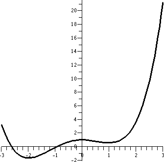 Example 0:
f(x)=(1/4)x4+(1/3)x3-x2+1
FUNC
We've seen this function several times. The function tells me that the
domain is all x. The positive coefficient, 1/4, on the top degree
term, x4, which has an even exponent, tells me that
limx-->+infinityf(x)=+infinity and
limx-->-infinityf(x)=+infinity. The precise range is
unclear (until we analyze the first derivative).
FUNC´
Now f´(x)=x3+x2-2x. This factors easily to
x(x+2)(x-1). There are critical numbers (where f´(x)=0 or doesn't
exist) at 0 and -2 and 1. The critical points (substitute the critical
numbers into the original function!) are at (0,1) and (-2,-5/3) and
(1,7/12). So now I can tell that the range of the original function is
[-5/3,inifnity) and (0,1) is a local max and (1,7/12) is a local min
and (-2,-5/3) is a global or absolute max. The function increases in
the intervals [-2,0] and [1,infinity) and decreases in the intervals
(-infinity,-1] and [0,1]. I can see this by looking at the "heights"
(the second coordinates) of the critical points and the limits at
+/-infinity found before. Or I can look at f´(x). Where is it
positive and where is it negative? The same answers will appear.
FUNC´´
So f´´(x)=3x2+2x-2. If we use the quadratic
formula then the roots are -1/3+/-sqrt(7)/3. These roots show
where the concavity of the graph of y=f(x) changes. For
(-infinity,-1/3-sqrt(7)/3] the graph is concave up. In the interval
[-1/3-sqrt(7)/3,-1/3+sqrt(7)/3], the graph is concave down. And
finally in the interval [-1/3+sqrt(7)/3,infinity) the graph is concave
up.
 Example 1: f(x)=e-x2
FUNC
I think that the domain is all x. The range? Maybe let's wait until we
analyze the derivative. But I do know that the exponential function is
never 0 and is always positive. I also know that
exp(large positive numbers) is large positive (exponential
growth) and exp(large negative numbers) is close to 0
(exponential decay). From this I can conclude that if
x-->+infinity or if x-->-infinity, then exp(-x2) will be
exp(large negative number) and therefore will be small. So
limx-->+infinitye-x2=0 and
limx-->-infinitye-x2=0. The x-axis
(with equation y=0) will be a horizontal asymptote.
FUNC´
We use the Chain Rule to compute f´(x)=e-x2(-2x).
The exponential function is never 0, therefore the only way this
formula can be 0 is when -2x=0. That's x=0, the only critical
number. Please notice that f(0)=e0=1, and therefore (0,1)
is the only critical point. Since the derivative is
e-x2(-2x) and the values of the exponential function
are always positive, I see that f´(x)>0 for x<0 and
f´(x)<0 for x>0. The function is increasing in the interval
(-infinity,0] and decreasing in the interval [0,+infinity). This also
agrees with the location of the point (0,1) on the graph and the
asymptotic behavior deduced above at +/-infinity. The point (0,1) is
a local and absolute maximum. The range of the function is (0,1].
FUNC´´
Since f´(x)=e-x2(-2x) we know (product rule
and Chain Rule) that
f´´(x)e-x(-2x)2+e-x2. Hey:
rewrite this as e-x2((-2x)2-2). Since the
exponential function is never 0 (and is always positive) the sign of
the second derivative depends on the sign of
(-2x)2-2=4x2-2. Let's see: this is 0 when
x=+/-[1/sqrt(2)]. It is positive when x>1/sqrt(2) and is positive
also when x<-1/sqrt(2). It is negative when
-1/sqrt(2)<x<1/sqrt(2). Therefore, as we say in math classes,
the graph will be concave up in the intervals (-infinity,-1/sqrt(2)]
and [1/sqrt(2),infinity) and concave down in the interval
[-1/sqrt(2),+1/sqrt(2)]. The inflection points occur at
(-1/sqrt(2),e1/2) and (1/sqrt(2),e1/2) (plug the
x-values into the original function!).
Note This isn't a miserable random function. If you ever do any
statistics, this is the function whose graph is the wonderful
"bell-shaped curve". The inflection points indicate dispersal from the
mean (in this case the mean is 0).
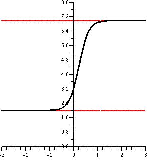 Example 2: f(x)=(6+7e5x)/(3+e5x)
FUNC The function is given by a formula which is a
quotient so we should be concerned about which x's given 0 on the
bottom. The bottom is 3+e5x. The values of the exponential
function are always positive so the bottom is always at least
3. Therefore the domain of this function is all numbers. The range
maybe is a bit mysterious, and we'll need some help from the
derivative. What about what happens as x-->+infinity? Here the
6+7e5x on the top is "dominated" by the big term,
7e5x. On the bottom as x-->+infinity, 3+e5x pays
no attention to the 3, and is essentially e5x. Therefore I
bet that limx-->+infinity(6+7e5x)/(3+e5x)=limx-->+infinity7e5x/e5x=7. Now
as x-->-infinity, the exponential term e5x-->0
("exponential decay") so that
limx-->-infinity(6+7e5x)/(3+e5x)=limx-->-infinity6/3=2.
Therefore the lines y=7 and y=2 are both horizontal asymptotes of
y=f(x), the first on the right and the second on the left.
FUNC´
Since
f(x)=(6+7e5x)/(3+e5x) I'll use the quotient rule to get the derivative. Therefore
         7·5e5x(3+e5x)-5e5x(6+7e5x)     105e5x+35e10x-(30e5+35e10x)
f´(x) = --------------------------- = --------------------------
              (3+e5x)2                        (3+e5x)2
and there is neat (?) cancellation so that
f´(x)=75e5x/(3+e5x)2. When is this equal
to 0? Well, it can only be 0 when the top is 0, but the top is a constant
multiplied by an exponential. Therefore the derivative is never 0.
And since we know that values of exp are all positive, we can deduce
that f´(x) is always positive, so that f(x) is always increasing (!).
FUNC´´
Since f´(x)=75e5x/(3+e5x)2, I compute
f´´(x)=
75(5)e5x(3+e5x)2-2(3+e5x)5e5x75e5x     75(5)e5x(3+e5x)-2·5e5x75e5x
--------------------------------- = ----------------------------
           (3+e5x)4                       (3+e5x)3
Here I've gotten rid of a factor of (3+e5x) on the two
pieces of the top and on the bottom. The top is:
75(5)e5x(3+e5x)-2·5e5x75e5x=75e5x(15+5e5x-10e5x)
The top is 0 exactly when 15-5e5x=0 or when
3-e5x=0 or when 3=e5x or when ln(3)=5x or when
ln(3)/5=x. Wow! For x<ln(3)/5 I bet (I'm helped by the
picture!) that the curve is concave up, and for x>ln(3)/5, it is
concave down. There is one inflection point.
Note This curve is what's called a logistic curve. It is
a curve which matches growth when there are limited resources. A small
chunk of this curve, say for x between -.4 and +.4, looks a bit like
exponential growth, but the global behavior has constant asymtotic
values. This is what happens when the slime mold (?) eats everything
around and exactly balances with the energy and nutrition coming in. I
hope you can imagine more interesting scenarios.
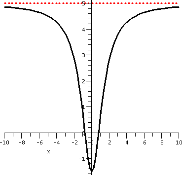 Example 3: f(x)=(5x2-3)/(x2+2)
I was not able to do this in class due to lack of time. So let me
outline what happens.
FUNC If f(x)=(5x2-3)/(x2+2), the bottom. x2+2, is
always at least 2. It is never 0. Therefore the domain of f(x) is all
x. As x-->+infinity, the dominant term in the top of the formula
defining f(x) is 5x2, and the dominant term in the bottom
is x2. Therefore the limit of f(x) as x-->+infinity
is 2. Since the x's all appear only with even powers, this graph is
symmetric with respect to the y-axis, and
limx-->-infinityf(x) is also 2. Therefore y=2 is a
horizontal asymptote of y=f(x) (on "both" sides!).
FUNC´
After some algebra, f´(x) turns out to be
26x/(x2+2>2. The bottom is always positive, so
the only way we could have a critical number is when the top is 0, and
this occurs only when x=0. The value of f(0) is -3/2. The derivative
is negative for x<0 and is positive for x>0. So (0,-3/2) is a
local (and absolute) minimum. The function is decreasing on
(-infinity,0] and is increasing on [0,infinity).
FUNC´´
Much more algebra gives the following for
f´´(x):
-26(3x2-2)/(x2+2)3. Now
f´´(x)=0 when 3x2-2=0 so this is when
x=+/-sqrt(2/3). There are two inflection points, and f(x) is
concave up in the interval between them, and concave down
elsewhere. If you look at the graph you'll see that this
information can be confirmed there.
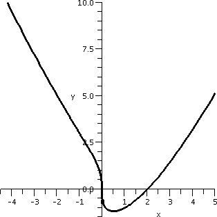 Example 4: f(x)=x1/3(x-2)
Again, I was not able to do this in class due to lack of time. One
"feature" of this function is that it isn't differentiable at all
x. So it has something interesting separating it from the other
examples. Also even plotting the darn thing with a machine was more
difficult, since most of the standard plotting devices sort of assume
that curves will be smooth. I had the machine draw the
picture shown with some deviousness.
FUNC
The nasty (or interesting?) thing here is the power of
one-third. Since 3 is odd (!!) the domain of x1/3 is all
numbers, and therefore the domain of f(x) is all numbers. Another way
of writing f(x) results from distributing the multiplication:
f(x)=x4/3-2x1/3. If x is really huge in
magnitude (either positive or negative) then I bet the highest power
"rules". So f(x) when x is huge is just about x4/3. the
fourth power of the cube root makes things positive. I bet that as
x-->+infinity, f(x)-->+infinity, and as x-->-infinity,
f(x)-->+infinity.
FUNC´
The derivative, after some algebraic "massaging", turns out to be
[2(2x-1)]/[3x2/3]. Hey! What are the critical numbers?
Well, they are either where f&!80;(x)=0 (and that is when 2x-1=0 so
x=1/2) or when x=0 (because there is a
power of x in the bottom and we can't divide by 0). Actually, the
domain of f´(x) is all non-zero numbers. The original function
f(x) is not differentiable at x=0. Since f(0)=0 and
f(1/2)=[1/21/3](-1/2), I see that f(x) has a local and
absolute minimum at x=1/2. At x=0, the critical point is neither a
maximum nor a minimum. The sign of f´(x) is negative on both
sides of 0, so f(x) decreases on both sides of 0.
FUNC´´ The second
derivative turns out to be
4(x+1)/[9x5/3]. For x<-1, this is a negative number
divided by a negative number, so f´´(x)>0 and f(x) is
concave up. For x between -1 and 0, the top "changes" sign to
positive, but the bottom is still negative: f´´(x)<0 and
f(x) is concave up. For x>0, both the top and bottom of the formula
4(x+1)/[9x5/3] are positive, so the quotient is
positive. Now f´´(x)>0 so f(x) is concave up.
There are two inflection points.
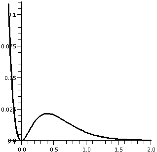 Example 5: f(x)=x2/e5x
FUNC Remember that the exponential function is always
positive, so the bottom (denominator) of the formula defining this
function is never 0. Therefore the domain is all numbers. Notice that
as x-->-infinity, the bottom, e5x-->0 and the top,
x2-->+infinity. f(0)=0, and the fraction is always
non-negative. These facts together show that the range of f(x) is all
non-negative numbers. The hard thing to decide is what happens as
x-->+infinity. The derivative can help with this.
FUNC´ Since
f(x)=x2/e5x, I know that
f´(x)=
2xe5x-x2e5x5    (2x-5x2)
------------ = --------
  (e5x)2          e5x
which we
get by factoring out and dropping one e5 from all the
terms, top and bottom. Where is this 0? We need only consider the top
for this: 2x-5x2=0 means x(2-5x)=0 so this means x=0 or
x=2/5. These are the critical numbers. Now substitute into f(x) and
get the critical points:
(0,0) and (2/5, (4/9)/e2)
Therefore (0,0) is a relative and absolute minimum of f(x), and the
other critical point is a relative max. f(x) decreases in the
intervals (-infinity,0] and [2/5,infinity) and f(x) increases in the
interval [0,2/5].
But what happens to f(x) as x-->+infinity? The graph shown above and
the calculus work so far don't entirely convince me that I
know. Maybe as x-->+infinity, f(x) decreases to .000345 (it
doesn't, but maybe it could. Well, here is a trick to show you what
happens, or maybe to convince you that f(x) does actually -->0
as x-->+infinity. Let me pull a little bit of the exponential away on
the bottom. I'll write things like this:
  x2      x2      1
----- = ----- · ----
  e5x     e4x     ex
The factor x2/e4x looks more or less like
x2/e5x: in particular, for large enough x's this
is positive and decreasing. The other factor, 1/ex must
-->0 as x-->+infinity. So when x gets large, we can write
x2/e5x as a product of something that's at worst
bounded multiplied by something that -->0. So the limit of
x2/e5x must be 0 as x-->+infinity. And the
x-axis (with equation y=0) is a horizontal asymptote of y=f(x).
Comment I'll show you a different way
to do this next time. And maybe that way will be more understandable,
too. It will certainly be more computable.
FUNC´´
The "finer" (?) structure of the graph may be revealed by studying the
second derivative. Since
f´(x)=(2x-5x2)/e5x,
f´´(x)= (2-10x)e5x-5e5x(2x-5x2) (2-10x)-5(2x-5x2)
----------------------- = ------------------
(e5x)2 e5x
The bottom is always positive, so the top will determine the sign of
the second derivative and where the second derivative is equal to 0.
The top "simplifies" to 25x2-20x+2. The roots of the top
(using the quadratic formula) are
-(-20)+/-sqrt[((-20)2-4(25)2] all divided by 2(25). This is
(2/5)+/-(1/5)sqrt(2). So there will be one inflection
point between the minimum and the relative maximum, and one inflection
point to the right of the relative maximum. This does agree with the
graph. y=f(x) is concave up on the intervals
(-infinity,(2/5)-(1/5)sqrt(2)] and [(2/5)+(1/5)sqrt(2),+infinity) and
it is concave down on the interval
[(2/5)-(1/5)sqrt(2),(2/5)+(1/5)sqrt(2)].
I handed out a take-home semi-exam.
Wednesday, July 19
We discussed some graphs from homework problems. I don't have the
record here, but please look at the answers to the take-home semi exam.
Then I asked students to work together and discuss some data. Several groups reported on
each data collection, and tried to expression in words and symbols
what the data showed. ALso, we tried to draw a convincing and
appropriate graph for each data set. The data sets were chosen to
describe some variable changing with respect to another variable. The
changes themselves had some changes in time, which, in the cases
displayed, had some meaning. Therefore I wanted to show that a
function and it derivative and its second derivative could be
important and useful in describing phenomena.
Data set #1
Here is 1931 inflation data. C(t) is the consumer price
index. Describe what you can about C´(t) and
C´´(t). Describe the behavior of $C(t)$ in words. Draw a
plausible and qualitatively correct graph of C(t).
| Inflation rate |
|---|
| January | February | March |
April | May | June |
| -7.02% | -7.65% | -7.69% |
-8.82% | -9.47% |
-10.12% |
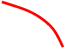 The inflation rate is, essentially, already C´(t). So C´(t)
is negative and decreasing (remember to use both magnitude and sign
to think about this). Therefore C´´(t)<0. As we move
from left to right (time increases) the slope of C(t) is decreasing.
Data set #2
Here is 1998 inflation data. C(t) is the consumer price
index. Describe what you can about C´(t) and
C´´(t). Describe the behavior of C(t) in words. Draw a
plausible and qualitatively correct graph of C(t).
| Inflation rate |
|---|
| May | June | July |
August | September | October |
| 1.69% | 1.68% | 1.68% |
1.62% | 1.49% |
1.49% |
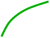 Again, the inflation rate is, essentially, already C´(t). So C´(t)
is positive and decreasing (remember to use both magnitude and sign
to think about this). Therefore C´´(t)<0. As we move
from left to right (time increases) the slope of C(t) is decreasing
although it is certainly always positive.
Data set #3
Here is 1965 inflation data (enough already!). C(t) is the consumer
price index. Describe what you can about C´(t) and
C´´(t). Describe the behavior of C(t) in words. Draw a
plausible and qualitatively correct graph of C(t).
| Inflation rate |
|---|
| January | February | March |
April | May | June |
| 0.97% | 0.97% | 1.29% |
1.62% | 1.62% |
1.94% |
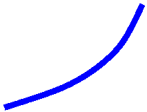 The inflation rate is, essentially, already C´(t). So C´(t)
is positive and increasing: this is a real data set (as far as I know)
so it isn't "perfect" -- it is {mostly|sort of} increasing!
Therefore C´´(t)>0. As we move
from left to right (time increases) the slope of C(t) is increasing.
Data set #4
Salt (NaCl, sodium chloride) has a saturation amount (the most salt
that can be dissolved) which varies with temperature. Here is the
amount of salt in grams which can be dissolved in 100 mL (milliliters)
of water (H2O) at various temperatures:
| Saturation amounts as a
function of oC |
|---|
| 0 | 10 | 20 |
30 | 40 | 50 |
| 35.7 | 35.8 | 36.0 |
36.3 | 36.6 | 37.0 |
Suppose S(c) is the saturation amount as a function of the
temperature. Describe what you can about S´(c) and
S´´(c). Describe the behavior of S(c) in words. Draw a plausible
and qualitatively correct graph of S(c).
 So this is maybe simpler data (!) than the inflation rate. This
function is increasing (these numbers are a table of the function, not
the derivative!). The derivative is sort of the rate of change of the
numbers, so from 0 to 10 we get .1 (grams per 100 mL per 10 degrees),
and then .2 and then .3 and then .3 and then .4. So certainly the
saturation amounts are increasing: S´(c)>0. The rate of
increase is, itself, generally increasing, so that
S´´(c)>0. I guess the qualitatively correct graph which
best matches this data is the same one drawn before.
I didn't get the fourth possibility, I think. The fifth data set given
in the handout has, more or less, very little change in the
derivative. The "curve" is decreasing but the rate of decrease is
rather steady.
Discussion of concavity
Here are some pictures I drew. I emphasized that I wasn't
proving that the pictures (logically) identified the same
collections of curves: this was true, but the equivalencies were not
too easy to see.
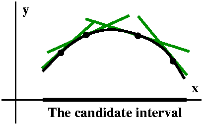
| A function is concave up on an interval if |
Secant lines drawn through any pairs of points on the graph (in
the interval!) always lie above the graph between the two points.
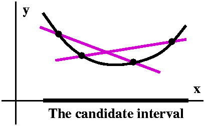
|
Tangent lines to the graph at points in the interval always lie
below the graph on the interval.
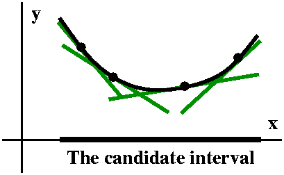
|
| A function is concave down on an interval if |
Secant lines drawn through any pairs of points on the graph (in
the interval!) always lie below the graph between the two points.
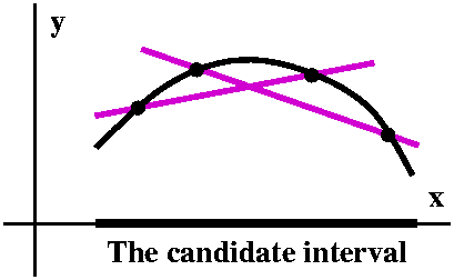
|
Tangent lines to the graph at points in the interval always lie
below the graph on the interval.
|
If the second derivative of a function is positive in an interval,
then the first derivative of the function is increasing is increasing
in that interval. Then, as x "moves" from left to right, the slope of
the tangent line to the graph of the function rotates
counterclockwise. The result is that the curve bends "up", and is
concave up. If the second derivative is negative, the result is the
grpah of the function is concave down. It is useful to notice this,
and also to notice that there need not be any connection
between {in|de}creasing behavior and concavity.
| |
If f´´(x)>0
in an interval |
If f´´(x)<0
in an interval |
|---|
If f´(x)>0
in an interval |
The function is increasing and the graph is concave up in that
interval.
 |
The function is increasing and the graph is concave down in
that interval.
 |
If f´(x)<0
in an interval |
The function is decreasing and the graph is concave up in
that interval.
 |
The function is decreasing and the graph is concave down in
that interval.
 |
|---|
Points on the graph where the concavity changes are called
inflection points. A bunch of examples may be useful now, or
they may just increase confusion. Oh wel.
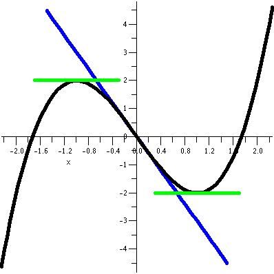 f(x)=x3-3x
One good example or two might be useful to
continue the confusion. If f(x)=x3-3x, then
f´(x)=3x2-3=3(x-1)(x+1). There are critical numbers at
+/-1, and (using f(x) to get the second coordinates) the critical
points are (-1,2) and (1,-2). The first derivative's sign changes at
-1 and +1, and the function is increasing in the intervals
(-infinity,-1] and [1,infinity). The function is decreasing in the
interval [-1,1]. Now f´´(x)=6x. So when x>0, the graph is
concave up because f´´(x) is positive, and when x<0, the
graph is concave up because f´´(x) is negative. The point
(0,0) is an inflection point. All four of the behaviors in the chart
above can be obersed in different parts of this graph: concave up and
increasing in [1,infinity), concave up and decreasing in [0,1],
concave down and decreasing in [-1,0], concave down and decreasing in
(-infinity,-1].
Notice the tangent line segments, please
There are two pieces of the tangent lines at the local max and the
local min. They are horizontal. The local picture is fairly easy to
understand. But the tangent line through (0,0), which is y=-3x, is
less easy to understand. It "looks" tangent to the curve, but on one
side of the curve it is on top and on the other side of the curve it
is on the bottom. At an inflection point, the tangent line cuts
through the curve. This realization may be a bit uncomfortable!
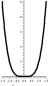
f(x)=x4
The graph of f(x)=x4 looks like a sort of parabola which is
steeper when |x| is large and flatter when x is near the origin..
Here f´(x)=4x3, and (0,0) is a critical point. Even
though f´#180;(x)=12x2 and f´#180;(0)=0, the
point (0,0) is not an inflection point! The curve is concave up
everywhere.
We are facing the converse of an implication
again, and the converse of a true implication need not necessarily be
correct. Here the implication is that if
(x0,f(x0)) is an inflection point, and if
f´#180;(x0) exists, then f´#180;(x0)
must be 0. That's true. But the other way around is not always
correct.
|
|
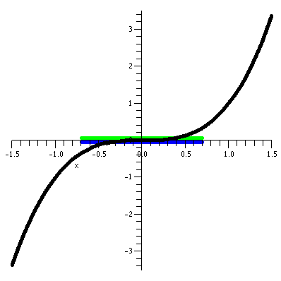
f(x)=x3
Here f´(x)=3x2, and (0,0) is a critical point. We
compute f´#180;(x)=6x so the second derivative is positive when
x>0 (so the graph is concave up there) and the second derivative is
negative when x<0 (so the graph is concave down there). Therefore
the point (0,0) is not an inflection point. Notice that the
horizontal line at the origin is the tangent line because (0,0) is a
critical point, and that line crosses the graph because (0,0) is an
inflection point. The critical point is neither a local maximumum nor
a local minimum.
|
|
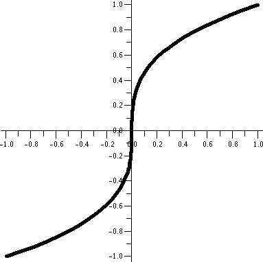
f(x)=x1/3
This function increases for all x. The origin is a critical point, but
this is because the derivative does not exist at the origin (the
geometric tangent line is vertical there, and vertical lines have no
slope). The derivative for x not 0 is given by (of course!)
f´(x)=(1/3)x-2/3 and for x not 0, the second
derivative has the formula f#180;´(x)=-(2/9)x-5/3. You
can check the signs of the first and second derivative. f(x) is
increasing for all x. f(x) is concave up for x<0 and f(x) is
increasing for all x. f(x) is concave down for x>0.
|
|
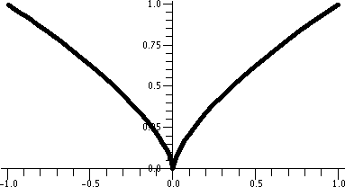
f(x)=x2/3
Finally, here is an example of what is called a cusp (the
pointy behavior at the origin). Since f´(x)=(2/3)x-1/3
for x not equal to 0, the function decreases to the left of 0 and
increases to the right of 0. And
f#180;´(x)=-(2/9)x-4/3 for x not equal to 0. The
function is concave down for x<0 and it is concave down for x>0.
|
|
Tuesday, July 18
We did three or four more graphs. Please look at the answers to the
take-home semi exam for work similar
to what was done in class. I tried to emphasize that Step 0 for me under any
realistic circumstances was using a graphing device whenever possible:
a graphing calculator or ... something! Then I would try to get
information about the function in Step
1. And the derivative would be used in Step 2. Later we'll learn
Step 3.
One beauty (!) was f(x)=(1/3)x3-(1/5)x5, which
had rather complicated behavior near the origin.
Derivatives of derivatives are frequently called higher
derivatives. We computed some "higher" derivatives.
| The function | x8
| 5sin(3x) | 44e9x | 1/x3 |
Notation
Usually f(x), but sometimes (!) seen as the zeroth derivative:
f(0)(x) |
|---|
|
|
What to call it
In physics problems, f(x) might represent position or displacement on
a sort of road. There's an origin, or start. To the left of the
origin, the position would be labeled with a minus sign, and to the
right, with a plus sign. So the sign indicates the direction of the
distance to the origin. The first derivative is velocity. A
plus sign means movement to the right, and a minus sign means movement
to the left. "Speed" is velocity without the sign.
|
|
| The first derivative
| 8x7
| 5·3cos(3x)
| 44·9e9x
| (-3)x-4
| This is f´(x) or f(1)(x)
or dy/dx or y´.
|
|---|
|
|
What to call it
In physics problems, f(x) might represent position or displacement on
a sort of road. There's an origin, or start. To the left of the
origin, the position would be labeled with a minus sign, and to the
right, with a plus sign. So the sign indicates the direction of the
distance to the origin. The first derivative is velocity. A
plus sign means movement to the right, and a minus sign means movement
to the left. "Speed" is velocity without the sign.
|
|
| The second derivative
| 8·7x6
| -5·32sin(3x)
| 44·92e9x
| (3·4)x-5
| This is f´´(x) or f(2)(x)
or d2y/dx2 or y´´.
|
|---|
|
|
What to call it
In physics problems where f(x) represents position,
then the second derivative is acceleration. Here the plus sign
would be velocity increasing and the minus sign would be velocity
decreasing.
Warning If velocity changes from -4 to
-2, then acceleration would be positive. If velocity changes from 2 to
4, then acceleration would also be positive. In both cases, velocity is
increasing. So things can be a bit tricky.
|
|
| The third derivative
| 8·7·6x5
| -5·33cos(3x)
| 44·93e9x
| -(3·4·5)x-6 | This is
f´´´(x) or f(3)(x)
or
d3y/dx3 or y´´´.
|
|---|
|
|
What to call it
In physics problems, if f(x) represents position or
displacement, then I have heard that the third derivative is called
jerk. I don't think I've ever really heard that term used
much, except when a student is referring to ...
|
|
| The 78th derivative
| 0
| -5·378sin(3x)
| 44·978e9x
| (3·4·5·6·...·79·80)x-81
| This is f(78)(x) or d78y/dx78.
I've never seen more than two or three primes in a row!
|
|---|
|
|
What to call it
I don't know any neat name for a derivative as "high" as
this. It is the 78th derivative, in the unlikely event that
you need to talk about it!
|
|
Demystification and pattern recognition
I wanted to compute the entries in this table partly to "demystify"
(?) the process, but also to ask people to look for patterns. In the
case of the first function, a polynomial, differentiating pushes down
the highest power by 1 until that highest power gets to be 0 (so the
result then is a constant). All further, higher, derivatives are 0.
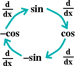 What about 5sin(3x)? Here the 5 just gets carried along, but no higher
derivative is going to be the zero function. Each derivative will
"spit out" (due to the Chain Rule) a 3 to multiply the result. But
what about the other parts of the function? Well sine and cosine do a
dance (?!) when differentiated. The dance steps are pictured to the
right. It is sort of a waltz (forget about the 3x inside for a second,
please). Every fourth step brings us back to where we were. So if we
wanted the 78th derivative of sine, we would divide 78 by
4. This would be 19: but not exactly -- there would a be a remainder
of 2. This means that the 78th derivative waltzes around
this figure 19 times, and then does two more steps, so that the result
would be -sine. Wow (maybe). The result would still have the 5
and 78 of the 3's multiplying and the darn 3x inside the function. But
the waltz makes the computation easy. (I don't want to make things too
darn easy: the derivatives of tan have no simple structure.)
The exponential function is your friend. If sine and cosine's
derivatives waltz in a 4-step pattern, then, oh my goodness, what
exponential does when differentiated is jump up and down, since
exp´(x)=exp(x) (the derivative of e-to-the is e-to-the!). OF
course the 44 is carried along as a multiplicative constant, and each
differentiation brings out another multiplication by 9.
1/x3 is x-3. Differentiation follows the power
rule, but because we begin with a negative integer, we never "get" to
0. Actually we just keep going down and down and down. The integers
get larger in absolute value and come out "in front" at each
differentiation. The sign result alternates between + and -, and the
odd-numbered derivatives get the minus sign, while the even numbered
derivatives get the plus sign. If you desperately needed a compact way
to write the derivatives, there is notation available, using the
factorial sign (the surprise mark: !) but I am not too interested in
efficiency here. I would like you to see the patterns. Higher
derivatives for "simple" functions aren't too hard to compute.
I wanted to show a use of higher derivatives. The simplest use might
be from a physical problem. So here is one.
Abrupt stop to a car
A car is speeding along at 60 miles per hour (which I remember from
high school is 88 ft/sec). Suppose the car hits a wall and comes to a
stop in a tenth of a second. If the deceleration is assumed to
be constant, what is the deceleration? If you can do such analysis,
maybe you could be an expert witness in car accident cases, and
make big bucks. Ooops, sorry: maybe you could help that the correct
side wins in the court case.

Here a(t)=K, a constant by assumption. I'll use the letter K for a
constant. So I know that a(t)=K, and then by antidifferentiating,
v(t)=Kt+C. But v(0)=88. I'm using distance measured in feet and time
measured in seconds. Thus v(t)=Kt+88. Since v(1/10)=0, we know
K(1/10)+88=0, so that K=-880 ft/sec2. The "acceleration" of
gravity is about 32 ft/(sec)2. So let me compare this
deceleration to gravity, an interesting and horrifying comparison. Notice that
880/32 is 27.5: so this deceleration presses the "contents" of the car
(the passengers!) with a force twenty-seven and a half times that of
normal gravity. Imagine even briefy your weight multiplying by that
factor. The consequences are most unpleasant. A chapter in a book I
read, Stiff: The Curious Lives of Human Cadavers by
Mary Roach, discusses this situation in detail. Those of you
interested in becoming doctors might want to read this book. But if
you were holding a 10 pound baby in your arms, that baby would, for a
short time, seem to "weigh" 275 pounds. Holding such a load, even for
a very short time, seems perilous. I think the child would be released
at its peril. Indeed, even if you are a big, strong "guy", with
weight, say, 200 pounds, could you hold yourself safely when you might
seem to weigh more than two tons? (27.5·200=5,500)
Monday, July 17
I wrote the Mean Value Theorem again.
Example 1: distance traveled and speed
Suppose I told you that I have driven on a straight road for two hours
with my speed (really, darn it, velocity!) between 40 and 60 miles per
hour. If we assume that my travel is differentiable (I would not want
to travel non-differentiably, because the times when the derivative
didn't exist would be most unpleasant!) what can be said about the
distance traveled? If f(t) is the position at time t in terms of miles
from the origin (of whatever road I am on) then according to the MVT,
f(time2)-f(time1)/(time2-time1)=f´(some time in between).
Here
the information I have is that the elapsed time,
time2-time1, is 2 hours (time will be measured
in hours, and distance in miles). And I told you that my
velocity is always between 40 and 60, so 40<f´(some time in between)<60. Therefore
the equation above becomes
40<f(time2)-f(time1)/(2)<60
so that (multiplying by 2) we get
40·2=80<f(time2)-f(time1)<60·2=120.
I think that most children aged, maybe 10 or 12 and above will come up
with the same result. Do they have the MVT "wired in" to their brains?
I don't know. I don't know how a child or an adult or any person
(including myself!) thinks. But I wanted to go through this as part of
the effort to convince you that the MVT is a natural part of thought,
at least in certain physical situations.

Example 2
This will be more like something in a math course, so we will be
happy. Suppose f(x)=sqrt(5x600+4). I can compute (the darn
function is arranged so that the computation is easy) f(0)=2 and
f(1)=3. What can one be said about f(.3781334)? This maybe can also be
thought through without needing "higher math" but I want to organize
your head a bit. Well, f(x) is defined by a (relatively!) nice
formula. I bet it is continuous wherever it is defined. And, actually,
since the power inside is even, the "stuff" inside the square root
will be non-negative, actually positive (at least 4) so the domain of
f(x) is all x. Hey, what do we know using "continuity" about
f(.3781334)? The answer is, not very much. If the only
information is f(0)=2 and f(1)=3 and continuity of f(x), there
is no restriction on f(.3781334). Look at the darn graphs. But:
If f(x)=sqrt(5x600+4) then
f´(x)=(1/2)(5x600+4)-1/2(5·600x599. Hey,
maybe this is a complicated "thing". But the only information I want
right now is the sign of this complicated thing when x is in
the interval [0,1]. And getting the sign is easy. The only minus is in
the exponent (which forces something "downstairs") so I know that
f´(x)>0 in [0,1]. This means, according to a result following
the MVT, that f(x) is increasing in this interval, so I know
that f(0)=2<f(.3781334)<f(1)=3. The desired value of f(.3781334)
is between 2 and 3. I will admit that this isn't very much but it is a
heck of a lot more than knowing nothing! So the MVT gives us
more information.
| If |
then |
The graph looks like ... |
|---|
| f´(x) is positive on an interval |
f(x) is increasing on the interval |
As x "moves" from left to right on the horizontal axis,
the point (x,f(x)) moves "up" on the graph of y=f(x). |
| f´(x) is negative on an interval |
f(x) is increasing on the interval |
As x "moves" from left to right on the horizontal axis,
the point (x,f(x)) moves "up" on the graph of y=f(x). |
I applied these ideas to the graph of
f(x)=(1/4)x4+(1/3)x3-x2+1.
Here f´(x)=x3+x2-2x. This is an example
from a calculus course so it factors neatly, and
f´(x)=x(x+2)(x-1). The derivative is 0 at x=0 and x=-2 and
x=1. It isn't too hard to figure out where the derivative is positive:
in the intervals (-2,0) and (1,infinity). There the function is
increasing. The derivative is negative in the intervals (-infinity,-2)
and (0,1) so the function is decreasing in those intervals. We already
this function maybe too well (anything from an exam is such a
thing). Let me try to look at something new.
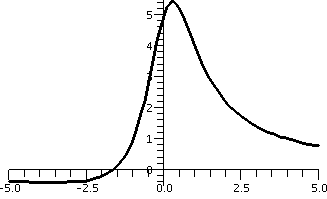 f(x)=(3x+5)/(x2+1)
I look at this function and think about its domain: all x (because the
bottom is never 0 since x2≥0 so it must be at least 1).
I also see that as x-->+infinity, the top is mostly 3x and the bottom
is x2, so the function is almost 3/x and this -->0 as
x-->+infinity. A similar analysis shows that f(x)-->0 as x-->-infinity
also. What about bumps, etc.? A good hint is gotten by looking at a
mechanically produced graph of this function, as shown to the right. I
can get more precise information from the derivative.
We computed f´(x). We used the quotient rule and were
careful. The result, after some algebraic effort, was
(-3x2-10x+3)/(x2+1)2. I am interested
in the sign of f´(x) and I notice that the bottom is always
a square, so it is always positive (it isn't 0 -- we saw that
earlier). So let's look at the top:
-3x2-10x+3
The roots of this quadratic (using the quadratic formula) are
-5/3+/-sqrt(34)/3. These numbers are about -3.61031 and 0.27698.
We can then substitute them back into the original function, f(x).
The results are the points (-3.61031,-.38784) and (0.27698,1.37610). I
think one is the top bump and the other is the lower bump.
Here are my conclusions, which I think I'd not be very sure about
without using calculus (because, darn it, the "pictures" produced by
machines can be deceptive and sometimes even incorrect!):
The range of f(x) is [-.38784,,1.37610].
f(x) is increasing in the interval [-3.61031,0.27698].
f(x) is decreasing in each of these intervals:
(-infinity,-3.61031] and [0.27698,infinity).
I'll be honest: I doubt many students in Math 135 will need to know
even these details about such a function. But if you've go to know,
calculus is the best way to be sure you are correct.
Thursday, July 13
We used the MVT to deduce a result about {in|de}creasing
functions. First let's state the definitions:
Increasing
A function f(x) is increasing on an interval I if for any pairs
of numbers x1 and x2 in I, if
x1<x2, then
f(x1)<f(x2).
Decreasing
A function f(x) is increasing on an interval I if for any pairs
of numbers x1 and x2 in I, if
x1<x2, then
f(x1)>f(x2).
It could be very difficult to verify either of these
definitions directly, since it seems that we'd have to take every pair
of points, and check some inequalities for all of them. Well, the MVT
allows a much easier method.
f´(x)>0 implies f(x) increasing on an interval
f´(x)<0 implies f(x) decreasing on an interval
Well, suppose f´(x) is positive on I, and x1 and
x2 are two points on I with
x1<x2. Then by MVT,
f(x2)-f(x1)
----------- =f´(somewhere in between)
   x2-x1
If I know that the derivative values are always positive, and if I
know that x2-x1 is positive (which is true
if x2>x1) then the equation isSIGN NOT KNOWN
-------------- = POSITIVE #
POSITIVE #
so that in fact, the SIGN NOT KNOWN, which is the term
f(x2)-f(x1), must also be positive. But then
f(x2)>f(x1). We have proved that f(x)
must
be increasing on an interval where the derivative is positive.
A similar verification can be applied to the case of negative
derivatives. The usefulness of all this is determining whether
functions are positive or negative is usually much easier than
checking (directly) whether they are increasing or decreasing.
I applied this to analyze a function like
8e-3x+5e4x. Here
f(x)=8e-3x+5e4x
then f´(x)=-24e-3x+20e4x. Let's see where
this derivative is 0:
-24e-3x+20e4x=0 happens when
20e4x=24e-3x. I'll divide by 20 and multiply by
e3x using the exponential rules. The
result is e7x=24/20=6/5. Taking ln's undresses the exp's,
so we know 7x=ln(6/5) and x=(1/7)ln(6/5). What now? I know that
limx-->+infinityf(x)=+infinity, because the e4x
term gets very large and the other term is positive. Similarly,
as x-->-infinity, the e-3x in f(x) gets large.
I think that f´(x)>0 for x>(1/7)ln(6/5). I know the
derivative can't equal 0, because we found the only number where it
equals 0. The derivative can't be negative in that region,
because otherwise (Intermediate Value Theorem) it would have to be
0 (not possible!) because it would have both positive and negative
values. The logic is a bit extended but I hope you can follow
it. Similarly, f(x) is decreasing for x<(1/7)ln(6/5).
The minimum value of the function is f((1/7)ln(6/5)). All
other values are larger. I don't really know how to see this easily
without calculus.
The first formal 80-minute exam was given.
Wednesday, July 12
y=2|x|+4|x-3|
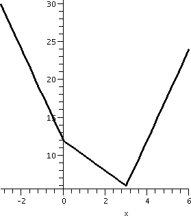 Various computational devices would produce something like what is
shown to the right as a graph of f(x)=2|x|+4|x-3|.
Why is this picture correct? I believe it is, but is there some way of
getting reassurance about the correctness? I ask this for several
reasons:
- Sometimes a graphing device may not be convenient to use or available.
- Sometimes a graphing device may actually be wrong.
- Sometimes a graphing device may operate "correctly", according to
its design and instructions, but the result may be misleading. (It
isn't too hard to find formulas that may give bad results on the
graphing calculators in common use.)
- Sometimes a formula may be so darn complicated (not true here!)
that a graphing device may actually not be able to cope with the
complications (I'll give some examples later of this.
So what should we expect of f(x)=2|x|+4|x-3|?
Well, this
function is made up of several pieces of the absolute value function,
which we analyzed earlier in the
course. Some of the facts discussed there will be relevant
here. First, the algebraic definition of absolute value:
          / Number if Number≥0
|Number|=<
          \ -Number if x<0
.
Second, we learned some qualitative things about the absolute
value function which have important implications for the graph of the
function: the function is continuous for all numbers, so the graph
will be unbroken, and have no jumps or breaks. The function is
differentiable everywhere except at the origin. To the
left of the origin, the function has derivative -1 (the graph is part
of a straight line with slope -1). To the right of the origin, the
function has derivative +1 (the graph is part of a straight line with
slope +1). At the origin, the function is not differentiable, and the
graph shows a corner.
What can I expect about this f(x), which is given by the formula
2|x|+4|x-3|? It is the sum of continuous functions, so f(x) should
also be continuous. The graph should have no breaks or jumps. The
function has |x| in it, and also |x-3|, which "translates" or shifts
the absolute value function 3 units to the right. I'd expcet that
there should be nice behavior away from 0 and 3, where nice now means
differentiable -- there should be a tangent line.
Well, the algebra can show some of this. If x<0, then |x| is
-x. What about |x-3|? If x is negative, x-3 makes it "more negative",
so |x-3| is -(x-3). therefore if x<0, f(x), which is
2|x|+4|x-3|, will be 2(-x)+4{-(x-3)}. I fouled this up in class, so
let me be careful here: f(x)=-2x-4(x-3)=-6x+12.
Now as x "moves" to the right (so x>0) |x| changes its
description. Notice, please, that |x-3| does not change description
"immediately". What do I mean? For example, if x=1,|x-3| becomes
|1-3|=|-2|=2. So if x<3, x-3<0, and |x-3|=-(x-3). Therefore, if
0<x&;t3, f(x)=2|x|+4|x-3|=2(x)+4{-(x-3)}=2x-4x+12=-2x+12.
What happens when x>3? Then x-3 is positive, and |x-3|=x-3. x
itself is of course positive, so |x|=x. And
f(x)=2|x|+4|x-3|=2(x)+4(x-3)=2x+4x-12=6x-12.
f(x) defined piecewise
Here is another definition of f(x), exactly equivalent to the
original.
     / -6x+12 if x<0
f(x)=< -2x+12 if 0≤x≤3
     \  6x-12 if 3<x
What can I learn with this piecewise definition? Well, I can see that
the graph of f(x) is actually made of parts of three lines. To the
left of 0, the graph of f(x) is part of a line with slope -6. Between
0 and 3, the graph is part of a line with slope -2, still negative but
"shallower" than the other segment. Finally to the right of x=3, the
graph is part of a line with slope 6, tilted up. Do the pieces of
the lines connect? Well if I consider -6x+12 as x-->0- the
result is 12. And -2x+12 as x-->0+ also gives 12. Hey:
these two pieces connect. And, around x=3, if we look at -2x+12
as x-->3-, the result is -2(3)+12=6, while if we look at
6x-12 as x-->3+, the result is 6(3)-12=18-12=6. These
pieces are also connected. Hey: the graph has one piece, and the
function is continuous.
What about the derivative? The algebra should reinforce the
picture. The infinitesimal rate of change of f(x) for x<0 is
the rate of change of the formula -6x+12. I think that rate of change
is -6. Between 0 and 3, the rate is -2, from the formula -2x+12. What
happens "at" 0? There is no one number describing this rate of
change. The derivative does not exist. The function is not
differentiable at x=0. A similar thing happens at x=3. So here is a
description of the function f´(x). First, this function has the
following domain: all real numbers except for 0 and 3. And when
x is in the domain of f´(x), we have
       / -6 for x<0
f´(x)=< -2 for 0<x<3
       \  6 for 3<x
I hope now that you can see that "algebra"
has confirmed the details of the picture of y=f(x).
y=x3-2x2+x+5
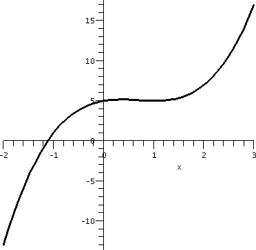 Now let me look at f(x)=x3-2x2+x+5. This is
"easy" (well, maybe). There is one nice algebraic formula defining
f(x). The domain for this polynomial is all real numbers, and
polynomials are continuous and polynomials are differentiable. In
fact, look, f´(x)=3x2-4x+1, so the function sure is
differentiable. I should expect that the graph will have no jumps --
it will have one piece. I should expect that the graph will be a nice,
smooth curve, with a neat tangent line at every point. So far, the
picture to the right should be further evidence of these assertions.
But there's some finer structure to the picture which I've not
discussed. The curve seems to wiggle in some fashion. How can I
be more precise about the wiggling? How can I analyze this wiggling?
The wiggling really has to do with the rate of change, so maybe I
should look at f´(x)=3x2-4x+1 more closely. Well, I
was lucky (really!) when I specified f(x), and I did not expect that
f´(x) would have a nice algebraic property. I thought that I'd
need the quadratic formula for the roots of f´(x): that would
mean considering
-(-4)+/-sqrt{(-4)2-4·3·1 (all divided by
2·3. Hey, this is
[4+/-sqrt(16-12)]6=[4+/-sqrt(4)]/6=[4+/-(2)]/6. The roots are 1/3 and
1. Or I could just have "observed" that
f´(x)=3x2-4x+1=(3x-1)(x-1).
Consequences of f´(x)=(3x-1)(x-1)
I know that the derivative is 0 when x=1. But
f(1)=13-(2)12+1+5=1-2+1+5=5. So the graph of the
function should have a horizontal tangent at (1,5). Also I know that
the derivative is 0 when x=1/3. And
f(1/3)=(1/3)3-(2)(1/3)2+(1/3)+5=
(1/27)-(2/9)+(1/3)+5=(1/27)-(6/27)+(9/27)+3=5{4/27}. This is about
5.148. And there's a horizontal tangent at (1/3,5.148)
When I first wrote the polynomial and had a machine graph it, the
bumps were not totally "obvious" to me. The initial
resolution of the graph wasn't very fine, and I didn't "see" the one
bump higher than the other bump. I just saw a sort of wiggle. With the
additional evidence of the algebraic analysis, I think I "see" that
the graph goes up (as a point moves on the graph from left to right)
until x=1/3, and then the graph goes down until x=1, and then finally
up once again. This is much more detailed information than the rather
casual first graph I saw. For example, I now believe that f(.47) is
greater than f(.55): I maybe could not have made such an assertion
with confidence before the analysis.
Definition #1
A function f(x) has a relative maximum at c if
- The domain of f(x) includes an interval that c is
inside. (So endpoints of domains can't be relative maxes).
- In that interval, f(c)>=f(x) for all x's in the interval. (So
f(c) must be so smaller than all the f(x)'s in the interval.)
Definition #2
A function f(x) has a relative minimum at c if
- The domain of f(x) includes an interval that c is
inside. (So endpoints of domains can't be relative maxes).
- In that interval, f(c)<=f(x) for all x's in the interval. (So
f(c) must be no larger than all the f(x)'s in the interval.)
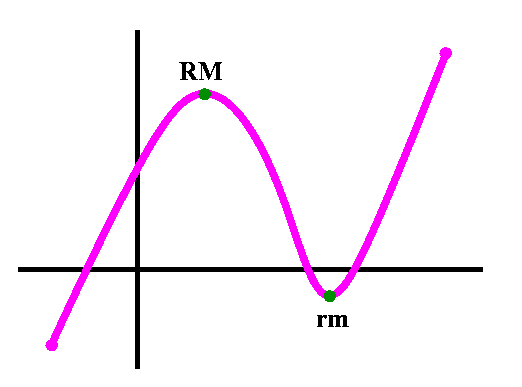
The top of the graph is a Relative Max and the
bottom is a Relative Min. The endpoints are not eligible
to be relative extrema because the function is not defined in an
interval containing either of them in its inside.
|

There is no Relative Max (again each endpoint is not
eligible since the function is not defined in an interval containing
that point). There's a Relative Min where indicated, because
nearby points (on both sides) have larger function values.
|
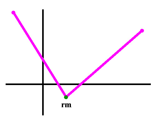
The bottom of the graph is a Relative Min. There are no points
representing a Relative Max.
|
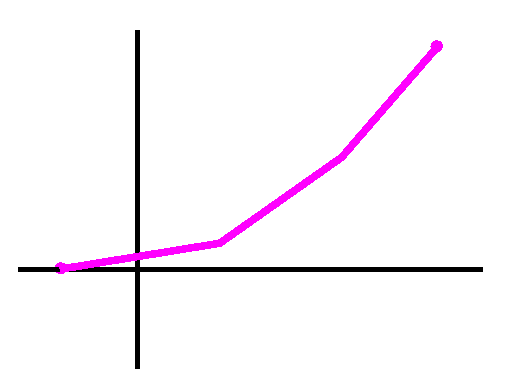
There are no Relative Max and no Relative
Min in this picture. The highest and lowest points are on the ends
which aren't eligible.
|
Definition #3
Suppose the function f(x) is defined at c. Then f(x) has a critical number at c if
- either f´(c)=0
- or f(x) is not differentiable at c.
Then (c,f(c)) is called a critical point of f(x).
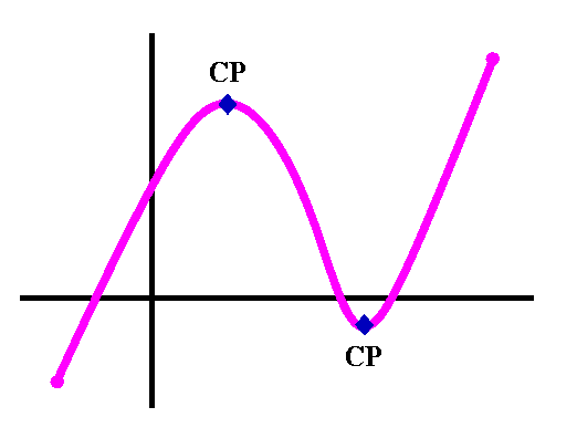
The tangent line is horizontal at the top and the
bottom. At these points, f´(c)=0, so these points are
Critical Points.
|
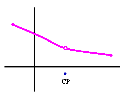
The function is not continuous at a point so the derivative doesn't
exist there. But points where the derivative doesn't exist are still
Critical Points.
|
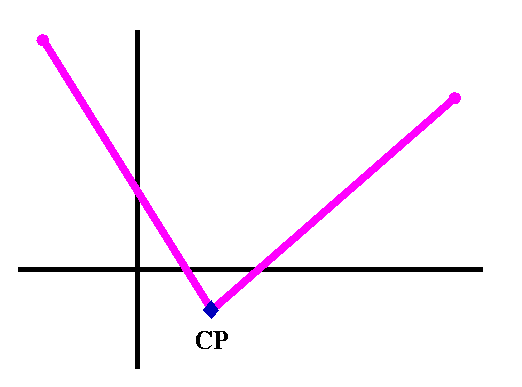
The function is not differentiable at the corner since the left- and
right-hand limits defining the derivative don't agree there. The
corner is a Critical Point.
|
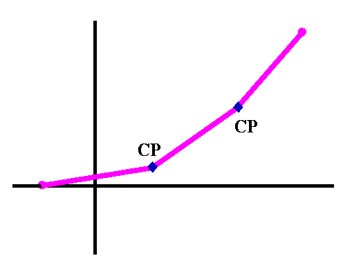
There are two points where the derivative doesn't exist and these are
Critical Points.
|
An important inference
These examples and the others I displayed were supposed to help people
to believe that if f´(c) exists and wasn't 0, then nearby values
of f(x) were higher or lower, so that c was not a relative
extremum. The following statement (the "inference" I mentioned) would
be true:
|
Relative extrema occur only at critical points.
|
Here is an "if ... then" statement of the same inference:
|
If c is a relative max or min, then (c,f(c)) is a critical point.
|
Vocabulary
One definition of inference is "the forming of a conclusion
from premisses." Of course, a definition of premiss is "a
previous statement from which another is inferred." Does this help?
A verification of what happens at relative maxes
Suppose f(x) has a relative maximum at c. Also let me suppose that
f(x) is differentiable at c. Then look at the quotient:
[f(c+h)-f(c)]/h. I will look at two cases:
h is positive: the secant line is to the right of (c,f(c)
Here since f(c) is bigger than f(c+h), I know that the top of the
quotient is negative. But the bottom is positive. Therefore the
quotient is negative divided by positive, and so it is
negative. Secant lines from the right all have negative slopes.
|
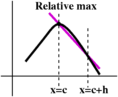
|
h is negative: the secant line is to the left of (c,f(c)
Still f(c) is bigger than f(c+h), so the top of the quotient is
negative. But the bottom is now negative. Therefore the quotient is
negative divided by negative, and so it is positive. Secant lines from
the left all have positive slopes.
|
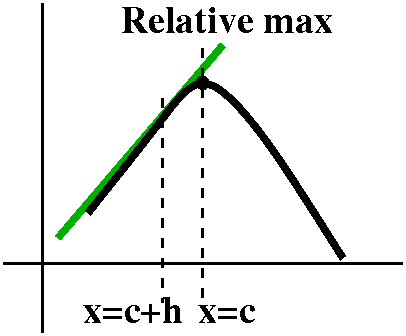
|
Now suppose f(x) has a relative maximum at x=c. If f(x) is
differentiable at x=c, then the previous remarks show that the
derivative is the limit from the left of positive slopes and is also
the limit from the right of negative slopes. The two-sided limit can
exist only when it is 0, so f´(c)=0. Therefore we verified that
at a relative max, then either f´(c) does not exist or if f´(c)
does exist, then it must be 0.
The result for relative mins is proved in the same way.
Some algebraic examples of critical points
| The functions | Sketch of the graphs
(A
machine helped me with these.) |
|---|
|
#1
What are the critical numbers of
f(x)=(1/3)x3+(1/2)x2-6x?
So f´(x)=x2+x-6=(x+3)(x-2), and this is 0 when x=-3 or
x=2.
The critical numbers are c=-3 and c=2.
|
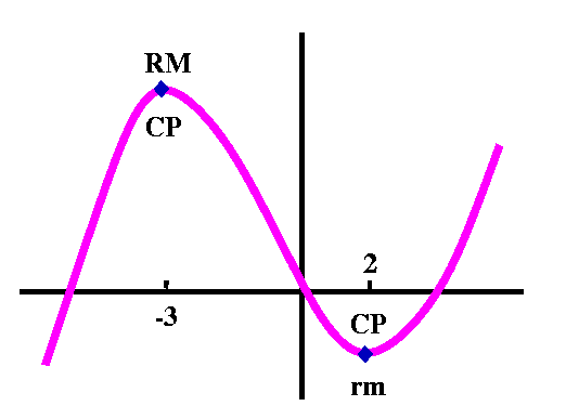
|
|
#2 What are the critical numbers of
f(x)=x2e-3x?
Here
f´(x)=2xe-3x+x2(-3e-3x)=(2x-3x2)e-3x. Since
the exponential function is never 0, the derivative is 0 only when
2x-3x2=0, which is when x(2-3x)=0.
The critical numbers are
c=0 and c=2/3.
|
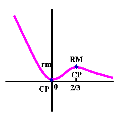
|
|
#3 What are the critical numbers of
f(x)=x2/3(x-2)?
Now f´(x)=(2/3)x-1/3(x-2)+x2/3(1). Stay alert! Algebra coming. I will rewrite this as
a product, because when I write it as a product,
the result will be equal to zero exactly when either of the factors is
0.
I get f´(x)=x-1/3[(2/3)(x-2)+x]. Now
when x=0, the first factor, x-1/3, doesn't make any sense
because the negative exponent means that we would be dividing by 0. So
0 is a critical number of f(x), because the derivative is not defined
at 0. The second factor, (2/3)(x-2)+x, is equal to 0 when
(2/3)(x-2)+x=0, which happens when 2(x-2)+3x=0 or when 5x=4 or when
x=2/5. So 4/5 is also a critical number of this function.
The critical numbers are
c=0 and c=4/5.
|
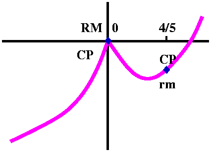
|
In general, if I give you a "random" function, finding out where the
function is "highest" or "lowest" might be very difficult. But the
inference allows one to throw out points which can't be highest or
lowest. But here are two more definitions:
Definition #4
A function f(x) has an absolute maximum at c in an interval if
f(c)>=f(x) for all x in that interval.
Definition #5
A function f(x) has an absolute minimum at c in an interval if
f(c)<=f(x) for all x in that interval.
If you look at the examples and at the inference above then you
should believe that
Absolute maxes or mins of a function on an interval
can occur only at critical
numbers or endpoints.
|
The geometric idea is that if a function has a non-zero derivative at
a number, then the function's graph and its tangent line stick close
together, so such a point can't be a relative max or min: the
tilted tangent line forces the function to be higher on one side of
the number and lower on the other side. So search for relative
{max|min}'s where the derivative doesn't exist (a "corner") or where
the derivative is 0 (a "flat point").
Two dots on the graph ...
I drew coordinate axes with two big dots on the x-axis and urged
students to come up and draw a graph going through the two dots. I got
several graphs similar to what is displayed.

I observed that in each case there were points on the graph where the
tangent line was horitizontal. Below are the graphs with those points
and parts of the tangent lines displayed. Only, I was rude and the first graph below, with a bad
point. People really like to draw s-m-o-o-t-h curves.

The logic of the situation is this: if the function is positive
between the two points, then it has a positive relative max inside the
interval. That must be a critical point (horizontal tangent or not
differentiable). If the function is negative, then ... the same
situation below the x-axis. (Hey, yeah, if the function is never
positive and never negative, then it has lots of horizontal tangents,
because the graph is itself a horizontal line.)
Several versions of Rolle's Theorem
Here's an informal description: if there are two
dots on the x-axis which are part of the graph of a function, then
either the function has a bad place in between or has a flat place
somewhere in between. Since "bad" and "flat" are not usually
considered precise and suitable words in Math 135 (and there are other
implicit assumptions such as continuity), let's rephrase this
statement. Also, the way the result is applied usually assumes that
the function is differentiable everywhere, so the "bad" alternative
vanishes.
Rolle's Theorem (official version)
Suppose f(x) is a
differentiable function, and f(a)=0 and f(b)=0.
Then there is at least
one number c between a and b so that f´(c)=0.
|
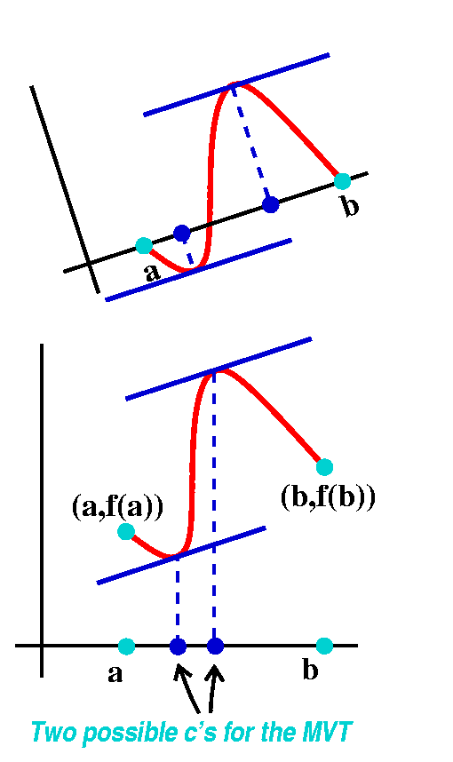
Tilting Rolle's Theorem
People rarely use Rolle's Theorem directly. The hypotheses are rather
strict. Usually the result is tilted, as in the accompanying
picture. But the picture is not labeled conventionally, so the second
picture is what you see in calculus books most of the time. There are
some lines in the second picture which are parallel. The line
connecting the points (a,f(a)) and (b,f(b)) has slope
[f(b)-f(a)]/[b-a] (difference in second coordinates divided by the
difference in the first coordinates). The other lines have slope given
by the derivative of f(x). So you get the statement of the Mean Value
Theorem, which is below.
The Mean Value Theorem (MVT)
Suppose f(x) is differentiable. Then there is at least one number c
between a and b so that f´(c)=[f(b)-f(a)]/[b-a].
|
This is one of the major structural (?) results of calculus, and I
will call it MVT. I asserted in class, and really believe,
that everyone uses reasoning with the MVT. Please keep this in mind as
you read these examples.
| 
|
 Francine on the New Jersey Turnpike
Now Francine is driving north on the New Jersey Turnpike, a restricted
entrance highway. Suppose she enters at the first entrance, the
Delaware Memorial Bridge, milepost 1.2. She gets an admission
certificate, with her entrance time (say, 8:00 AM). Later that day (at
9:15 AM) she exits at New Brunswick, exit 9, milepost 83.3. Let's
think. Let f(t) be Francine's position on the NJ Turnpike at time
t. Here I'll measure t in hours starting at 8:00 AM. I'll measure f(t)
in miles from the southern end of the turnpike (mile 0). So f(0)=1.2
and f(1.25)=83.3. According to the MVT, there is at least one time, c,
between 8 AM and 9:15 AM, at which f´(c), the instantaneous
velocity of Francine (and her car!), is equal to
[f(1.25)-f(0)]/[1.25-0]=(83.3-1.2)/1.25=65.68 (miles per
hour). Therefore Francine automatically gets a ticket for speeding
since tthe
NJ Turnpike authority declares:
|
Unless otherwise posted (due to inclement weather, construction, etc),
the Turnpike speed limits are as follows: The speed limit is 65 MPH
from Mile Marker 1.0 to Mile Marker 97.2.
|
This should a realistic way of enhancing revenue on the Turnpike (for
the state, of course!) and the computational load is not great.
Tuesday, July 11
I went backwards and discussed exponential stuff more, because I don't
think I did a good enough job in class last time. The diary notes are
fine, but the classroom performance wasn't: apologies.
We first looked at interest, in the financial sense: simple interest,
compound interest, and compound interest with an annual rate and
different time periods for compounding. By the way, in reading
about this on the web today, I learned the word
anatocism, which is a legal word for compound interest. The
word was used with this meaning, according to the Oxford English
Dictionary, in 1656.
We went over the discussion I wrote about in the previous
diary entry. I hope that the discussion verified the following
formula, which is frequently used:
Suppose we borrow a principal sum of money, P, for t years, at an
annual rate of interest r, which is compounded m times each year. Then
the amount owed is
(1+{r/m})mt
and we can rewrite this as
((1+{r/m})1/{r/m})rt
using the rule (AB)C=ABC. The reason for doing this
rewrite is so that we can see what happens as m gets larger and
larger. Then {r/m}-->0. And we have the following:
(
(1+LITTLE)1/LITTLE
)rt. We can possibly recognize
(1+LITTLE)1/LITTLE as an approximation to e (see the
discussion during the previous lecture), and this
approximation gets better and better as LITTLE-->0. So
the limit is Pert. (The variables here, spelling out the word
"pert" actually are used in a great many applications.)
Some differentiations
We differentiated a bunch of examples involving the exponential
function. I remarked that some texts favored exp(x) instead of
ex, because the typography (type setting) is easier without
superscripts! Then we could write exp´(x)=exp(x). We could also
call exp(x) the function, "e-to-the". Then it is easier to think that
the derivative of e-to-the is e-to-the. And a composition such as
ecos(x) can be thought of, in f(g(x)) fashion, as taking x
and changing it into cosine of x, and then changing that into e-to-the
cosine of x. So the derivative, f´(g(x))g´(x), would be
e-to-the applied to cosine of x
multiplied by the derivative of the "inside" function, cos(x),
which is -sin(x). So the derivative of ecos(x) is
ecos(x)(-sin(x)).
And then we turned towards logarithms.
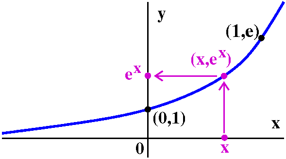 exp
exp
To the right is a graph of the exponential function,
y=ex. I know some things about ex. Of course,
(ex)´=ex, because we chose e to work
that way. But I also know that the domain of ex is
all real numbers, and the range of ex is all positive
numbers. Look at the graph. I could take a number on the horizontal
axis, x, and push it up until it "encounters" (hits) the graph. The
coordinates of that point would be (x,ex). Then if I push
to the vertical axis, the result would be ex there.
Why not relabel? Take some point, w, on the vertical axis, and define
a new function of w by pushing it to the right until it hits the
curve, and then down. The number on the horizontal axis will be called
the natural log of w, usually written ln(w).
ln
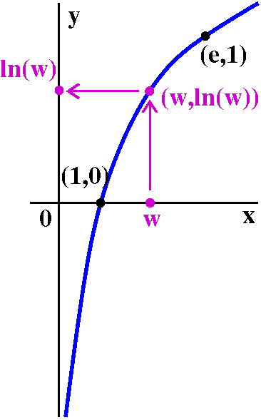 The standard way to think about this is to pick up the graph of
y=exp(x) and flip it over the "main diagonal line" (y=x). This has the
effect of interchanging the horizontal and vertical
axes. There's also an algebraic interchange: the first and second
coordinates are swapped.
The domain of ln is all positive real numbers, and the range of ln is
all real numbers. There are algebraic log properties which are the
reflection (!) or counterparts of the exponential properties:
| Logarithmic rules |
|---|
ln(AB)=ln(A)+ln(B)
ln(A/B)=ln(A)-ln(B)
ln(1/B)=-ln(B)
ln(AB)=Bln(A)
ln(1)=0
|
The "applications" of logarithms in common use which might be
encountered outside of a math course include pH (which is minus the
log base 10 of the hydrogen ... who let that mole in here?) and allied
chemical concepts, the Richter scale (this is a logarithmic scale
which describes the strength of earthquakes), and decibels, a
logarithmic scale for the loudness of sound. But all of this might be
interesting but for us it turns out that there's an essential use for
logarithms in calculus. So let's see it.
We will later in the course be interested in reading the Function to
Derivative transition in the reverse order. In fact, then the
right-hand column will be labeled Function and the left-hand column
will be labeled Antiderivative. Well, we tried to compute a few
antiderivatives, and for powers of x a pattern could be seen.
Function
Antiderivative | Derivative
Function |
|---|
| x2 | 2x
|
| {7/2}x | 7x
|
| x6 | 6x5
|
| {-4/5}x6 | -4x5
|
| {1/44}x45 | x44
|
| {1/(-8)}x-8 | x-9
|
| {1/(POWER+1)}xPOWER+1 | xPOWER
|
But of course the last entry in the table will only be valid if POWER is not equal to -1. What if we
wanted a function whose derivative was x-1, that is, 1/x?
Well, consider the following application of the Chain Rule applied to
the composition of the inverse functions exp and ln (we know that exp
undoes ln -- just look at the arrows on the graphs above):
eln(x)=x. Differentiate this equation. The right-hand side
has
derivative 1 certainly, and the left-hand side has derivative
eln(x)ln´(x)=1. But then x·ln´(x)=1 since
eln(x) is x. So, solving for ln´ we get the final
entry (for this course!) in the derivative table:
| Function | Derivative |
|---|
| ln(x)
| 1/x
|
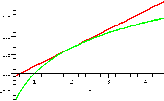 A tangent line
What is an equation for the line tangent to y=ln(x) when x=2?
Well, if we have a point and a slope, then we can find such an
equation. The slope is the derivative of ln(x) when x=2. But that's
1/x when x=2. So the slope is (1/2). What about a point? We need
ln(2), and a calculator supplies us with the (approximate) value
.69315, so the point is (2,.69315). And one possible equation is
y-.69315=(1/2)(x-2).
To the right is a picture of portions of y=ln(x) and
y=(1/2)(x-2)+.69315.
Haven't we seen that number before?
We discussed another homework problem, which was finding the
derivative of
f(x)=[3x-(x4+x)5]3. I asked for
the 100th derivative of this function. This is written
f(100)(x). This is actually easy because I know that
the top degree in this polynomial is 60 (4·5·3) and
differentiation reduces degrees in polynomials by 1. So after 61
differentiations the zero polynomial will be the result.
If you don't believe me, you can check (not easily!) that f(x)=
  60    57     54     51      48      45      42   41      39    38      36     35
-x  -15x  -105x  -455x  -1365x  -3003x  -5005x  +9x  -6435x  +90x  -6435x  +405x

      33      32      30      29      27      26     24      23    22     21
-5005x  +1080x  -3003x  +1890x  -1365x  +2268x  -455x  +1890x  -27x  -105x

      20     19    18     17     16  15    14     13   11     10    7    3
+1080x  -135x  -15x  +405x  -270x  -x  +90x  -270x  +9x  -135x  -27x +27x
Going on ...
Today and tomorrow I will discuss the contents of 6.1 and 6.2 in the
text. This should be the beginning of redeeming my "promise" to show
that the material of this course can be applied to problems and
solutions in areas of student interest. I hope. There will be a bunch
of technical words and phrases, such as
maximum minimum extreme
value relative
maximum relative
minimum critical
point strictly
increasing strictly
decreasing...
Rather than just jumping in and talking so much, I thought I would
rather draw some pictures. Here they are. We'll need to think about
how to
verify these pictures -- or, at least, their qualitative aspects.
| A graph of y=2|x|+4|x-3| |
A graph of y=x3-2x2+x+5 |
|---|
 |
 |
Monday, July 10
We discussed some of the homework
computations.
I distributed copies of the information below. I remarked that the numbers on the
chart were invented, but for the purposes of this class we should
believe they were real. We discussed the chart for a while (an hour is
"a while"!). There's a great deal of information, and I hoped that we
could understand the information.
	                      CHIPCO
                 INVESTMENT DOLLARS & PRODUCTION

Capital Invested    Chips produced       Marginal chips produced
 $ in millions     1,000's of units  1,000's of units per millions $'s

      200               3,000                    .23
      300               3,040                    .28
      400               3,070                    .42
      500               3,100                    .78
      600               3,190                    .31

                         CHIPCO
                    SALES & PROFITS

 Chips marketed      Profit gained           Marginal profit
1,000's of units    $'s in millions  Millions of $'s per 1,000's units


    3,000                1.2                     .03
    3,050                2.8                     .02
    3,100                3.6                     .05
    3,150                4.9                    -.01
    3,200                5.1                     .02
We decided that the pair of numbers 400 and
3,070 referred to the following phenomenon: if the
corporation invests 400 million dollars in capital (building a
factory, furnishing it, hiring and training people, etc.) then
3,070,000 chips can be produced.
Then we tried to understand the third column. The word "marginal" is
used in a fairly technical sense, although the use is common in
economics. In the first table above, it refers to the approximate
amount that chip production would increase per each million dollars of
increase in capital investment. Therefore, for example, if $302
million were invested, then (according to this model) chip production
would be 3,040,000 (chip production at the $300 million level)
plus .28(2)(1,000) chips. The 2 comes from the
additional millions of dollars of capital. The 1,000 comes from the
units used for chip production. The .28 is this "marginal"
quantity. In the first table, the marginal quantity is therefore the
approximate amount  P/
P/ C, relating the change
in chip production to the change in capital investment. It is
sort of a slope, or, more likely, sort of a derivative: indeed, the
use of "marginal" in economics usually means a derivative. In this
model, if $297 million were invested, the approximate expected chip
production would be 3,040,000 (again, chip production at the $300
million level) plus .28(-3)(1,000). The novelty
here is the use of the minus sign, since the capital investment is
decreasing rather than increasing.
The marginal production may vary because at different levels, maybe
different new machines have to be purchased, or different types of
employees need to be hired and trained, etc. Things aren't simple. I
hope that students can recognize the third column of the table was
actually a list of values of the derivative of production with respect
to the "independent variable", capital invested. The textbook
economics definition is the amount of production increase if there is
1 more increase of capital (all using the correct units for this
situation).
The second table describes a similar phenomenon, here connecting the
chip amount, C, with the profit derived from these marketing and sale
of these chips. For example, the profit derived from the sale of
3,000,000 chips (the first line of the second table) is $1.2
million. If we now look at the third column, the model predicts a
marginal profit of .03 (in the given units). Using this, if 3,010,000
chips are marketed (that's 10 more 1,000 units of chips) the
additional profit would be .03(10) million dollars, or $300,000. And
if only 2,970,000 chips were marketed, then the profit would be 1.2
million+(.03)(-30)(1,000)million. (I think I got all the units
correct.) The third column gives  P/
P/ C for various
amounts of chip marketing: the change in profits compared to the
change in chips marketed. One of the numbers in the third column is
negative: the -.01 at the 3,150 level. Is this realistic? Here is what
could happen with a much more modest "business". I could deliver
newspapers every morning. Say that I have 100 customers, located on
five consecutive blocks of one street. It is easy and efficient for
newspaper delivery: the costs are low. What if I get 1 additional
customer? Well, if the customer lives "across town", with a half-hour
of driving needed, taking on this additional business will actually
probably cost money. There may be reasons that the business is
desired, but on a direct basis the incremental profit is negative
rather than positive.
Of course the validity of such models can certainly be criticized, but
I really wanted to show you these tables to explain what's in the next
paragraph.
The two tables linked together describe a complicated
phenomenon. First we "input" capital, M (M is for money), which
produces C, a certain number of chips. Then the chips are marketed
(and sold, hopefully!) to obtain a certain amount of profit, P. Here
we have a composition of functions. For example, suppose we were asked
how much profit there is if we put in M=500 million dollars. From the
first table we read off C=3,100,000 chips, and from the second table
we can then see that P will be 3.6 million dollars.
I hoped that this was all fairly clear. Now I asked what I thought was
a difficult question. Suppose we increase M from 500 million dollars
to, say, 503 million dollars. What will the model predict the likely
profit will be? We can trace this if we are sufficiently alert. The
first marginal quantity we need to consider is  C/
C/ M. For M=500 million dollars,
this is .78. So the new chip production is old chip production +
increase in chip production, and this will be
3,100,000+(.78)(3)(1,000). Now let us consider the chip/profit
table. With C=3,100,000, we see that profit is supposed to be 3.6
million. But we are changing C by adding on the (relatively small)
amount of .78(3)(1,000). The relevant marginal quantity here is
  P/
P/ C, on the row where C is
3,100(,000). The marginal amount here is .05, so that the new profit
will be the old profit (3.6 million) plus (.05)(.78)(3)(1,000) million
dollars. The 3 comes from perturbing the capital investment. The 1,000
comes from my weird units. The really interesting stuff is (.05)(.78):
indeed, this represents the marginal profit as capital invested
changes, when the capital investment is 500 million
dollars. Symbolically, the multiplication might make sense written
this way:
 P
P  P
P  C
--- = --- ---
 M
M  C
C  M
M
So the  C's just seem to
cancel out. This multiplication of rates is typical of what
happens when a composition changes. This is more complicated than
just multiplying fractions, since the fractions (the marginal stuff,
the derivatives) need to be "evaluated" on the appropriate rows of the
tables. But the key idea is that the rates multiply, but you need to
evaluate the rates at the correct inputs.
Further comments
The method used can certainly be criticized. For example, the marginal
cost of chip production at the level M=200 is .23 and at M=300 it is
.28. What do we know about the marginal cost at, say, 350? In my
examples, I was very careful to consider only changes which were quite
small compared to the original quantity. I would not want to use these
ideas far away from the known data. I would need to rethink my
model.
It is easy to get interesting compositions and rates of change in
biology. The transmission of influenza through humans and other
species (birds, pigs) provides very interesting examples, although I
think the biology is more difficult to explain than the economics
behind the tables above.
And about the environment ...
Here's a quote from a Stanford web page, and they should know, since
"Silicon Valley" is immediately to the south:
It takes roughly 10 gallons of water to make a single computer chip.
That may not sound like much, but multiply it by the millions of chips
made each year, and the result is a large and rapidly growing demand
for water. A typical semiconductor factory makes about 2 million
integrated circuits per month and gulps about 20 million gallons of
water, which ultimately must be disposed of as waste. Chips makers
also use large amounts of energy and many toxic chemicals, all of
which can harm the environment.
What's going on?
I tried to present heuristic evidence that
would allow us to believe the chain rule.
/heuristic/ adj.
1. allowing or assisting to discover.
2. [Computing] proceeding to a solution by trial and error.
The Chain Rule Suppose that f and g are differentiable
functions. Then F(x)=f(g(x)) is differentiable, and
F´(x)=f´(g(x))·g´(x). Or:
| Function | Derivative |
|---|
| f(g(x))
| f´(g(x))·g´(x)
|
Here F(x) is the composition of the functions f and g. The tables
above indicate that chip production was a function of capital
investment, and then that profit was a function of the chips
marketed, so that profit as a function of capital investment was a
composition of the two functions.
Examples
My first
example was something like this (about as simple as I could
imagine):
If F(x)=(x2+7)300, what will F´(x) be? Success
here probably will result from recognizing that the chain rule
applies.
If F(x)=f(g(x)), then g(x) is x2+7 so g´(x)=2x, and f(x) is
x300 so f´(x)=300x299. Thus
F´(x)=f´(g(x))g´(x)=f´(x2+7)(2x)=300(x2+7)299(2x).
Whew!
An alternate strategy
You could take the remainder of the summer off and "expand"
(x2+7)300. It is only a polynomial of degree
600. And then it will be easy to differentiate this as a sum of
constants multiplying monomials. That's it: report back next fall on
this method. Be sure to get everything correct.
Now for some realistic comments: almost no one ever bothers to
write all of the intermediate steps. That is, in practice
very few f's and g's are actually identified. What happens is that
people see and differentiate the outside most function (f above), put
in the inner function (g) in that derivative, and then multiply by
g'. For example, consider sin(7x3+x2). What is
its derivative? The outside function is sine, whose derivative is
cosine. So I begin by writing and thinking the following:
cos(what's inside)·the
derivative of what's inside.
The result is
cos(7x3+x2)·(7[3x2]+2x).
This expression is
a formula for the derivative of
sin(7x3+x2). Again, I urge you to consider the
significance and necessity (!) of appropriate parentheses in
these expressions. The "argument" of cosine is 7x3+x2
and the cosine expression is then multiplied by the expression
(7[3x2}+2x).
Example
What is the derivative of [sin(x2)]100? I emphasize that this is not
a situation where the 100 and the 2 could be combined.
This is a
triple composition, but don't worry about it: just handle each layer as
you see it.
 The derivative is 100[sin(x2)]99·[-sin(x2)]·2x.
Maybe using the Chain Rule is like peeling an
onion, layer after layer, and each layer when "peeled"
(differentiated?) contains a copy of the contents of its unpeeled
self. Sigh. Sometimes metaphors are really silly. (Why are you crying?
I don't always cry when I peel an onion.)
We did a large number of examples. I tried to mix in the quotient and
product rules, and the derivative of tangent. The formulas were
horrible, ludicrous, silly, etc.
Exponential growth; exponential decay
I "reviewed" this at jet speed. The reason for the quotes is that I
don't think there was much real review -- I just wrote some formulas
on the board.
There are exponential and logarithmic rules which I hope you
know. Although many of them are "wired into" calculators, the need for
people to have some feeling about exponentials is
important in many applications (compound interest is basically
exponentiation, and of course pH calculations are logarithms).
| Exponential rules |
|---|
AB+C=AB·AC
(AB)C=ABC
A0=1
A-B=1/AB
|
Notice that things aren't the same:
For example, the function f(x)=2x is not the same as
g(x)=x2: f(5)=25=32 and
g(5)=52=25.
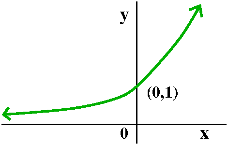 Exponential growth: ax when
a>1
Money This sort of function models compound interest. Suppose
you borrow $10,000 and interest compounds at 5% annually. I'll omit
the $ and the % signs in what follows. Then after one year you owe
10,000+(.05)(10,000). After two years you owe
10,000+(.05)(10,000)+(.05)[$10,000+(.05)(10,000)]. This is
(1+.05)2(10,000). In fact, after t years (t for time) you
owe (1+.05)t(10,000) dollars. This is how the interest
itself makes more interest -- it compounds. Things could also
get more complicated. We could ask what happens if the interest is
entered and charged every halfyear. Then after t years, the amount you
would owe would be (1+{.05/2})2t(10,000) dollars. The .05
is chopped in half because you only get charged 2.5% in half a year,
but the number of compoundings is doubled because the interest
gets credited twice as much. Actually, if the interest, at 5%, is
compounded n times a year, then after t years, the result would be
that you would owe (1+{.05/n})nt(10,000) dollars. Part of
this, (1+{.05/n})n (the t is saved for later) will be
especially interesting. The behavior as n-->infinity gives rise to
what is called continuous compounding.
Bacteria You could imagine the following: bacteria reproduce
(more or less) asexually. So one bacteria (bacterium?) splits into
two, and then each splits some time later, etc. This pattern leads to
exponential growth. So, in the presence of a nice enough environment
(enough food, opportunity to dispose of waste products, etc.) bacteria
reproduce exponentially. The models could be frightening, because
exponential growth, as we shall see, is very rapid. So a slime
mold could easily, within a few days, grow enough to cover the earth
to a depth of 10 feet. Of course this doesn't happen (I think, I
hope!). That's because the validity of the model changes. The
environment won't supply enjoy nutrition, energy, etc. There are more
complex models of bacterial growth (I'll show you the logistic
function later, which is much more realistic). But for simple
situations, bacterial growth is just about exponential.
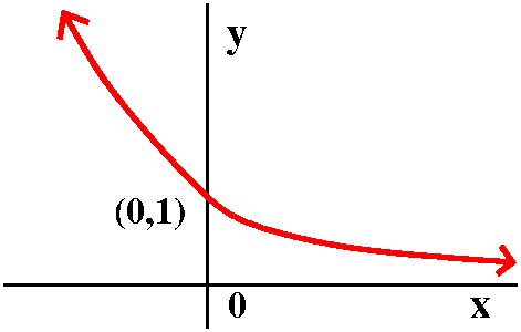 Exponential decay: ax when
0<a<1
Radioactivity Here the model is a chunk of "stuff" made up of
insane atoms. Each atom flips an unfair coin independently, and when
the coin shows tails, does nothing. If the coin shows heads, the atom
changes into another type of atom, usually emitting some sort of
radiation. For example, we could imagine the atoms having one chance
in 100 of changing each second. If we started with 10,000 atoms, then
after 1 second we'd expect (.01)10,000 atoms to flip or change and
we'd expect to have (1-.01)(10,000)=.99(10,000) atoms left of the
original kind. In 2 seconds, we should have
(1-.01)2(10,000) atoms of the original kind. In t seconds,
we would likely have
(1-.01)t(10,000)=(.99)t(10,000) atoms
remaining. Here a=.99, a number between 0 and 1. The horror with
which the world views radioactive decay is that the "transitions" from
one type of atom to another can be accompanied, as mentioned above, by
the emission of harmful radiation. And this can go on for quite a
while.
Mortgage amortization This is like compound interest in
reverse. Here money is borrowed in a big chunk (the principal amount),
and then payback occurs in payments composed both of the interest owed
and part of the principal. For example, below are shown the first five
payments of a $100,000 load at 10% with 12 payments a year and the
last five payments. Notice how much interest is paid cumulatively.
Payment  Principal   Interest   Principal  Cumulative Principal
number    payment     payment    repaid     interest   balance

  1	  488.18      833.33 	 488.18     833.33     99511.82
  2	  492.24      829.27   	 980.42    1662.60     99019.58
  3	  496.35      825.16 	1476.77    2487.76     98523.23
  4	  500.48      821.03 	1977.25    3308.79     98022.75
  5	  504.65      816.86 	2481.90    4125.65     97518.10
                     10 years go by ...
116	 1267.80       53.71   94822.90    58472.26 	5177.10
117	 1278.37       43.14   96101.27    58515.40 	3898.73
118	 1289.02       32.49   97390.29    58547.89 	2609.71
119	 1299.76       21.75   98690.05    58569.64 	1309.95
120	*1309.95       10.92  100000.00    58580.56 	-0.00
*The final payment has been adjusted to account for payments
having been rounded to the nearest cent.
I got these numbers from a web page of
Bret Whissel. Links on that page (especially the link labeled, "More
about this calculator") describe the math used. The key is essentially
a decreasing exponential function but adjustments need to be made to
be sure that the payments actually all work out neatly.
Rates of change of exponential functions
Well, if f(x)=ax, I'd like to get the derivative of
f(x). So I need to look at limh-->0{f(x+h)-f(x)}/h. So:
      ax+h-ax          axah-ax         ax(ah-1)            ah-1
 lim --------- =  lim -------- =  lim --------- = ax lim ------
h-->0    h       h-->0    h      h-->0    h         h-->0  h
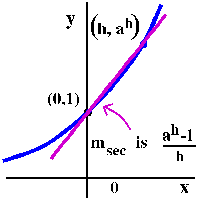 I can't just plug in h=0 because otherwise I'll be dividing by 0. Then
I try some algebraic manipulations to perhaps reveal what is really
going on. The only thing I get is a common factor of ax
which, since there's no h in it, I can bring "out" of the limit. I
need to look at the limit as h-->0 of {ah-1}/h.
The slope of a secant line
Look at y=ax. When x=0, then y=a0=1, so (0,1) is
on the curve. The situation when h is a small positive number is shown
in the picture. Then (h,ah) is on the curve
y=ax, and the slope of the secant line connecting these
two points is [ah-1]/[h-0]={ah-1}/h.
The second page of the Chipco
information contained pictures like those below. The limit as h-->0 of
{ah-1}/h is rather subtle, and I first looked at it with
a=2.
| Graphs of y=2x and y=.69315x+1 |
 |
 |

|
| On the interval -2≤x≤2 |
On the interval -.2≤x≤.2 |
On the interval -.02≤x≤.02 |
|---|
I will explain later where I got the weird number, .69315. But the
"zooms" of the images seem to show that 2x is
differentiable, and that its derivative at the origin, its local
slope, is .69315 because the straight line and the curve just
about totally overlay one another in the third graph.
| Graphs of y=3x and y=1.09861x+1 |
 |
 |

|
| On the interval -2≤x≤2 |
On the interval -.2≤x≤.2 |
On the interval -.02≤x≤.02 |
|---|
Again, I will explain later where I got this weird number, 1.09861. These
"zooms" of the images seem to show that 3x is
differentiable, and that its derivative at the origin, its local
slope, is 1.09861, again because the line and the curve are nearly the
same in the third graph.
Now I don't want to deal with weird numbers like 1.09861 and .69315
because I am lazy. 2x is too shallow and 3x is
too steep. Maybe there is a MYSTERY number,
M, so that Mx has exactly
slope 1 at x=0. That would be nice (and choosing M
would be very analogous to using radians instead of degrees: the
derivative would be so much easier. Well look at this:
| Graphs of y=Mx and y=1x+1 |
 |
 |

|
| On the interval -2≤x≤2 |
On the interval -.2≤x≤.2 |
On the interval -.02≤x≤.02 |
|---|
Discussion of the hypothetical number M
What can I tell you about M? Well, if h is very small,
(Mh-1)/h is approximately 1. What's a small
h? We could try maybe h=1/100.
Since
(M1/100-1)/{1/100} is approximately 1 we
could multiply by 1/100 and see that
(M1/100-1) is approximately 1/100.
Now add 1 to both sides and see that
M1/100 is approximately 1+{1/100}.
If we
took the 100th power (raised things to the 100) then the
1/100 and 100 in the exponent of M cancel (repeated
exponentiations multiply) so that
M is about
(1+{1/100})100.
This is, by the way, 2.704813829. Well, you can see it in the
accompanying table which was handed out, a great souvenir, in class. Give one
to your friends.
This whole chain of ideas was first discovered several hundred years ago by
Euler. In honor of Euler, and also to remember the word "exponential",
the mystery number is called "e", and the attached exponential
function is usually called the exponential function.
The computational strategy shown here for e can be proved to
converge but it does converge rather slowly. For example,
when n=1,000,000, the approximation is 2.718280469 and e is actually
2.718281828459. So even the millionth power is only correct to 4
decimal places. There are faster strategies.
Here is
just about the last derivative formula (except we'll also get a
formula for logs later):
This function is its own derivative because that's how we chose e! The
limit should be 1 for limh-->0{eh-1}/h. I hope
you also see a coincidence coming from the discussion of compound
interest. If you compound a 5% loan n times each year for t years, a
formula for the amount is
(1+{.05/n})nt(10,000). But this turns out, as
n-->infinity, to be the same as (10,000)e.05t. Hey, isn't
that cool!
|
| n | (1+{1/n})n |
|---|
| 1 | 2.000000000 |
| 2 | 2.250000000 |
| 3 | 2.370370369 |
| 4 | 2.441406250 |
| 5 | 2.488320000 |
| 6 | 2.521626376 |
| 7 | 2.546499699 |
| 8 | 2.565784514 |
| 9 | 2.581174789 |
| 10 | 2.593742460 |
| 20 | 2.653297705 |
| 30 | 2.674318750 |
| 40 | 2.685063838 |
| 50 | 2.691588029 |
| 60 | 2.695970192 |
| 70 | 2.699116318 |
| 80 | 2.701484941 |
| 90 | 2.703332434 |
| 100 | 2.704813829 |
| 200 | 2.711517123 |
| 300 | 2.713764888 |
| 400 | 2.714891744 |
| 500 | 2.715568521 |
| 600 | 2.716020591 |
| 700 | 2.716341924 |
| 800 | 2.716584847 |
| 900 | 2.716772937 |
| 1,000 | 2.716923932 |
| 10,000 | 2.718145926 |
| 100,000 | 2.718268237 |
| 1,000,000 | 2.718280469 |
|
Maintained by
greenfie@math.rutgers.edu and last modified 7/10/2006.
 Example 0:
f(x)=(1/4)x4+(1/3)x3-x2+1
 Example 1: f(x)=e-x2
 Example 2: f(x)=(6+7e5x)/(3+e5x)
 Example 3: f(x)=(5x2-3)/(x2+2)
 Example 4: f(x)=x1/3(x-2)
 Example 5: f(x)=x2/e5x
 The inflation rate is, essentially, already C´(t). So C´(t)
is negative and decreasing (remember to use both magnitude and sign
to think about this). Therefore C´´(t)<0. As we move
from left to right (time increases) the slope of C(t) is decreasing.
 Again, the inflation rate is, essentially, already C´(t). So C´(t)
is positive and decreasing (remember to use both magnitude and sign
to think about this). Therefore C´´(t)<0. As we move
from left to right (time increases) the slope of C(t) is decreasing
although it is certainly always positive.
 The inflation rate is, essentially, already C´(t). So C´(t)
is positive and increasing: this is a real data set (as far as I know)
so it isn't "perfect" -- it is {mostly|sort of} increasing!
Therefore C´´(t)>0. As we move
from left to right (time increases) the slope of C(t) is increasing.


 f(x)=x3-3x


 What about 5sin(3x)? Here the 5 just gets carried along, but no higher
derivative is going to be the zero function. Each derivative will
"spit out" (due to the Chain Rule) a 3 to multiply the result. But
what about the other parts of the function? Well sine and cosine do a
dance (?!) when differentiated. The dance steps are pictured to the
right. It is sort of a waltz (forget about the 3x inside for a second,
please). Every fourth step brings us back to where we were. So if we
wanted the 78th derivative of sine, we would divide 78 by
4. This would be 19: but not exactly -- there would a be a remainder
of 2. This means that the 78th derivative waltzes around
this figure 19 times, and then does two more steps, so that the result
would be -sine. Wow (maybe). The result would still have the 5
and 78 of the 3's multiplying and the darn 3x inside the function. But
the waltz makes the computation easy. (I don't want to make things too
darn easy: the derivatives of tan have no simple structure.)


 f(x)=(3x+5)/(x2+1)
 Various computational devices would produce something like what is
shown to the right as a graph of f(x)=2|x|+4|x-3|.
 Now let me look at f(x)=x3-2x2+x+5. This is
"easy" (well, maybe). There is one nice algebraic formula defining
f(x). The domain for this polynomial is all real numbers, and
polynomials are continuous and polynomials are differentiable. In
fact, look, f´(x)=3x2-4x+1, so the function sure is
differentiable. I should expect that the graph will have no jumps --
it will have one piece. I should expect that the graph will be a nice,
smooth curve, with a neat tangent line at every point. So far, the
picture to the right should be further evidence of these assertions.


 Francine on the New Jersey Turnpike
 exp
exp The standard way to think about this is to pick up the graph of
y=exp(x) and flip it over the "main diagonal line" (y=x). This has the
effect of interchanging the horizontal and vertical
axes. There's also an algebraic interchange: the first and second
coordinates are swapped.
The domain of ln is all positive real numbers, and the range of ln is
all real numbers. There are algebraic log properties which are the
reflection (!) or counterparts of the exponential properties:
 A tangent line
 The derivative is 100[sin(x2)]99·[-sin(x2)]·2x.
 Exponential growth: ax when
a>1
 Exponential decay: ax when
0<a<1
 I can't just plug in h=0 because otherwise I'll be dividing by 0. Then
I try some algebraic manipulations to perhaps reveal what is really
going on. The only thing I get is a common factor of ax
which, since there's no h in it, I can bring "out" of the limit. I
need to look at the limit as h-->0 of {ah-1}/h.
