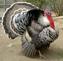To the right is a picture of a male domestic turkey. It has wattles ("a loose fleshy appendage on the head or throat of a turkey or other birds.") which are sort of enlarged jowls ("the external loose skin on the throat or neck when prominent."). Certainly the instructor does not look like a turkey. Domestic turkeys are supposed to be extremely stupid. Wild turkeys, which are much thinner and mostly brown, are quite shy and difficult to observe. They do exist on Busch Campus! Try to find one. (Don't get caught in the Rhus toxicodendron while seeking the Meleagris gallopavo, please.)

Compact ... closed ... bounded ...

Compact implies closed
Suppose p is in X and p is a limit of a sequence of points {k_j} where each of the k_j's is in K. Consider the open set U_n={x in X with d(x,p)>1/n}. Certainly U_n is open and U_n+1 contains U_n. If p is not in K, then {U_n} is an open cover of K, so some finite subcollection of them covers K also. Since the U_n's are nested, then is one U_N which contains K. But if p is a limit of points in K, we have a contradiction: some of the k_j's satisfy d(p,k_j)<1/N. Therefore p must be in K. We have proved that if K is compact, then K is closed in X.

Compact implies bounded
Suppose K is compact. Consider any point p, and look at U_n={x in X with d(x,p)<n}. Of course U_n is contained in U_n+1. Certainly the union of the U_n's contains K (it is all of X!). So (because of finite subcover and the nesting) there is N with K contained in U_N. This means (triangle inequality) that the distance between any two points of K is less than 2N. We have proved that if K is compact, then K is bounded in X.

Extra credit
Which of those proofs is Artinian? Which is Noetherian?

Heine-Borel
The Heine-Borel Theorem declares that if S is a subset of Rⁿ which is closed and bounded, then S is compact. This is not true in all metric spaces.

Example 0
If (X,d) is a metric space, then (X,d/(1+d)) is a metric space with the same topology. In this metric, however, X is bounded. Since X is also closed as a subset of itself, X is closed and bounded. If you believe the converse of "compact implies closed and bounded" you would need to believe that every metric space is compact.
O.k.: this example is silly.

Example 1 Consider the unit disc in R2 (or C!). This is our X, and d will be the usual metric. Look at the subset S of X which is those complex numbers with |z|<1 and Im(z)=0 (the x-axis inside the unit disc). S is not compact. The open cover whose elements are D1-(1/n)(0) (here n is a positive integer) does not have a finite subcover. But S is bounded (hey: the bound is 2, but that's o.k., X is bounded also). And S is a closed subset of X (look at X\S, which is nice and open).
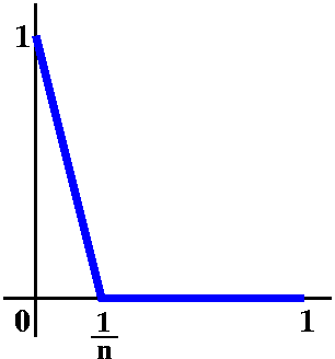
Example 2 Suppose X=C([0,1]), the collection of continuous functions on the unit interval. The distance on X will be the sup norm. That is, if f and g are in X, d(f,g)=supt in [0,1]|f(t)-g(t)|. Since f and g are continuous, the sup is actually achieved: it is a max. Suppose S is the collection of functions whose distance from the 0 function is at most 1. So S={f in C([0,1]) with |f(t)|<=1}. This is the closed unit ball and is certainly closed and bounded. Now look at the functions fn defined piecewise by:    fn(x)=0 if x>1/n; fn(x)=1-nx if x is in [0,1/n]. A picture of a typical fn is shown to the right. Certainly fn is continuous and is in S.
Notice, please, that if x is in [0,1], the function EVx defined by EVx(f)=f(x) (evaluation at x) is continuous on C([0,1]) (evaluation at a point is less than the max of the function!). Suppose the sequence {fn} converges in X. Since EVx(fn)-->0 if x>0 and EV0(fn)=1, the limit would have the value 1 at 0 and be 0 for x>0. This is not a continuous function, so {fn} does not converge in X. Now you use these fn's to create an open cover of S which does not have a finite subcover (this isn't too hard, I think). S is closed and bounded, but not compact.

Of course we are really using here is that C([0,1]) is not locally compact. But that's not very strange. Combinatorists: contemplate a graph with infinite degree at a vertex. If the edges are each like an interval, then that graph will not be locally compact in any natural topology.

What really goes wrong with the example above is that the f_n functions wiggle too much. We will return to consider the issue of wiggling later ("equicontinuity").

Here's another example ...
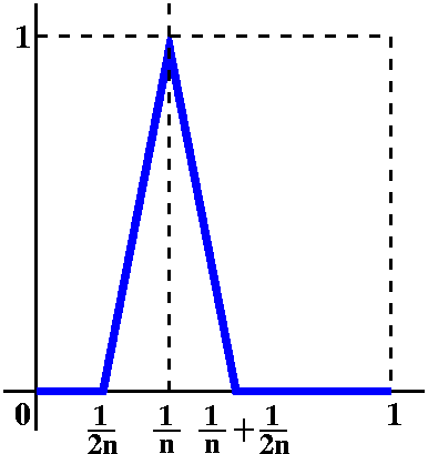This example is maybe a bit more irritating. Define g_n by the following piecewise recipe (really the picture to the right is what I'm thinking of and I only hope that what follows is almost correct):
   g_n(x)=0 if x<1/{2n} or if x>{1/n}+1/{2n};
   g_n(x)=(n+n²)x-(n+1)/2 for x in [1/{2n},1/n];
   g_n(x)=-(n+n²)x-(something) for x in [1/n,(1/n)+(1/{2n})].
Now define h_n=g_(2ⁿ) (that's 2ⁿ in the subscript for the g's). The bumps for the h_n's don't "interfere" with each other. Then:

1. Each h_n is in S, the closed unit ball of X=C([0,1]).
2. The distance between h_n and h_m is 2 if n and m are not equal. They can't converge. This may be very disconcerting to you if you don't believe in "infinite dimensions".
3. Make an open cover of S which doesn't have a finite subcover using these functions: take a ball of radius 1 around each h_n, and then "throw in" X\{all of the h_n's} (the last set is open because the set of h_n's is discrete in X).

Here is the last appearance of the algebra table.

Is this Ring...	C[z]	C{z}	C[[z]]
A UFD?	Yes	?	Yes
A PID?	Yes	Yes	Yes
Noetherian?	Yes	Yes	Yes
Artinian?	No	Yes	?

Mr. Williams and others interacted with the lecturer for this presentation. A key obervation is identifying the units (the invertible elements for multiplication) in the ring of convergent power series. These turn out to be exactly those power series with non-zero constant term. Then ideals etc. can be studied easily.

The lecturer mentioned that the following observations are now almost easy, but proving them from the definitions would be somewhat irritating.

• The inverse of a convergent power series with non-zero constant term is a convergent power series (such a series has sum which is holomorphic, the reciprocal of a non-zero holomorphic function is holomorphic, and that function then is representated by a convergent power series).
• The Cauchy product of convergent power series is a convergent power series (I guess I could do this from the definition, but it still would not be pleasant -- I would prefer to "sidestep" through --> -- holomorphicity).
• The composition of two convergent power series is convergent. Again using the same type of approach as in the previous paragraph yields the result easily. A more direct approach may get involved (for example, combinatorialists should know a bit about Faà di Bruno's formula.

Maximum Modulus Theorem (version 2)

Maximum principle (for harmonic functions)

"Proof"

What! No harmonic conjugate!!

Minimum principle (for harmonic functions)

Hot plates

Uniqueness for the Dirichlet Problem

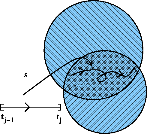
The lecturer mentioned the distinction between "compact" and "closed and bounded" which is discussed further in the special edition above.

The set K_t mentioned in the homework is compact in C for any compact K and non-negative real t, since the mapping Kx[0,t]-->C given by (k,s)-->k+s is continuous and the domain is compact.

We estimated f´ from f using the Cauchy Integral Formula for derivaitives (the same can be done for f⁽ⁿ⁾ by either using the appropriate Cauchy Integral Formula or by "interpolating" more compact sets to get higher derivatives).

The instructor asked if students really believed the result, since, say, sin(nx) on [0,1] is bounded in absolute value by 1 but its derivative wiggles a great deal. How can we "reconcile" this? Of course, the answer is that [0,1] in C is very "thin" and a compact neighborhood of it must stick out into the top and bottom halfplanes. There sin(nz) has exponential behavior in both real and imaginary parts, so sin(nz) gets enormous on any such set.

We stated and verified the famous Weierstrass result: if {f_n} is a sequence of holomorphic functions which converge uniformly on compact subsets of an open set U, then so do the sequence of derivatives, {f_n´}. Therefore the u.c.c. limit of such functions is itself holomorphic, and, in fact, all derivatives converge to the appropriate derivative of the limit.

This means that "construction" of a holomorphic function can be much easier in some technical sense than, say, construction of a C function was for Borel's Theorem.

Let R_N be the N^th roots of unity, and let NR_N be that set multiplied by N. If R is the union of NR_N for N>1, we "constructed" an explicit function which was holomorphic on all of C\R. This was very easy using the Weierstrass Theorem.

Mr. Williams suggested a few entries in the algebra table.

Is this Ring...	C[z]	C{z}	C[[z]]
A UFD?	Yes	?	Yes
A PID?	Yes	?	Yes
Noetherian?	Yes	?	Yes
Artinian?	No	?	?

We began by recalling a theorem from last time with a picture in mind.

Theorem If f is holomorphic in an open connected set U, and if f=0 (f equals the zero function!) in some disc contained in U , then f=0 in U .

Corollary If f and g are holomorphic in U, and if f=g on some disc contained in U, then f=g on U.

This leads to some questions about the zeros of a holomorphic function: how "often" can a holomorphic function be equal to 0?

First, an entire function is one that is holomorphic on the whole complex plane. For any function f, we define Z(f) to be the set of zeros of f.

1. Question Is there an entire function f with Z(f)=the empty set?
   Answer Sure, take f(z)=e^z.
2. Question Is there an entire f with #Z(f)=1? (Here "#S" is the cardinality of a set S.)
   Answer Take f(z)=z.
3. Question Is there an entire f with #Z(f)=2? Answer Take f(z)=z(z-1). And in general, taking f(z)=(z-1)(z-2)···(z-n) will give an entire f with #Z(f)=n.
4. Question Is there and entire f with #Z(f)=?
   Answer Well, f(z)=0. But if we add that f is NOT the zero function, then we can take f(z)=z(e^z-1), since Z(f)={2n(Pi)i | n is an integer}.
   
5. Question Is there an f holomorphic in D₁(0) with #Z(f)=?
   Answer Take f(z)=e^(i/(1-z)). Then for z=1-1/(2nPi), z is in the disc and f(z)=0.
6. Question How about Z(f) uncountable? (With f still not the zero function.)
   Answer No! C is sigma compact. This means it is the union of countably many compact subsets. We verify this for C by writing C as the union over all positive integers n of the closure of D_n(0)(the disc of radius n centered at 0). If Z(f) is uncountable then there exists an n>0 so that the numbers of elements of Z(f) in the closure of D_n(0)is infinite (if this is finite for all n then the zero set is the countable union of finite sets and hence countable). Since the closure of D_n(0) is compact, there exists a z^* in D_n(0) which is a limit point of Z(f). Then z_j-->z^* for some distinct z_j in the closure of D_n(o), and f(z^*)=0 since f is continuous. For all e>0, the intersection of D_e(z^*) and Z(f) is infinite. But our local description of f then shows (since f is not N to one for any N) that f must be constnat.

So we can replace the disc hypothesis with the hypothesis that Z(f) has an accumulation point in U in the first theorem and corollary. !!!! excitement!

Basically, if two holomorphic functions agree on a set with an accumulation point in their common (connected) domain then they are equal.

For instance, there is exactly one entire function f such that f(x)=sin(x) for all x in R. More generally, any definition of a holomorphic function which agrees with something on R works.

We also get some nice properties for free. For example, since sin(z) and cos(z) are entire, so are (sin(z))² and (cos(z))², so since (sin(x))²+(cos(x))²=1 in R, (sinz)²+(cosz)²=1 in C. Similarly, sin(A+B)=sin(A)cos(B)+cos(A)sin(B) on all of C follows from the equality of the two functions in R.

Then sin(z)=sin(x+iy)=sin(x)cos(iy)+sin(iy)cos(x). But we already know the Taylor series for cosine on R which must be the power series for cosine on C: cos(iy)=_n=0[(-1)ⁿ(iy)²ⁿ]/(2n)!=_n=0y²ⁿn/(2n)!=cosh(y) and similarly sin(iy)=i sinh(y).

So sin(x+iy)=sin(x)cosh(y)+i sinh(y)cos(x).

What is Z(sine)? Since cosh is never 0, sin(x+iy)=0 implies sin(x)=0, so x=nPi. Then cos(x) is nonzero, so sinh(y)=0, which implies y=0. Thus Z(sine)={nPi | n is an integer}. All of the zeros of the entire function sine are the same as the real zeros of the "calculus function" sine.

Here is a Rutgers qualifying exam problem: Suppose f is holomorphic on a neighborhood of zero, and you know for all integers k that f(1/k)=100i/k⁴. What is f?

Answer The sequence {1/k}_k=1 has an accumulation point in any neighborhood of zero, so since f(z) and 100iz⁴ (A guess! A guess, only!) agree on {1/k}_k=1, f(z) must actually be 100iz⁴.

Philosophy: this sort of says that if a sequential statement can be proved about a holomorphic function (say, for example, by some inductive proof, and if the statement is true on a set with an accumulation point, it is always true. This is almost startling.
So any algebra or simple calculus property which is true on a set with an accumulation point must be true on the whole (connected) open set.

Now we consider the "other case" from last time. If a holomorphic function f is not locally constant, then for all p in U there is a natural number N so that f(z)=a+(k(z))^N where k is holomorphic in some disc of radius e centered at p, k(p)=0 and k´(p)=0.
Notice that in this description, f is a composition of open mappings. These are functions so that the image of any open set is open.

Question Can such a function be a folding of the complex plane?

Answer No, we can't have a holomorphic function which folds C since we can't fit an open set around any image point on the crease. (It is also true that the number of inverse image points around one of the "crease" points varies from 2 to 1 to 0, and this is also impossible.

Open Mapping Theorem Suppose U is an open connected set, and f is a non-constant holomorphic function on U. Then f is an open mapping.

"Proof" We just need to show that open neighborhoods of points in the domain have images which are open. But if f is non-constant, its local description is always like that above, for some positive integer N. The local description takes open sets to open sets, so f is open.

A Calc 3 exam problem Let S=[0,2pi]x[0,2pi], a subset of R². What's the maximum value of f(x,y)=sqrt[(sinx)²(cosh)²+(cosx)²(sinhy)²] on S?
Answer In Calc 3, we would begin by searching for interior critical points. But since we recognize f as |sinz|, there can be no such points. Why? If q were such a point, then f(q)>=f(z) for nearby z. But then sine would map the region near q to those w's with |w|<=q. And f(q) would be on the boundary of D_|f(q)|(0). The points near q would be mapped inside the closure of the disc, and certainly an open neighborhood of q would not be mapped by sine to an open neighborhood of sin(q), which is a contradiction to the Open Mapping Theorem. The max must occur on the boundary (and where is that max? Can you find it?)

Maximum Modulus Theorem (version 0) If f is holomorphic in an open and connectioned set U and f is not constant, then g(z)=|f(z)| has no local maximum.

Remark We can't change "max" to "min". For instance, consider f(z)=z on D₁(0).

Maximum Modulus Theorem (version 1) Suppose U is open and connected, and U closure is compact in C. Suppose f is continuous on U closure and holomorphic on U. Then sup_{z in U closure}|f(z)| exists and equals sup_{z on U}|f(z)|.

Proof |f| attains a maximum since it is continuous on a compact set. One inequality comes for free since U is contained in the closure of U. If f is a constant function, then both sides are the same. By version 0, when f is not constant, the max on U closure cannot be in U, so it is on the boundary.

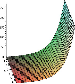
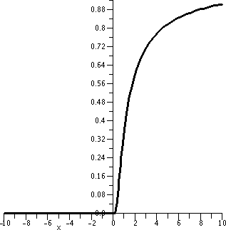
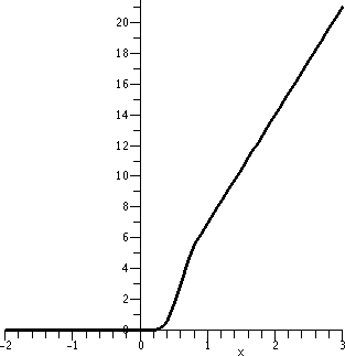
Some computer-drawn pictures
Since we have powerful graphics programs, we should be able to "see" some of these results. Below are two pictures produced by Maple. The picture to the left is the image of |sin(x+i y)| on the rectangle [0,2Pi]x[0,2Pi]. I looked at it and was a bit confused. Certainly what's shown does not seem to have an interior maximum, so that was o.k. But I wanted to see some boundary variation, especially along the boundary part with Im(z)=0. I didn't "see" it. Then I realized: consider the vertical scale. The picture automatically adjusts things (this is Scaling Constrained, the default) so that the image fills the viewing window. The imaginary part involves cosh and sinh. These are basically exponentials, so they grow enormously. For example, the approximate value of |sin(2Pi+2Pi i)| is 267.75. I can't expect to "see" wiggles of 0 to 1 on the border if the vertical scale is several hundred times as high. The exponential growth will be used more in the next lecture. The picture to the right is made with an idea that is not new, but is rather convenient in situations where there's lots of data, and the data may vary in size a great deal. Consider arctan (the usual real calculus function arctan). It is strictly increasing, has domain all of R, and has range (-Pi/2,Pi/2). If we compose data whose size is "unknown" with arctan, then we'll get output which preserves order, but which is restricted in size. (Indeed, this feature is built into Maple itself if you ask for plotting of a function from 0 to , say.) So the picture on the right is arctan(|sin(x+i y)|). Now I can "see" the result of |sin(x)|² when y=0. Since arctan preserves order, there is still no interior local maximum. But there is a penalty (think about this!) in the following: the convexity changes in the y-direction. The left picture has x=constant sections of the graph appearing (correctly) concave up, while the right picture has such sections concave down. Is this correct? (Yes. Why?)

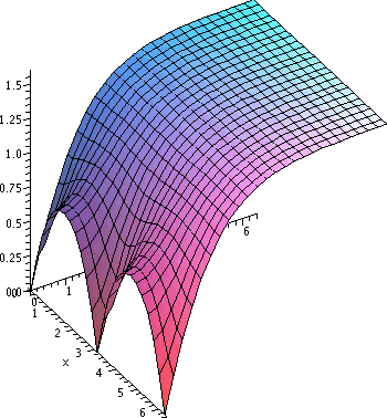|sin(x+i y)|	arctan(|sin(x+i y)|)

During the course of previous lectures, we have encountered the following commutative rings denoted by:

C[z], C{z}, and C[[z]]

which respectively represent the polynomials, convergent power series and formal series in one variable with complex coefficients. Followers of abstract algebra will be quick to remark that there are ring monomorphisms going from left to right, embedding one ring into the next.

The instructor attempted to fill the empty boxes in the following table with "yes" or "no":

Is this Ring...	C[z]	C{z}	C[[z]]
A UFD?	Yes	?	?
A PID?	Yes	?	?
Noetherian?	Yes	?	?
Artinian?	No	?	?

Using sophisticated monte-carlo techniques, the instructor has filled out the first column and requested algebraically inclined students to complete the remainder. We really should know the answers!

We now move on to Goursat's Theorem, which the instructor claimed was remarkable since it made no assumptions regarding the continuity of the derivative, hence "nice to know", but lacking in any practical value whatsoever. (The scribe would be remiss if he failed to point out Avital Oliver's impassioned support of Goursat and the subsequent seal of kosher approval shaped like the Star of David.)

Goursat's Theorem Suppose U is an open subset of C. If for any given function f:U-->C, the limit defining f´(z) exists for all z in U, then f is holomorphic on U.

Proof (A version of the proof that was provided in class is also available in all its glory at planetmath)
By our version of Morera's Theorem, it suffices to prove that the integral of f around any rectangle in U is zero. For contradiction, assume there is a rectangle R so that _Rf(z)dz=A, where A is a nonzero complex number. Then, we subdivide this rectangle into 4 smaller rectangles R₁,...,R₄ so that

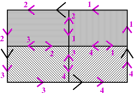
_j=1⁴(_Rjf(z)dz)=A.

This is because the integrals along the "inner edges" cancel. The picture shown is an effort to persuade you that this is correct. The labels are the directions on each boundary segment of the borders of the inner rectangles. Now, we claim that there is at least one j in {1,...,4} so that |_Rj(f dz)|>= |A|/4.

since otherwise the sum of all 4 integrals would have absolute value strictly less than |A|, thus leading to contradiction. We can now reapply our subdivision idea to this R_j. Repeating this process ad infinitum and relabelling the indices allows us to create a strictly decreasing sequence of nested rectangles {R_p,p in N} so that

|_Rpf(z)dz|<= A|/4^p. (Call this (i))

Now we observe that the intersection of all elements of {R_p} must be a unique point by the nested set property,

What is this property? In the following, assume that [Sj}j in N is a nested sequence of subsets of R2. Here nested means Sj+1 is a subset of Sj for all j>=1. Find an example in R2 of a sequence so that the intersection is empty. Find an example in R2 of a sequence whose diameters-->0 so that the intersection is empty. Find an example in R2 of a sequence of open sets so that the intersection is empty. Example (for all three) Sj=(0,1/j)x(0,1/j) in R2, n in N. Certainly diam(Sj)=sqrt(2)/j-->0 as n-->. Find an example in R2 of a sequence of closed sets {Sj} so that the intersection is empty. Example Sj=[j,) (each is a subset of R1 and hence a subset of R2). What is the precise statement of the "nested set property"? What is a (possibly approximate) proof?

so there is a unique z^* sitting in the intersection of all our rectangles. By hypothesis, we know f´(z^*) exists, so for every h in U, we have

f(z^*+h)=f(z^*)+hf´(z^*)+o(|h|)

The first two terms on the right constitute a linear function on U, which is clearly holomorphic, so by Cauchy's theorem the integral of the first two terms around any rectangle in U is zero. So, define

g(z)=f(z)-f(z^*)-(z-z^*)f´(z^*),

and note that if S in U is a rectangle, then

_Sf(z)dz=_Sg(z)dz, (call this (ii))

Now, since g is continuous by and the boundary R_p of R_p is compact for all p, we can set M_p to be the maximum value of g(z) on R_p; if L_p is the length of R_p, we can use the ML estimate to get

|_Rpg(z)dz|<=M_pL_p (call this (iii))

But L_p=L/2^p, where L=R₁, and, since g(z)=o(|z-z^*|), we know that M_p<=(Q_p)2^-p. Further, Q_p-->0 because of the little o part of the differentiation definition. We can now combine (i), (ii) and (iii) and get:

|A|/4^p<=| _Sf(z)dz|<=(Q_p)2^-pL/2^p

Which provides the desired contradiction, since the right side goes to zero faster than the left side for nonzero A. QED

The Goursat Theorem has a proof which is rarely used in other contexts. Let's move on to a point of view and some results which are exploited in many ways. We want to get quite precise local description of f.

Getting a precise local picture of holomorphic functions
Suppose f is holomorphic in some open set containing 0. Then we know that there is R>0 and a sequence of complex numbers {a_n}_n=0 so that f(z)=_n=0a_nzⁿ for all z with |z|<R. Two alternatives occur:

• f is constant in the disc of radius R centered at 0
  So all of the a_n's with n>0 are 0.
• f is not constant in the disc of radius R centered at 0
  There is a positive integer N with a_N not 0 and a_j=0 for 1<=j<N.

f(z)=a₀+z_Ng(z)=a₀+z^Nh(z)(h(z))N=a₀+(zh(z))N.

Define the holomorphic function k by k(z)=zh(z). Then k(0)=0 and, by the Product Rule, k´(0)=a_N, which is not 0.

The easy case
Again we might possibly need to decrease S to some positive number T. But, using the Inverse Function Theorem of "Calculus" in R² (a rather profound theorem!) we can state that k, in the disc of radius T, is a diffeomorphism. That is, k restricted to D_T<0> is a bijection from that disc to an open neighborhood of 0, and both k and its inverse are differentiable. But we know from the homework assignment what the derivative of k is: a directly conformal linear mapping, whose inverse is also directly conformal (this is a linear algebra description of the Cauchy-Riemann equations).

Smooth curves through a point z in the domain with some positive angle are transformed into smooth curves with the same angle through the corresponding image point, k(z). The curves are rotated by arg(k´(z)). The local speed along the curves is multiplied by |k´(z)|. There's just this one rotation and one magnification factor, so locally the picture is easy (!?) to understand.

Power mappings near 0
Let's explore the mapping P defined by z-->z^N for N>1. For N=1, this is covered by the previous paragraph. In a disc of radius T centered at 0, P is "fine" (locally) away from 0, since then P´(z)=Nz^N-1 is not 0. But considered in all of D_T(0), P is N-to-1 except for 0. The inverse of a non-zero w is given explicitly by b(w^1/N) where w^1/N is one N^th root of w (if w=re^iq then one value of w^1/N is r^1/Ne^i/N) and where b is any of the N N^th roots of 1. Remember that the N^th roots of 1 form the vertices of an inscribed regular polygon with one vertex at 0. P's mapping on D_T(0) is an example of what is called a branched covering map.

Covering maps
f:X-->Y is a covering map if for all y in Y, there is a neighborhood N_y of y so that f^-1(N_y) is a disjoint union of neighborhoods N_x for each x in f^-1(y) so that f|_Nx is a homeomorphism from N_x to N_y. Examples of covering maps relevant to this course are z-->z^N on C\{0} (an N-to-1 mapping) and z-->e^z on C (an infinite-to-1 mapping).
It is not necessarily true that all preimages of a point have the same cardinality. For example, consider z-->z² on those z's satisfying 1<|z|<2 with arg(z) between 0 and, say, 3Pi/2. The cardinality of the preimages will be either 1 or 2.

Branching/ramification
People say that the mapping P(z)=z^N ramifies or branches at 0. It is no longer a covering map. The inverse images stick together (?) and become one point. But, except for that failure, P is very nice. The average number (?!) of inverse images is N (well, except for 0, this number is n), and this number is called the degree or the order or the multiplicity ... there are several names. The instructor declared, "This number is used more or less in every area of math I know about."

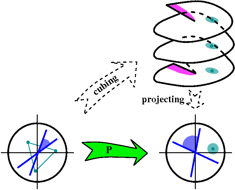
To the right is a diagram which may help you understand the mapping P. This is "specialized" to the case N=3. The topologists tell us that one way to try to comprehend the mapping is to imagine that it is the composition of two mappings. One is "cubing", whose domain is a disc centered at the origin. The range of this mapping, which is 1-1, is a weird topological space. Think of it as D0 and D1 and D2, with an interesting equivalent relation. Here is the equivalence relation: all of the 0's in the discs are equivalent. If (z)j represents the copy of z (for z in the disc) in Dj, then this means that (0)0=(0)1=(0)2 (so all of the origins are the "same" point). What about the other points? Let's pick some random number in [0,2Pi], say v. Then for r>0, I will describe a neighborhoon of (reiv)0: take the z's in an ordinary neighborhood of reiv. If z=aeib, and b>=v, then (z)0 is in the neighborhood of (reiv)0. If z=aeib, and b<v, then (z)2 is in the neighborhood of (reiv)0. Also, (reiv)0=(reiv)2. There is a similar identification with radial edges of the other discs.

What I am attempting to describe is in the complicated picture displayed. The solid black borders of the magenta (?) regions should be "identified". This identification space cannot be constructed in R3 without self-intersection, and what is drawn is a possible representation of it in R3. The mapping which is called "cubing" sends z in the disc to w=z3 in the quotient space, with the specific (w) depending upon whether z is in the first third of the disc (arguments between 0 and 2Pi/3, then j=0) or in the second third of the disc (arguments between 2Pi/3 and 4Pi/3, then j=1) or in the third third of the disc (arguments between 4Pi/3 and 2Pi, then j=2). Writing this is incredibly irritating and hard to understand, so no wonder topologists never really prove [The instructor's legal counsel has redacted the remainder of this sentence.]. Finally, the projecting map just takes (w)j to w. The image of two lines going through the origin becomes two lines going through the origin but the angles involved are multiplied by 3. The inverse image of a point away from the origin is, first, in the covering space, three points. A neighborhood's inverse image is three blobs over the neighborhood. Finally, back in the original disc, the inverse image of a point which is not the origin is three points forming in this case an equilateral triangle (N=3) which has 0 as its center. Wow! The "cubing" part is 1-1, and the "projecting" part is 3-1. The blue lines are just drawn in the domain and range. The cyan points and region are drawn pulling back from the range, into the covering space (for the blob and point) and just the points, together with a possibly useful triangle, in the domain.

The complete local description for non-constant holomorphic functions
So if a holomorphic f is not locally constant, then f must be written as a composition of the mappings z-->k(z) (a [directly] conformal diffeomorphism) and P, which maps z to z^N, an N-to-1 map away from 0, which is conformal except at 0, and which, at 0, multiplies the angle between curves by N, and, finally, the translation, z-->a₀+z. Whew! Well, that is a rather neat qualitative description.

Back to the constant case
Let us "exploit" the first alternative in the local description. What should the "degree" be when f is just a constant term in some power series expansion? People vary with what they say. Sometimes it is asserted this should be 0, and sometimes it is asserted that it should be . Oh well. But being constant spreads throughout a connected open set.

Theorem Suppose U is a connected open set, and suppose that f is holomorphic in U. If there is p in U with the power series expansion of f at p just equal to a constant term, then f is a constant function. Indeed, all of the power series expansions of f are just the constant term.

Proof If n is a positive integer, let C_n be the collection of z's in U with f⁽ⁿ⁾(z)=0. Notice that since f is holomorphic, f must be C, so f⁽ⁿ⁾ is continuous and C_n is a closed set. p is in C_n for all n. Define C to be the intersection of all of the C_n's. The intersection of closed sets is closed, and p is in the intersection. So C is a closed non-empty subset of U. Take q in C. For all positive integer n, f⁽ⁿ⁾(c)=0. But this means that the power series expansion centered at q has only the zeroth order term possibly non-vanishing (we last time identified the power series centered at q as the Taylor series centered at q). And the power series centered at q has a non-zero radius of convergence (at least the distance from q to the boundary of U). So C contains a disc of that radius centered at p. And C is therefore open. Since U is connected, C=U. Since now f´(z)=0 in U, f is constant on U.

We will show some of the ways this is used next time.

Pictures???
Please note that I did draw pictures for each of the proofs given. But for the three major results (the results that I threatened to make into axioms if I couldn't prove them) I drew (what I consider to be) exactly the same picture for each of the proofs! The pictures all involved a disc of radius R centered at 0, a point z in the disc, and some "intermediate" object between z and the boundary. In the case of the first proof, the intermediate object was another point. In the case of the second proof, the intermediate object was a disc around z inside of the bigger disc. In the third proof, the intermediate object was a circle of radius S between z and D_R(0). There is a need to keep the boundary of the disc pushed away in all of these proofs.

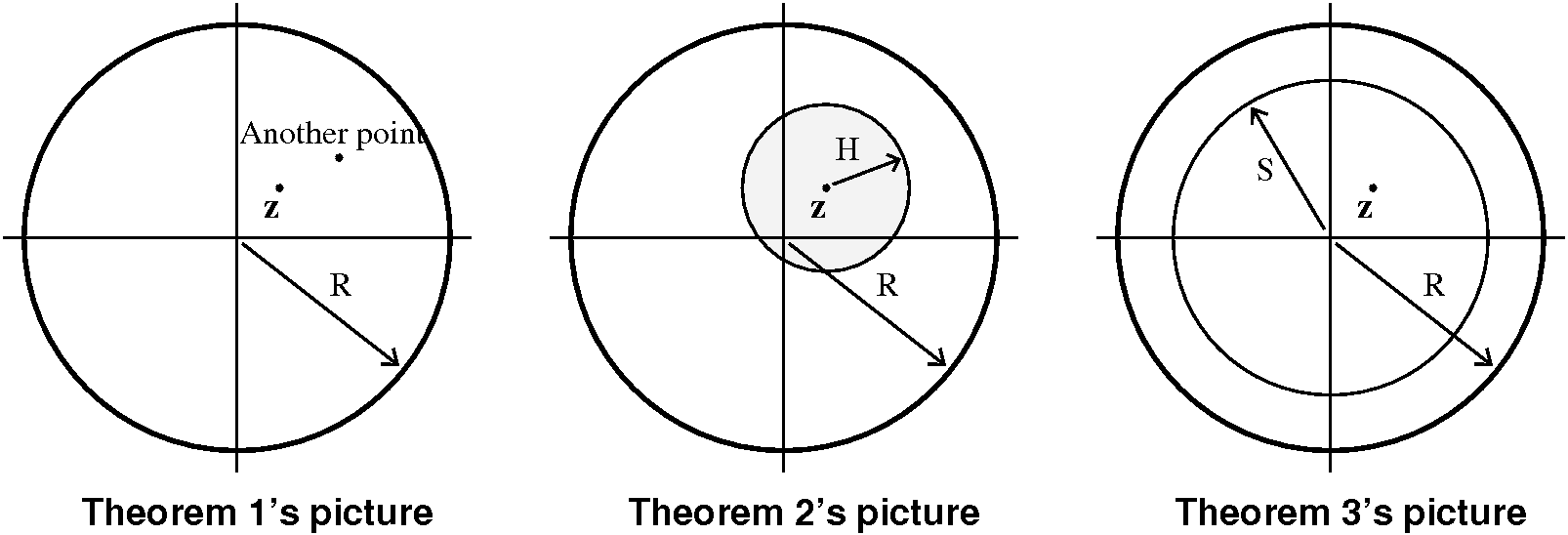
Theorem 1 If f(z)=_n=0a_nzⁿ, then there exists R in [0,], such that if |z|<R, _n=0a_nzⁿ converges absolutely. If S<R, then _n=0a_nzⁿ converges uniformly in when |z|<=S and therefore converge uniformly on all K compact contained in {z with |z|<R}.

R is called the radius of convergence of the infinite series. There is a "formula" called the Cauchy-Hadamard formula for R in terms of the coefficients a_n of the series. It implies standard calculus results such as the Ratio Test and the Root Test. It is also generally strikingly ineffective in actually determining a radius of convergence!

Proof Take R=sup{|z|: sup_n>=0 |a_nzⁿ|< }. Certainly 0 is an "eligible" number, so the sup is taken over a non-empty set.

If R>0, take z with |z|<R. Then there exists z₁ with |z₁|<R and |z|<|z₁|. Let A=sup_n>=0|a_nz₁ⁿ|<. Thus
|_n=0a_nzⁿ|=<_n=0|a_nzⁿ|=_n=0|a_n(z/z₁)ⁿ(z₁)ⁿ|=<_n=0|(z/z₁)ⁿ|A<. The series for z converges absolutely, and therefore converges.

Now take S<R. Suppose we consider z with with |z|=<S. Then |a_nzⁿ|<=|a_n|Sⁿ. We may apply the Weierstrass M-test and get uniform convergence in the closed disc of radius S. Notice that if K is a compact subset of the open disc of radius R, then K is covered by the sequence of open discs of radius R-(1/n), and therefore (finite subcover!), K is contained in one of those discs, and we can take S to be that R-1/n. So there is uniform convergence on any compact subset of the disc of radius R.

Theorem 2 If f=_n=0a_nzⁿ, then f is holomorphic in D_R(0) (R as defined previously) and f´(z)=_n=0na_nz^{n-1}. (So the latter infinite series converges also in D_R, and its sum is the derivative of f).

Proof First let us recall _n=0na_nz^n-1 converges in D_R(0) (you can refer to some textbooks or look very carefully at what we will do.)

Then let us calculate lim_h-->0(f(z+h)-f(z))/h carefully. We will see that the limit exists equals _n=0na_nz^n-1. Fix some H>0, so that |z|+H<R. We will consider h in C with |h|<=H. Then f(z+h)=_n=0a_n(z+h)ⁿ=_n=0a_nk=0ⁿ(Cⁿ_k)z^n-kh^k. This series in h converges absolutely and uniformly when |h|<=H (consider that if we replace z by |z| and h by |h| it just becomes the power series for f(|z|+|h|) (with an expansion using the Binomial Theorem) inside the radius of convergence.

Now define Q_z(h)=(f(z+h)-f(z))/h=_n=0a_nk=1ⁿ(aⁿ)z^n-kh^{k-1}.

You can compare this series to the series for f(z+h). It is almost the same (there is a multiple of h missing and one other term). But if the series for f(z+h) converges then this series is first, a subseries (omit the hⁿ terms in f(z+h), and then, a division by h. So by comparison, this series also converges absolutely and uniformly.

Therefore Q_z(h) is a continuous function of h for |h|<H. So lim_h-->0Q_z(h)=Q_z(0). And if you look carefully, you will see that Q_z(0) is the series we wrote for f´(z). Please notice that we've shown the series converges at least for all z in D_R(0)

Corollary If f(z)=_n=0a_nzⁿ converges, then a_n=fⁿ(0)/n!.

Proof Repeatedly differentiate and evaluate the power series. This corollary essentially states that a convergent power series is the Taylor series at the origin of the function which is the sum of the power series.

Theorem 3 If f is holomorphic in D_R(0),then there exists a sequence {a_n}_n=0 of complex numbers so that f(z)=_n=0a_nzⁿ for all z in D_R(0).

Proof Since |z|D_S(0), the correctly oriented (counterclockwise!) boundary of the circle of radius S centered at 0. Then (the Cauchy Integral Formula!) f(z)={1/(2Pi i)}_s[f(w)/(w-z)]dw. But 1/(w-z)=(1/w)[1/(1-{z/w})]=(1/w)_n=0(z/w)ⁿ. This series converges uniformally on D_S(0), so that we can interchange sum and integral. Therefore f(z)={1/(2Pi i)}_sf(w)/(w-z)dw=_n=0{1/(2Pi i}(_sf(w)/(w^{n+1}dw)zⁿ. Notice (by Cauchy's Theorem) each of the coefficients {1/(2Pi i}(_sf(w)/(w^{n+1}dw) of the power series does not depend on the radius: the value will be the same for any S between 0 and R. So the power series representation is the same for any z in D_R(0).

Corollary fⁿ(0)=n!/(2Pi i)_sf(w)/(w^{n+1}dw where s is the boundary of any circle around 0 inside D_R(0).
We actually already proved this earlier in the course, when we differentiated functions defined with (w-z)^-k as an integral kernel.

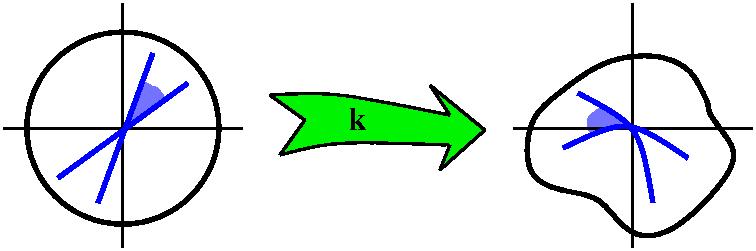
MAJOR RECOGNITION All of the definitions of "holomorphic" are equivalent. That is, suppose f:U-<C, where U is a open domain in C. Consider these statements.

• f=u+iv, u,v are in C¹(U) and u_x=v_y and u_y=-v_x (Cauchy-Riemann equations).
• f is a C¹ mapping from U to R², and either the Jacobian of f has all entries 0 or f is directly conformal at each point (in the sense of the homework assignment: angles between curves in the domain and range are preserved).
• lim_h-->0(f(z+h)-f(z))/h exists for all z in U.
• f has a local power series expression at all points of U. (This turns out to be logically identical to: f has a power series expansion centered at every point, and the radius of convergence of the expansion is at least the distance to the boundary of U.)
• Suppose f is in C⁰(U). If R is any closed rectangle contained entirely inside U (the boundary and the interior), then _Rf(z)dz=0.
• Suppose f is in C²(U), Re f=0 & Im f is a homonic conjugate of Re f.
• f is C & f´ exists.

Morera's Theorem Suppose U open and connected in C and f is a continuous complex-valued function defined on U. Suppose that for all all rectangles R with R contained in U (R means the rectangular box with its inside!) we know _Rf(z)dz=0, then f is holomorphic in U.

PICTURE HERE! Proof The idea is to define a holomorphic F in U so that F =f. Then by results just done today, the derivative f must be holomorphic.

We need only define F "locally". That is, just consider f on an open disc in U. We define an antiderivative F in that open disc. The method is something we've already done several times. Define F(z) to be the line integral from the center of the circle along half the boundary of a rectangle ending at z. Depending upon which half-rectangle you take, each of the partial derivatives is easily seen to be equal to f. Since the two paths give the same value (that's the key hypothesis!) the results must match up which verifies the Cauchy-Riemann equations. This argument is given in detail on page 73 of the text.

It is also true that we didn't verify all details of the following, which showns that we need not assume continuity of f´ in the definition of holomorphic.

Goursat's Theorem If for all z in U, lim_h-->0(f(z+h)-f(z))/h exists,then f is holomorphic.

We will verify this next time using Morera's Theorem.

For Borel's theorem, please see here. For complex analysis, the most important and interesting fact is in the very last paragraph on the third page. I thought more about the proof presented of Borel's Theorem over the weekend. I can now present a proof that is one quarter the length, with much less insight. (Think vertically instead of horizontally!) I will mention this in class. Which proof is "better"? What is "better"?

Suppose we have a C function on [0, inf). From Borel's theorem, we can extend this to a C function on the reals. This result is useful in differential topology, when one might want to "patch together" C functions.

Let {f_n} be a sequence of functions. Let S_n,k=sup|f_n(x)-f(x)| where the sup is over x in [-k,k]. Let S_n,k,j=sup|f^(j)_n(x)-f^(j)(x)| where the sup is over x in [-k,k]. We say f_n-->f is locally uniform if S_n,k-->0 as n--> for all fixed k. We say f_n-->f (in C) is locally uniform if S_n,k,j-->0 as n--> for all fixed j, k. The sequence f_n(x)=x/n shows that these two are not the same. Structural fact: if {f_n} are C⁰ and f_n-->f locally uniformly, then f is C⁰. Also, if {f_n} are C and f_n-->f locally uniformly in C, then f is C.

A norm on a vector space V is a function from V to R such that for vectors v,w and real a:
    i) ||v||>= 0 with equality iff v=0.
    ii) ||av|| = |a| ||v||
    iii)||v+w||<=||v||+||w||.

We can define a metric d by d(v, w)=||v-w||. C functions are a vector space, and we would like a metric such that d(f_n, f)-->0 iff f_n-->(C) f is locally uniform. Unfortunately, no such vector space norm exists with these properties. But we do have a metric, loosely defined by d(f,g)=(1/2^sizeS_X(f-g)/(2^(-something)·(1+S_X(f-g))) where the sum is over some countable enumeration of X,which is triples n,k,j and the size is just the index of the enumeration variable. It is not at all obvious that there is no norm consistent with the metric space structure given by this d. And, honestly, some thought is needed to see that the d(f,g) defined coincides with locally uniform convergence of functions and all of their derivatives. The "structure" of C(R) along with d(f,g), which provides a complete metric on the vector space, with a neighborhood basis of convex sets, is called a Frechet space.

In the case of R and C, locally uniform convergence is the same as uniform convergence on all compact subsets. That's because R and C are locally compact. The convergence is actually more often called uniform convergence on compact subsets (ucc).

Returning to complex analysis, consider all polynomials in z, C[z}. C[z] is well-understood (all finite sums of monomials, or, multiplicatively, assuming C is algebraically closed (!), the product of linear polynomials). Next consider all power series in z, C[[z]]. This is sort of all complex sequences. It has a ring structure where addition is coordinate by coordinate, but multiplication is somewhat weird when considered abstractly. The product of two sequences of complex numbers, (a_n)_n>=0 and (b_n)_n>=0, is a third sequence, (c_n)_n>=0, with c_n=_j=0ⁿa_jb_n-j. The product is not the coordinate-wise product. This is inherited from the intermediate ring, which we will be studying, the ring of convergent power series. It is our goal to find a subring of the power series in z such that all functions in the subring are holomorphic, and any holomorphic function can be locally represented as a series in the subring.

We will prove the following fundamental fact: Given _r=0a_rz^r, there exists an R in [0,] such that if |z|>R, then the series divergences, and if |z|<R, the series converges absolutely. Furthermore, if S "Examples" (The reason for the quotes is that a naive person would need to think quite a bit to verify them!).
    a_r=r!, then R=0.     a_r=1, then R=1.     a_r=1/r!, then R=.

The motivation for this comes from geometric series. If r<1, then _n=0wⁿ converges locally uniformly to 1/(1-w) when $|w|<1.

Proof 1+w+w²+...+w^k=(1-w^k+1/(1-w) when w is not 1. But lim_k-->w^k+1=0 for |w|<1, and this limit is uniform in compact subdiscs of the unit disc. Therefore, since |_n=0^Nwⁿ|<=_n=0^N|w|ⁿ, we're done (Weierstrass).

There are several methods for specifying the R, called the radius of convergence, for _r=0a_rz^r. There is a classical formula (which sometimes provides very little information) called the Cauchy-Hadamard formula. Here R will be the following more irritating number, which has more easily discerned information:
R=sup of z in C with sup_r>=0|a_rz^r|<. R is the sup of those z s for which the individual terms of the power series are bounded. Notice that if z=0, the terms are always bounded (all but the first are 0, after all!). So the sup is taken over a non-empty set of complex numbers.

First, the lecturer berated us for our solutions to #2 (most of the students anyway). The text should have indicated that the problem was an explicit method for getting an antiderivative of a holomorphic function in a disc (indeed, in a star-shaped open set). The "recipe" given can be independently verified (with FTC or equivalent tools) as an antiderivative. Most students quickly solved the problem by appealing to the already known result that, in discs, holomorphic functions have antiderivatives. The problem in the text uses a now-standard technique for verifying what's called the Poincaré Lemma about closed and exact differential forms. One reference is Spivak's text, Calculus on Manifolds.

The overall goal of this week is, almost, to turn 503 into an algebra course. Holomorphic functions are a rather peculiar collection of rings. But this is postponed, and we will have an excursion (digression?) into some associated topics.

The scribe would like to note that a reference for the well-known material of the lecture is Rudin's Principles of Mathematical Analysis, Chapter 6(?).

Last time, we showed that O(U), the holomorphic functions defined on an open subset U of C, is actually a subset of C(U). Before giving another characterization of holomorphic functions, maybe we should learn a bit about C, and, on the way, review convergence ideas for functions. It is interesting to note that the convergence ideas we will discuss, which are now so clear to define and use, were historically arrived at with numerous stumbles (!) and errors (!!). A century and a half ago, the "correct" ideas for convergence were not totally clear. The lecturer hopes that this is an encouraging statement to students at the start of their research careers. We will consider several examples of functions in C(R).

Begin with A ...
We create A in C(R), defined piecewise: A(x)=0 if x<0 and A(x)=e^-1/x if x>0. Also, A(0)=0.

Is it "clear" that A is C? The continuity of A at non-zero x should be clear. When x=0, we need to verify that lim_x-->0⁺A(x)=0. This is the same as lim_x-->0⁺e^-1/x=0, but if 1/x=w, we have the limit lim_w-->+e^-w which is certainly 0. (The reason for going through this is so that a more complicated limit, coming up, will be easier.)

Let's try for C¹: A´(x) certainly exists for x not zero. When x<0, A´(x)=0, and when x>0, A´(x)=e^-1/x(1/x²). If we wish to consider A´(0), we should look at the official definition. Since A(0)=0, we have to consider lim_x-->0A(x)/x. As x-->0^-, this is clear 0. What about from the right? Well, lim_x-->0⁺A(x)/x is the same as lim_x-->0⁺e^-1/x(1/x) and this is the same as (with 1/x=w) lim_w-->+we^-w=lim_w-->+w/e^w which, with L'Hôpital's Rule, is 0.

Therefore A is C¹. We could continue or think inductively. To go from C^k to C^k+1, realize that a formula for A^(k)(x) when x>0 looks like e^-1/xP(1/x) where P is some one variable real polynomial. The same trick as before (change variables, use L'Hôpital) shows that lim_x-->0⁺e^-1/xP(1/x)=0. So A is C.

Go on to B Now define B with B(x)=A(x)·A(1-x). B is surely C since it is the product of C functions. These functions are also non-negative, so B is non-negative. And the support of B, sometimes abbreviated supp(B) and referring to the closure of the set where B is not 0, is [0,1]. B is a C bump function.

And even to C! We'll define C with the equation C(x)=-xB(t)dt. Since B is 0 for x<0, the function will be the same if we define it with any non-positive lower bound. Since C´(x)=B(x), we know that C is constant for x<0 and for x>1. Since B is non-negative (and positive inside [0,1]), the latter constant is positive. We can multiply C by a positive constant so that C(x) will be 1 for x>1.

And now D, which is for Digression
We need this to clarify some previous comments. Define D, which is in C(R), by D(x)=xC(x). This function is 0 for x<0, and is strictly increasing (look at its derivative!) for x>=0. We can use this function to define a C parameterized curve in R².

Consider s:R-->R² defined by s(t)=(D(t),D(-t)). We see that s is C and is also one-to-one (the two D's work to show that in different parts of the domain). However, s is a "bad" curve, or at least unintuitive. The image of s is L. By that we mean the union of the positive x-axis, the positive y-axis, and 0. The image of this "smooth curve" seems to have a corner. The problem is that the parameterizing variable doesn't even see (?) the corner. It's velocity vector is 0 there. Think about this.

People who study differential geometry don't like this, so a slightly different kind of curve is used:
Definition s is a regular curve if is C and s´ is never zero.
L is not the image of a regular curve. This is not totally obvious (one verification uses the {Inverse/Implicit} Function Theorem). Students should try to verify this, and if they cannot, please see the instructor.

Partitions of unity
The following was mentioned with no proof. The proof takes some careful verification (see any reasonable differential topology text), and really would be too far from our discussion of complex analysis. If {U_a}_{a in A} is an open cover of R, then there is a C partition of unity which is subordinate to {U_a}_{a in A}: a collection of functions {f_a} so that:

Each f_a is C, 0=<f_a(x)<=1 for all x in R, and supp(f_a) is contained in U_a. The supports are locally finite (each x in R has a neighborhood in which at most finitely many f_a's are not 0) and _{a in A}f_a(x)=1 for all x in R.

Maybe a true smooth "bump"
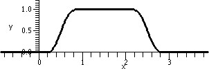
Finally, the last in this sequence of examples. Look at C, defined previously. For x>1, C is constant. That constant, by the way, is about 0.007029858407.
Who cares? We should remember that The purpose of computing is insight, not numbers as Richard Hamming wrote. There's no insight in this number. It is the slope of the D function for x>1. Sigh.
So consider the smooth function defined by the formula C(x)C(3-x) divided by the square of that constant (we've got to adjust two copies of C). A graph of this function is shown to the right. You don't have to like this function. In fact, I am almost sure that almost no mathematician whose career was earlier than the 20^th century would like this function.
Properties The support of this C function is [0,3], its values are all non-negative, and it is 1 on [1,2]. It is increasing on [0,1] and decreasing on [2,3].

I hope that it is clear by scaling, etc., we can do the following: given any a<b<c<d, create a C function whose suppose is [a,d], which is always non-negative, which is 1 on [b,c], and which is increasing on [a,b] and decreasing on [c,d]. These are called smooth bump functions.

A theorem, finally!
This result is an indication that there are so many C functions, and that they can do almost anything!

Theorem (E. Borel) Given any sequence of real numbers {a_n}, there exists f in C(R) with f⁽ⁿ⁾(0)=a_n for all n>=0.

"Proof" f(x)=_n=0(a_n/n!)xⁿ. not quite...
The reason for "not quite" is that the series need not converge for any value of x except 0. But now we have an excuse (!) to study such convergence.

Questions of convergence ...
Suppose X is a metric space. Then {x_n}, a sequence in X, converges to x (its limit is x) if for all e>0, there exists N(e) such that if n>N(e), then d(x_n,x)<e. This definition requires us to "know" somehow the limit, x, of the sequence. We can supplement it with an "internal" criterion for convergence, depending only on the sequence: A sequence {x_n} is Cauchy if for all e>0, there is M(e) such that if n₁, n₂ > M, then d(x_n1,x_n2)<e. Every convergent sequence is Cauchy, but the converse is not necessarily true. The Cauchy idea is useful (it is usually called the Cauchy criterion), so we define: a metric space is complete if all Cauchy sequences converge. My favorite complete metric spaces are R and C and a few other function spaces we will meet later.

Convergence of functions
Let {f_n} and f be functions from X to R (or C).
f_n converges pointwise to f if for all x in X, lim_n-->f_n(x)=f(x). {f_n} converges uniformly to f if for all e>0, there exists N such that if n>N, then |f_n(x)-f(x)|<e for all x.
Uniform convergence implies pointwise convergence. The converse is not true. For example, the sequence xⁿ converges pointwise but not uniformly to 0 on the open interval (0,1).

Big result
We care about this because of the following proposition:
Theorem If {f_n} is continuous from (X,d) to R (or C) and {f_n} converges uniformly to f, then f is continuous.

Proof We need to show that, given e>0 and x in X, there is d>0 so that if y is in X and d(x,y)<d, then |f(x)-f(y)|<e. Since {f_n} converges uniformly to f, there is N so that if n>N, |f_n(w)-f(w)|<e/3. Fix one such n greater than N. That f_n is continuous on X, and more precisely, continuous at x in X, so there is d>0 so that any y in X with d(x,y)<d must satisfy |f_n(y)-f_n(y)|<e/3.
Now consider what happens if d(x,y)<d:
|f(x)-f(y)|=<|f(x)-f_n(x)|+|f_n(x)-f_n(y)|+|f_n(y)-f(y)|<e/3+e/3+e/3=e
and we are done.

Pointwise convergence does not generally "transmit" continuity: consider xⁿ on [0,1]. The pointwise limit is a function which is 0 for x<1 and 1 for x=1: not continuous.

{f_n} converges locally uniformly to f if for all x in X, there exists a neighborhood N_x such that f_n|_Nx converges uniformly to f|_Nx.

Proposition A locally uniformly convergent sequence of continuous functions has a continuous limit.

Now on to series!
_j=0f_j(x) converges pointwise if the sequence {F_N} converges pointwise, where F_N(x)=_j=0^Nf_j(x) (a partial sum of the infinite series).

_j=0f_j(x) converges uniformly if the sequence of partial sums, {F_N} converges uniformly.

_j=0f_j(x) converges locally uniformly if the sequence of partial sums converges locally uniformly.

_j=0f_j(x) converges absolutely if _j=0|f_j(x)| converges pointwise.

Of course, convergence does not imply absolute convergence (_j=0(-1)ⁿ/n), but the converse is true: absolute convergence does imply convergence (this uses the Cauchy criterion, and students should be able to write out the argument).

Weierstraß
Theorem (Weierstrass M-Test) Suppose that {a_j} is a convergent series of non-negative numbers: _j=0a_j<. Also suppose that there exists M>0 such that |f_j(x)|=<Ma_j for all x in X. Then _j=0f_j converges uniformly and absolutely for all x in X.

How about the proof?
Now we play around with the function for "Proof" of Borel's Theorem. I'll use CHI_A to be the characteristic function of A, a subset of R, so CHI_A(x) is 1 if x is in A and 0 otherwise.
Consider f(x)=_j=0{(a_n/n!)xⁿ}·(CHI_[-rn,rn](x)), where I_n=[-r_n,r_n] is the interval whre |(a_n/n!)xⁿ|<1/2ⁿ (there is such an interval, since the monomial function is 0 at 0). Then, the series describing f converges uniformly and absolutely. However f is not C⁰. So we need to "cut off" things more smoothly -- we need to introduce smooth convergence multipliers.

Suppose b is a specific fixed smooth bump function: b(x) is 0 for |x|>1 and 1 if |x|<1/2. Also, b is between 0 and 1 otherwise, even increasing in [-1,-1/2] and decreasing in [1/2,1].

Consider f(x)=_j=0{(a_n/n!)xⁿ}·b(r_nx). Each summand is C and the series converges absolutely and uniformly (comparing with a geometric series with ratio 1/2!). So f is C⁰, and f(0)=a⁰. What the heck happens when we differentiate? We need a theorem, maybe.

Differentiating a sum
Proposition Suppose that {f_n} is a sequence of C¹ functions on R with f_j converging uniformly to f and f_j´ converging uniformly to g. Then f is C¹ and f´=g.

Proof We'll use the fact (previously mentioned in connection with the ML inequality) that integration can be "exchanged" with limits of uniformly convergent sequences of functions. Here we know f_j(x)-f_j(0)=₀^xf_j´(t)dt by FTC. Now take lim_j-->. The result (after the mentioned interchange!) is f(x)-f(0)=₀^xf´(t)dt=₀^xg(t)dt
and now the "other" (?) part of FTC (differentiability of a variable upper bound in an integral) implies that f is differentiable, and that its derivative is g.

You may notice that we don't really use all the information about the convergence of f. The conclusion still is valid if we only know f_j(0) converges to f(0).
But then we can only get "out" that the sequence of functions, {f_j} will converge locally uniformly to f. EXAMPLE?

The discussion of the proof of Borel's Theorem will continue, and then we will return to complex analysis.

Mr. Kim's (justified) complaint
In the proof of Cauchy's Theorem from last class, we showed that given two C⁰ curves in U which are homotopic in U, and a function f holomorphic in U, the line integral around the two curves is equal.

To do this, we split up the homotopy diagram into tiny rectangles, around which we knew the integrals were 0. The sides of the rectangles in the interior canceled each other out, leaving the integrals along the sides of the homotopy diagrams. The line integrals at the top and bottom of the diagram are the two we claimed to be equal. But Mr. Kim wondered, what about the integrals on the sides of the diagram? Where did they go?

We neglected to take note of the fact that since the homotopy H was set up so that H(0,t)=H(1,t) for all t, meaning the sides of the diagram are curves with the same endpoints. Since they are traversed in opposite directions, they create a closed curve, around which we know the integral is 0. And that is where those integrals went.

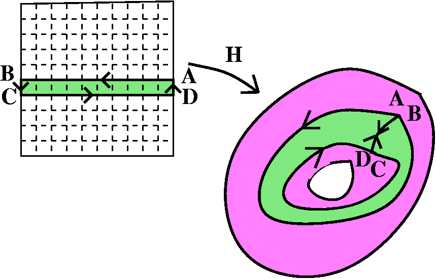
The accompanying diagram shows the situation. The ABCD integral is 0 using the reasoning of the last lecture. The integrals from B to C and from D to A cancel, since they are pointwise the same curve but described in reverse order. Therefore the integral from B to A is equal to the integral from C to D (all the ordering works!).

An analysis course has inequalities. Why wasn't the most important inequality in complex analysis stated and proved?
The ML Inequality Suppose s:[a,b]-->C is a C¹ curve, and f is continuous on s([a,b]). Then |_sf(z)dz|<=ML, where M=(sup_{z in s([a,b])}|f(z)|) and L=length of s, which is |s´(t)|dt.

Proof |_sf(z)dz|= |_a^b|f(s(t))s´(t)dt|<=_a^b|f(s(t))| s´(t)|dt<= (sup_{z in s([a,b])}|f(z)|)|s´(t)|dt. (Sort of L¹ and L.)

This works if s:[a,b]-->C is a piecewise C¹ curve.

An application of the above inequality:
Proposition Suppose {f_j} is a sequence of continuous functions on s([a,b]) and f_j converges uniformly to f on s([a,b]). Then lim_{j--> s}f_j(z)dz=_slim_j-->f_j(z)dz.

This is the only limit interchange theorem in the course. I hope.

Here's the proof. What's the theorem?
Proof Suppose Q(z)=_sA(t)/(t-z)ⁿdt, where A is C⁰ on the image of s, and z is not in the image of s. Take h so small that if |h|<=E, then |z+h| is in U.

(Q(z+h)-Q(z))/h=_sA(t)((1/h)(1/(t-z-h)ⁿ1/(t-z)ⁿ)dt=_s(A(t)/h)((t-z)ⁿ-(t-z-h)ⁿ)/[(t-z-h)ⁿ(t-z)ⁿ]dt. A(t) is not "where the action is".. So let's look at where the action is. (Here C_n,j is the n,j binomial coefficient.)
(((t-z)ⁿ-(t-z-h)ⁿ)/[(t-z-h)ⁿ(t-z)ⁿ]=((t-z)ⁿ_j=0ⁿC_n,j(t-z)^n-j(-h)^j)/(h(t-z-h)ⁿ(t-z)ⁿ=_j=1ⁿC_n,j(t-z)^n-j(-h)^j)/[h(t-z-h)ⁿ(t-z)ⁿ]=_j=1ⁿ(C_n,j(t-z)^n-j(-h)^j-1)/[(t-z-h)ⁿ(t-z)ⁿ].

In this last expression, there are a few things to note. We treat z as fixed. h is in the closure of the disk of radius E centered at the origin. t is s(w), for w in [a,b], i.e., t is in s([a,b]). Treating this last expression as a function F(h,t), these observations lead to the conclusion that F(h,t) is continuous.

More precisely, F:(The closure of the disk of radius E centered at the origin)xs([a,b])-->C is continuous. Since the domain of F is a compact set, F is uniformly continuous: given r>0, there exists d>0 such that if |h₁-h₂|<d and |t₁-t₂|1,t₁)-F(h₂,t₂)| What is F(0,t)? F(0,t)=(n(t-z)^n-1)/(t-z)²ⁿ. F(h,_) converges uniformly to F(0,_) as h goes to 0, where _ is some t in s([a,b]). So we may interchange limit and integral: lim_h-->0sA(t)((1/h)(1/(t-z-h)ⁿ)(1/(t-z)ⁿ)dt=_slim_h-->0A(t)F(h,t)dt=_sA(t)F(0,t)dt.

What's the theorem?

Theorem Suppose s:[a,b]-->C is a piecewise C¹ curve, and A is continuous on s([a,b])). Define Q(z)=_sA(t)/(t-z)ⁿdt. (Here n is a natural number.) Then Q is holomorphic on C\{s([a,b])} and Q´(z)=_snA(t)/(t-z)ⁿ⁺¹dt. (A homework problem was a version of this!)

The most important specific use will be when A(t)=1, n=1, s a closed curve. Then Q/(2Pi i) is the "winding number". We will discuss this later.

Recall the Cauchy Integral Formula: Given an open set U, with a closed disk with radius r and center p contained in U, f holomorphic on U, and z in the interior of the disk, then f(z)=(1/2i)_{bdry of the disc}(f(t)/(t-z))dt.

Using the above Theorem combined with this fact, we get a
Cauchy Integral Formula for Derivatives. Given the same hypotheses as the Cauchy Integral Formula, we get that f is C on U, f⁽ⁿ⁾ is holomorphic on U for all n, and f⁽ⁿ⁾(z)=n!/(2Pi i)_{bdry of the disc}(f(t)/(t-z)ⁿ⁺¹)dt.

But wait, here's something curious. From above, we get f´(z)=(1/2Pi i)_{bdry of the disc}(f(t)/(t-z)²)dt. But also we could use the Cauchy Integral Formula directly: f´(z)=1/(2Pi i)_{bdry of the disc}(f´(t)/(t-z))dt (since f´ is also holomorphic). So are these the same? Integration by parts should convince you that yes, they are.

Two Awesome Consequences

#1
Suppose we have u(x,y), u:U-->R, U open in C, u is C²(U), and u=0. Take p in U with E>0 so that the open disk of radius E with center p is contained in U. Suppose u=0 in the open disk of radius with center p. This means there _xxu+_yy=0. Then we saw earlier that there exists a function v that is C² in the disk so that u+iv is holomorphic on the disk (v is a "harmonic conjugate" of u). From what was just discussed we know now that u+iv is C on the disk, so u is C in the disk and Conclusion u is C on all of U.

This is a case of Weyl's Lemma. On a related note, here is an oral exam at the Courant Institute: Can you prove Weyl's Lemma? How many ways?

#2
Suppose U is a simply connected open set in C. Now we know if f is holomorphic on U, there exists an F holomorphic on U such that F´=f. We proved this on an open disk using the Fundamental Theorem of Calculus. We can do this on U because of the simple connectedness. Suppose s is a curve "from" a fixed z₀ to z. If F(z)=_sf(z)dz, we know F(z) does not depend on our choice of s since any other curve with the same endpoints will combine with s to create a closed curve, which is homotopic to a point ("simply connected"!). So we change s to a curve that we can use FTC on (it would end up with a vertical line segment or a horizontal line segment).

Given U simply connected and open in C and an f holomorphic in U which never vanishes, there exists a function L holomorphic in U such that e^L(z)=f(z), and for all n in the natural numbers, there exists a function h holomorphic in U such that hⁿ=f. You may recall that we gave a proof of this for the unit disk, but not very well. Well, with only one huge hole. We know more now, specifically that f has a holomorphic derivative on U, so we can do it again and be right this time. Remember the idea was to define g(z)=f´(z)/f(z). g is holomorphic, since f and f’ both are and f never vanishes. This means there is a G(z) such that G´(z)=g(z). Then exp(G)=f (or almost, with possible correction by a multiplicative constant). Also, (exp(G))´=(f´/f)exp(G), compute the derivative of f/e^g, etc. G is the L promised above.

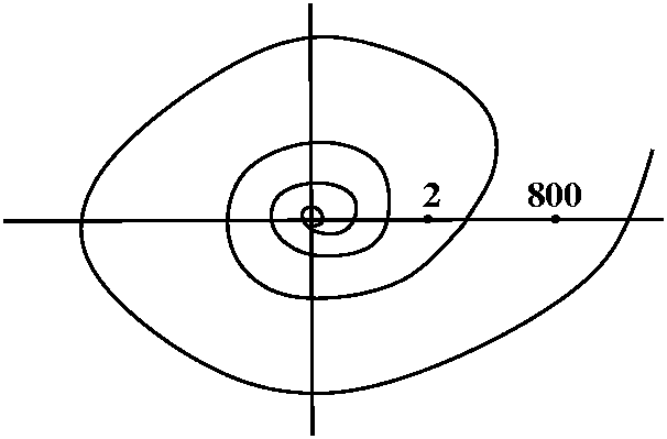Example
Look at the polar curve D given by the equation r = e in R^². This is a equiangular spiral. It spirals around the origin infinitely often outside of any disc. As z-->0, it spirals infinitely often around the origin also. The curve and the origin together, DU{0}=X, is closed in R², so U=C\X is open in C. z is holomorphic in U, z is not 0 in U, and U is simply connected. (Clearly. Well okay, a little more on this later.) So by above, there exists a function L such that exp(L(z))=z in U: e^L(z)=z. We'll write L(z)="log"(z) here.

Lets look at this "log"(z). Since exp is 2Pi i periodic, given one "log" there will be infinitely many others. But we can adjust or select so that "log"(2)=log(2), a value of the standard, ordinary log. But when you follow the spiral around to get to another value on the real axis, you gain 2Pi i, e.g. "log"(800)=log(800)+2Pi i.
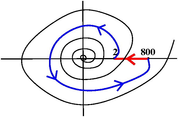Let's give the acute reasoning of Ms. Naqvi here. So let's go from 2 to 800. One way of doing this is to get a path, s, from 2 to 800 in U, and then "log"(800)=log(2)+_s(1/z)dz. But follow that path with the line segment from 800 to 2 on the real axis. This is a curve around 0, and by Cauchy's Theorem (it is homotopic to a circle around the origin) the integral over the curve followed by the line segment of 1/z is 2Pi i. The line segment integral is a standard real integral, and its value is log(2)-log(800). It goes "backwards", so we indeed do get "log"(800)=log(800)+2Pi i.
Yes, the picture is distorted.

"log" will give you "sqrt" in U, defined by "sqrt"(z)=e^{((1/2)"log"(z)}. "sqrt"(2) will be sqrt(2), but "sqrt"(800) will be -sqrt(800) since e^Pi i=-1. "sqrt" will alternate in sign on each piece of the real axis as you go out to + or to 0. The sign changes each time the spiral is crossed.

Classically speaking, we have just shown that there is a branch of log in U. And U's simple connectedness follows from the fact that the image of any curve in U is compact. So any curve will be bounded away from 0 and away from "" -- it will be in between a finite number of loops of the spiral.

Homework remarks
Please note that problem 2 of assignment 1 provides yet another characterization of holomorphicity. A C¹ function is holomorphic if its Jacobian is either identically 0 or if it locally is orientation preserving and preserves angles between curves (it is "directly conformal" [the adverb "directly" is frequently omitted]). This is because the Jabobians of such mappings implicitly imply the Cauchy-Riemann equations.

Also please note that A+B<C+D does not provide enough information to conclude that A<B. Sigh.

The main goal of this lecture is to prove Cauchy's Theorem, so we start at the very beginning, by given a definition of the integral over a closed C^0 curve:

Basic hypothesis U a open subset of C, f a holomorphic function in U and s:[a,b]->U a C⁰ curve in U

And we want each of the following items to be possible

1. A partition of the [a,b] interval: a=t₀<t₁<...<t_n-1<t_n=b such that there exists a collection of open discs in U: D_rj(z_j) such that s([t_j-1,t_j]) is contained in D_rj(z_j) for all j=1,...,n.
2. A collection of holomorphic antiderivatives of f in each disc: F_j holomorphic in U and (F_j)´ = f in D_rj(z_j).
3. And this "thing": F₁(s(t₁))-F₁(s(t₀))+...+F_j(s(t_j))-F_j(s(t_j-1))+...+F_n(s(t_n))-F_n(s(t_n-1)). This is the "Thing Formula".

We first realize that if we change one of the antiderivatives in one of the discs, ie, we replace F_j by another antiderivative G_j in the definition of the "thing", we obtain the same result, since F_j=G_j+D for some complex constant D, and therefore, F_j(s(t_j))-F_j(s(t_j-1))=G_j(s(t_j))-G_j(s(t_j-1)).

Now, if we select another disc D_Rj(Z_j) instead the original D_rj(z_j) disc, ie, we have s([t_j-1,t_j]) contained in D_rj(z_j) and a antiderivative F_j, and s([t_j-1,t_j]) contained in D_Rj(Z_j) and a antiderivative G_j. In this situation, since both discs are open, the intersection is a non empty, open, convex set (hence connected), therefore we can proceed by selecting a unique antiderivative in the 2 discs (this was a HW problem). The G_j and F_j differ by a constant, as in the previous paragraph.

Finally, if we change the partition, we proceed using the Calc I approach: we only need to prove that this "thing" does not change if we add a new point to the partition.

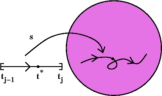So if we add t^* with t_j-<t^*t_j, and we select discs such that s([t_j-1,t^*]) is contained in D_a(z_a), s([t^*,t_j]) is contained in D_b(z_b), with antiderivatives F_a and F_b respectively, we can prove, using the same intersection, open, convex, connected argument used above, that
(F_b(s(t^*))-F_b(s(t_j-1)))+(F_a(s(t^*))-F_a(s(t_j-1)))=F_j(s(t_j))-F_j(s(t_j-1)). (Picture)

We have already seen that if s is a piecewise C¹ curve, the "thing" is equal to the usual value of the integral of f(z)dz on s. Therefore we can say that this "thing" is in fact a good definition of the integral of f over the C^0 curve s: _sf(z)dz.

We return to the main result of this course.
Theorem (Cauchy's Theorem) Given U a open subset of C, a holomorphic function f in U, and two closed C⁰ homotopic curves, s and r, then _sf(z)dz= _tf(z)dz.

Proof Suppose H:[0,1]x[0,1]->U is the C⁰ homotopy between s and t, namely H is a C⁰ function in [0,1]x[0,1] and

1. H(0,t)=s(t) for t in [0,1],
2. H(1,t)=r(t) for t in [0,1],
3. H(s,0)=H(s,1) for all s in [0,1],

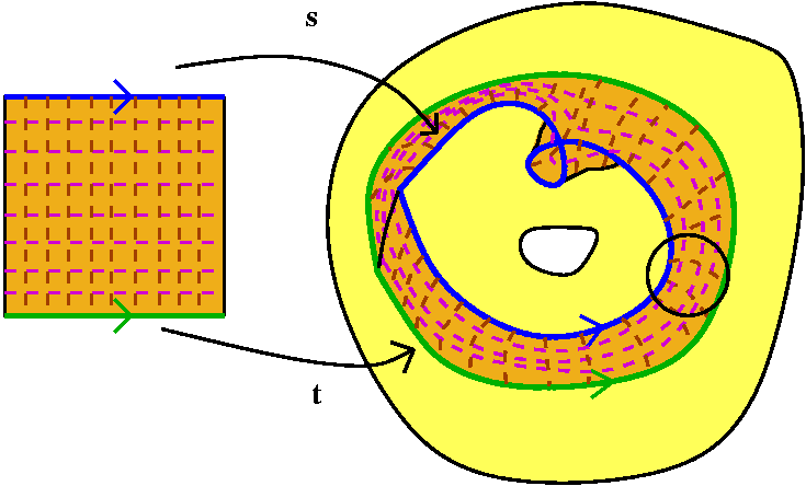The picture to the right is supposed to show the situation. Sigh. It is complicated. The circle shown in U, to the right, is the boundary of a disc enclosing the image of one of the "tiny" rectangles. Good luck in understanding the picture!

Now, we can use the "thing" formula to compute the integral of f over the image by H of the border of S_j. From the formula we note that that integral has to be 0, since it is over a closed curve in a connected region and f has a holomorphic antiderivative in that region (this is why we select the discs and the partition of the unit square).

So if we are smart enough, we can use the fact above to prove that the integral of f over H|{0}x_=s is equal to the integral of f over H|{1}x_=t (It is just a big telescopic sum together with the fact that the homotopy is also a "closed curve", namely, the number 3 of the properties of the homotopy).

In fact, one detail was left out, and thanks to brave Mr. Kim, this will be discussed in the next lecture.

Now some corollaries:

Corollary 1 If s is a closed curve which is C⁰ homotopic to a point in U open set, and f is a holomorphic function in U, then the integral of f over s is equal to 0: _sf(z)dz=0.

Definition U is called simply connected if all C⁰ closed curves in U are homotopic to a point in U.

Examples

1. If U is convex or star shaped, then U is simply connected: For any closed curve s, H(a,b)=az₀+(1-a)s(b) is a homotopy between s and a "curve" which is constantly z₀.
2. C\{0} is open and connected but NOT simply connected: The integral of 1/z over the unit circle is not 0. Since 1/z is holomorphic in C\{0}, this together with corollary 1 shows that the unit circle is not homotopic to a point in C\{0}.

Is any sort of converse true? But we want more theorems. Here is a Possible Theorem For U a open subset of C, s a closed C0 curve in U, and if for every holomorphic function in U, sf(z)dz=0, then s is homotopic to a point. But this is false, since we can provide a counterexample: U=C\{0,1}, and suppose that s is the curve given in the picture, then the integral of any function holomorphic in U over s is 0, but s is not homotopic to a point (this is because U has a non trivial fundamental group, moreover is a free group with two generators a,b, and the s is the curve aba-1b-1.)

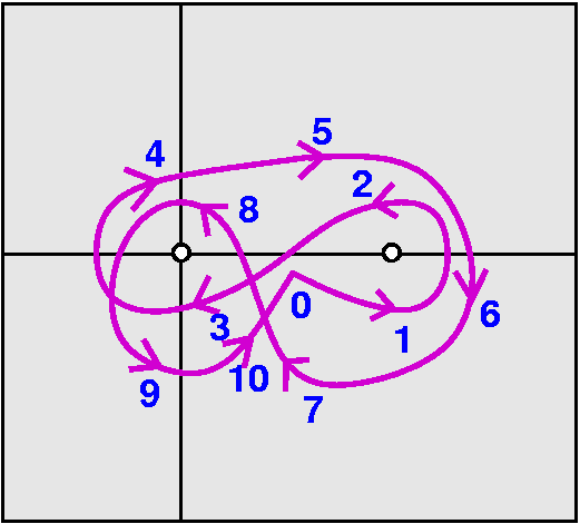
The purpose of the numbers is to help you "see" the curve. The numbers are successive positions on the curve, not values of the parameter. Maybe you can see how a point on the curve would travel. I would like to convince you that if f is holomorphic in C\{0,1} then sf(z)dz=0. The first picture, to the left, shows a region inside the green rectangle with two arrows which indicate how a homotopy would go. It would push the curves into the x-axis at a point between 0 and 1. Because of Cauchy's Theorem, the value of the integral of a holomorphic f around the homotopied curve won't change. In the second picture, to the right, I hope you can "see" that the integral of f around the curve will be 0. There are really four pieces, and if we split the curve into those four pieces, each piece can be homotopied into the reverse of another piece (the curve going backwards). Therefore the integrals will all cancel.
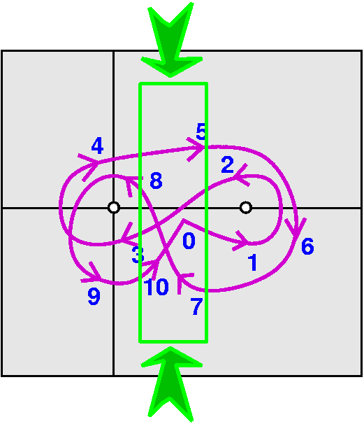
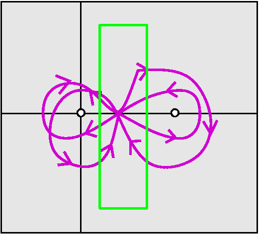
This does not prove that the curve can't be homotopied to a point. I can't do that right now in this course, but maybe (?) this is "clear", since we would somehow have to pull one loop over a hole in order to untangle the curve. This curve is homologous to 0. In fact, homology theory gives a better language for curves and integrals of holomorphic functions -- the Cauchy Theorem has, more or less, a nice converse. For this you need to learn a bit more, and then read a homology version of the Cauchy Theorem (the textbook has this). I presented this homotopy version because I think it is a bit easier to learn. The first homology group of an open subset of C is the fundamental group mod its commutator subgroup. See also the classroom note by Peter Lax in the October 2007 edition of the American Mathematical Monthly. There he describes this situation as one of his favorite oral qualifying exam questions. For those of you who are sophisticates, you know that C\{0,1} has a universal covering space, and the deck transformations of that space "are" the Fundamental Group of C\{0,1}. The mapping from the universal covering space (which can be thought of as C!) can be realized as a specific holomorphic function, called the elliptic modular function. This function is very important in number theory, and, once "constructed", can be used to give a very neat, brief proof of a famous result called the Great Picard Theorem.

Now the also famous
Theorem (Cauchy Integral Formula) Given U open in C, f holomorphic in U, and a disc D_r(p) compactly contained in U, with the boundary curve C of D_r(p) oriented as usual. Then for any z in D_r(p),
f(z)=(1/2Pi i) _C{f(q)/(q-z)}dq.

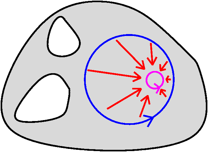Proof Fix z, and define g(w)=f(w)/(w-z). Then g is holomorphic in U\{z}. Next we note that C is homotopic in U-{z} to D, the boundary of a circle of radius v centered at p (v sufficiently small -- such a disc exists since U is open), hence by Cauchy's Theorem the integral of g over C is equal to the integral of g over D. A possible picture of the homotopy is to the right.

Finally, we parametrize D using q=p+ve^it with t in [0,2Pi]. Here is what happens: dq=ve^iti dt and q-z=ve^it so that
_D{f(q)/(z-q)}dq= ₀^2Pif(z+ve^it)i dt.

The significant thing is that the apparant "singularity" in the bottom (the "Cauchy kernel") somehow goes away. Even more magic (?) occurs, because the statement that f is continuous at z is logically equivalent to f(z+ve^it)-->f(p) uniformly for t in [0,2Pi]. Therefore we can exchange limit (as v-->0) and integral to get 2Pi i f(z).

Proposition If f is holomorphic in U, then f is C²(U) and f´ is holomorphic in U.

Proof The initial idea was to write f´ as the limit of (f(z+h)-f(z))/h and then use Cauchy's integral formula, but the class ended just at this point. Hopefully the proof will be completed in the next class period.

And in closing, I think it is important to re-quote Von Neumann: "In mathematics you don't understand things. You just get used to them"

The instructor remarked that when he finally (?) verifies this result, one remarkable consequence will be that C² solutions of _xxu+_yyu=0 will turn out to be C. This is not at all an obvious fact.

Historically, the Laplacian was one of the oldest partial differential operators studied because of its importance in physical modeling. I think an even earlier example of a partial differential operator was this: _xx-_yy (note the very important difference in sign!). Solutions of the homogeneous equation corresponding to this operator (solutions of "the wave equation") are of the form f(x+y)+g(x-y) where f and g are any C² functions of one variable. You can check this easier using the Chain Rule. However, these solutions do not need to be C (this involves what are called "shocks").

So the change from + to - is significant, and that harmonic functions must be C is not at all obvious!

Today we began by computing some line integrals in order to examine some possible truths.

Possible Truth #1 The line integral of any continuous function on any closed curve is 0. (This would be very interesting if it were true and would make much of physics and mathematics unnecessary.)
Counterexample #1 f(z)=1+2z+z(z-bar) integrated clockwise around s, the border of the upper right quadrant of the circle centered at 0 of radius 2. We broke the path sigma into three segments s₁, s₂, and s₃. s₁ was the line segment from 0 to 2. s₂ was the circular arc from 2 up to 2i. s₃ was the line segment from 2i to 0. We know that _sf(z)dz=_s1f(z)dz+_s2f(z)dz+_s3f(z)dz.

_s1f(z)dz=₀²1+2t+t²dt=t+t²+t³/3]₀²=2+4+8/3.

_s2f(z)dz=₀^Pi/2(1+4e^it+4)2ie^itdt=2i ₀^Pi/24e^2it+5e^itdt=2i((4/(2i))e^2it+(5/i)e^it)]₀^Pi/2=(-4+10i)-(4+10)=-18+10i.

_s3f(z)dz=-₀²(1+2it+t²)i dt=-i(t+it²+t³/3)]₀²=-i(2+4i+8/3)

It is important to notice the way that each of the parametrizations of the curves was chosen. The first straight line segment was given by t on the interval [0,2]. The curve was given by 2e^it on the interval [0,Pi/2]. The third was given by i t on the interval [0,2]. We needed to multiply the integral by -1 so that we were integrating the line segment from 2i to 0 rather than the line segment from 0 to 2i.

All this gives us sigma f(z)dz = 2+4+8/3-18+10i-i(2+4i+8/3). This is not equal to zero, so Possible Truth #1 is false.

Possible Truth #2 The line integral of any holomorphic function over any closed curve is zero.

Counterexample #2 f(z)=1/z, integrated counterclockwise around s, the unit circle.

_sf(z)dz=₀^2Pie^-itie^itdt=₀^2Pii dt=2iPi.

This is not equal to zero, so Possible Truth #2 is false.

Possible Truth #3 The line integral of any holomorphic function with a singularity inside a closed curve is not zero.

Counterexample #3 (Note: z²/z works (!) but maybe that singularity isn't too bad ...) f(z)=1/z², integrated counterclockwise around s, the unit circle.

_sf(z)dz=₀^Pie^-2itie^2itdt=ie^-it/-i]₀^2Pi=0.
Note that this last step works because exp is 2Pi i periodic (or you can just evaluate the exponentials!) Possible Truth #3 is false.

We then resumed our discussion of Cauchy's Theorem.
Cauchy's Theorem If U is open in C, and s and t are closed curves in U with s homotopic to t in U and f holomorphic in U, then _sf(z)dz=_tf(z)dz.
Corollary If U is open in C and f is holomorphic in U, then if s is a closed curve which is homotopic to a point (some constant function t) then _sf(z)dz=0.

We proceeded to talk about the kind of proofs which are often given in other settings.

Proof 1 Would I lie to you?
Proof 2 If you move the path just a little bit, the difference between the integral of the old path and the integral of the new path will be really small, so we can assume it's equal to zero. See below.
Proof 3 Proof via Green's theorem: If s is the boundary of a region R oriented positively, so the region R is to the left as the parameter value increases, then _sf(z)dz=2i_Rdf/d(z-bar)dxdy. If the function is holomorphic, then df/d(z-bar) is zero, so _f(z)dz=0.
The problems with proofs 1 and 2 are relatively clear. Proof 3 looks nicer, but it causes problems when you're dealing with really tangled curves, and it involves actually proving Green's theorem, which in all but a few cases is just as difficult as proving Cauchy's theorem.

Proof 4 Use Simplicial Approximation. Essentially, a curve s can be approximated by a polygonal curve p such that _sf(z)dz=_pf(z)dz for all holomorphic functions f. (This is a problem late in chapter 2 of the text.) And approximate the homotopy similarly by a collection of polygonal mappings over, say, triangles. With a finite collection of polygons and line segements, we could prove Cauchy's Theorem piece by piece.
Simplicial approximation is one of the classical methods used in algebraic topology since about the 1930's.

Proof 5 Piecewise continuous curves can be similarly approximated using smooth (C) curves.
So one can sort of turn algebraic topology into differential topology. This is done in some detail in Peter Lax's article on the Cauchy integral (American Mathematical Monthly, October 2007).

Now that we have seen these, we will proceed to prove Cauchy's theorem in an entirely different way.
Recall the Lebesgue Number Theorem If K is a compact metric space and {U_a}, a in A, is an open cover of K, then there exists a Lebesgue number d>0 such that for any k in K, there exists a in A such that B_d(k) is in U_alpha.
More elaborately and less understandably stated, the covering of K by balls of radius d is subordinate to the covering by the U_a's.

Corollary Suppose U is open in C, and K is compact in U. Then there exists compact set L such that K is in the interior or L, and L is contained in U.
This will be needed later in the course.

Proof Since U is open, we know that for every k in K, there exists r_k>0 such that B_rk(k) is contained in U. So {B_rk(k)}_k in K is an open cover of K, so it has a Lebesgue number d. Take L to be the union over all k in K of the closure of B_d/2(k).
Professor Greenfield left the proof to the students. It goes something like this:
Every k in K is contained in B_d/4(k), which is an open ball entirely contained in the closure of B_d/2(k), which is contained in L. Therefore every point in K is an interior point of L. Thus K is contained in the interior of L. etc., etc.
but I don't know whether he wants it included in the notes for the day.

Recall the definition of uniform continuity: If X and Y are metric spaces, then f is a uniformly continuous function from X to Y if for any e>0, there exists a r>0 such that if x₁ and x₂ are in X and d_X(x₁,x₂)<r, then d_Y(f(x₁),f(x₂)<e.

Proposition If K is a compact metric space, Y is another metric space, and f is a continuous function from K to Y, then f is uniformly continuous.

Proof Let e>0. Look at B_e/2(y) for y in Y. f^-1(B_e/2(y)) is open in K since f is continuous. Therefore {f^-1(B_e/2(y))}_y in Y is an open cover of K. So it has a Lebesgue number d_e. Suppose d_K(k₁,k₂)<d_e. Then k₁and k₂ are in the same ball of radius d_e. This ball is contained in f^-1(B_e/2(y)) for some y in Y. So f(k₁) and f(k₂) are both in B_e/2(y). Therefore d_Y(f(k₁)-f(k₂))<=d_Y(f(k₁),y)+d_Y(f(k₂),y)<e/2+e/2=e. So f must be uniformly continuous.

DIGRESSION We then had a short digression on uniform continuity, following an even shorter digression on the word digression and its translation into Chinese. ’Î¥’Âê

We came up with the following examples and verification of the stated properties of these examples is clear (?):

1. A function from R to R which is continuous but not uniformly continuous: f(x)=x².
2. A function from R to R which is continuous and bounded, but not uniformly continuous: f(x)=sin(x²).
   Note that the derivative in this instance is not bounded.
3. Theorem If f is a function from R to R which is C¹ and the derivative is bounded, then f is uniformly continuous.
   Possible Result If f is a function from R to R which is piecewise C¹ and uniformly continuous, then the derivative of f is bounded.
   This turns out to be false.
4. A piecewise C¹ function which is uniformly continuous and which has unbounded derivative: one example is f(x)=x^1/3, and another is a series of very steep but very short tents.

About the tents Useful examples can be made with just piecewise linear functions. Imagine a "tent" as shown to the right, centered at the positive integer, n. The important dimensions are an, the height at n, and bn, the distance to the bottom of the tent from either side of the center at n. In this case, suppose an=1/10n (very short!) and bn=1/(n·10n). Then the slopes of the tent sides are +/-n, which certainly grow large. But the height of the tent is so small that the function, even though it locally may have a huge derivative, can never grow very big. This function is uniformly continuous on R if there's such a (varying!) tent at each positive integer. With more effort, a very smooth function can be specified which looks a great deal like the tents, but with the corners made smoother. tent in Romanian is (maybe!) cort. I think I should give up on this, because almost surely I will say or write something wrong or improper.

Boxes and butterflies Suppose we "look" at a graph of a function on R, say. When is it uniformly continuous? Well, "Given e>0, there must exist ..." but what about the picture? If (x,f(x)) is on the graph, and if a positive (vertical!) epsilon is given, we should be able to get a positive (horizontal!) delta so that centering a box at (x,f(x)) traps (?) the graph above (x-delta,x+delta) entirely inside the box. To the right is shown two pictures of the same graph, a continuous function on a closed interval, hence uniformly continuous. The blue box on the left is an attempt to select a delta in response to the epsilon given. For much of the curve shown, this delta is satisfactory. For example, the blue shadow box centered on a point on the graph to the left shows the curve correctly "trapped" in the box, and escaping as desired from from the sides. However, the curve is steeper at the right-hand point on the curve. When we consider the blue shadow box there, the curve escapes from the top. The epsilon inequality is not satisfied for the delta given.
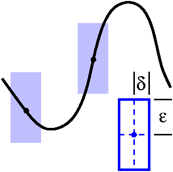
We can fix this with a smaller choice of the horizontal dimension, operating in the domain space. In this green box picture, that smaller choice allows the green shadow box, centered on a point on the previously troublesome steep part of the curve, to hold the curve inside and have it escape the vertical sides. Uniform continuity asserts that given a vertical dimension, there is some horizontal dimension so that if a congruent box is centered at each point of the curve, the part of the curve which is contained in the box will escape through the vertical sides.
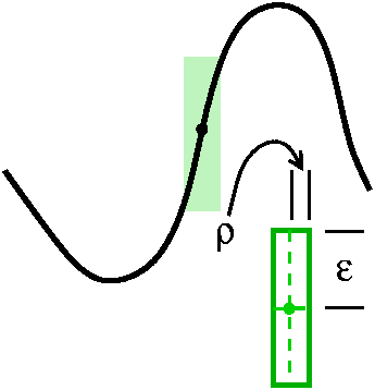A function satisfies a uniform Lipschitz condition if there is K>0 so that |f(x1)-f(x2|<=K|x1-x2|. The graph drawn is fairly smooth, and is presumably C1. If such a function also has a bounded derivative, then the function satisfies a uniform Lipschitz condition (this is implied by the Mean Value Theorem). This is more delicate, and indicates that a butterfly (!!) centered at each point of the graph would enclose the graph within its wings. Butterflies can be put into boxes, so functions satisfying uniform Lipschitz conditions are uniformly continuous. But boxes can't be put inside butterflies. More comprehensibly, sqrt(x) is uniformly continuous on [0,1] since it is continuous on a compact set. But it does not satisfy a Lipschitz condition at 0: Take x1 to be 0 in |f(x1)-f(x2|<=K|x1-x2| and get sqrt(x2)<=Kx2 for all x2>0. This means 1<=Ksqrt(x2) for such x2's (such as 1/{2K}), which is false for any K. Square root has no butterflies at 0.

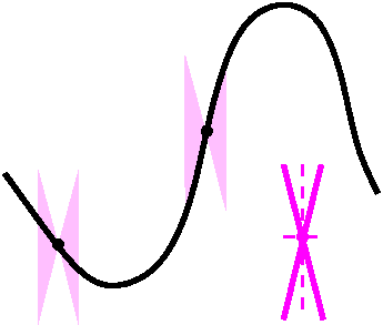END OF DIGRESSION

Suppose s is a continuous function from [a,b] to an open set U in C.
Claim There exists a partition of [a,b]: a=t₀<t₁<...<t_n-1<t_n=b and open discs D_rj(z_j) in U for 1<=j<=n such that for any j in {1,2,...,n}, s([_j-1,t_j]) is contained in D_rj(z_j).

Proof Let K=s([a,b]). U is open, so for k in K, there exists e_k such that D_ek(k) is in U. Therefore {D_ek(k)|k in K} is an open cover of K. Since the continuous image of a compact set is compact, K is compact. Therefore, there exists a Lebesgue number r for our open cover. f is uniformly continuous. So there exists a d>0 such that if [s₁,s₂] is in [a,b] and s₂-s₁ We can take an antiderivative F_j in each D_rj(z_j). This proof will be finished in the next class period.I hope.

Last class, we assumed that g=f´/f is C¹ so as to find an anti-derivative for g. However, we assumed that f was only C¹, which implies that g is C⁰. We cannot guarantee g has an antiderivative in this case. Professor Greenfield assured the class that g was in fact C¹ and that this result would be proved in two weeks.
But can we trust Professor Greenfield? Perhaps he will deceive us with a wrong use of the Axiom of Choice ...

We defined _a^b f(t) dt = _a^b g(t) dt + i _a^b h(t) dt where f:[a,b]--> C is continuous and f(t) = g(t) + i h(t). We then proved the following proposition.

Proposition: |_a^b f(t) dt|<=_a^b|f(t)|dt

Proof: If the integral is 0, the result is correct. Define h = [_a^b f(t) dt)/|_a^b f(t) dt|]. Observe that h is in C and |h|=1. We now perform the following sneaky calculation:
|_a^b f(t) dt|= h^-1_a^b f(t) dt = _a^b h^-1 f(t) dt = Re _a^b h^-1 f(t) dt = _a^b Re( h^-1 f(t) ) dt. Since Re(w)<=|w| for all w in C we conclude that |_a^b f(t) dt| =_a^b Re( h^-1 f(t) ) dt <=_a^b|h^-1 f(t)| dt = _a^b|f(t)|dt.

We then defined some terms. We said that s:[a,b]-->C is a C¹ curve if s(t) =s₁(t) + i s₂(t) and s₁, s₂ are C¹. Next we defined _sf(z)dz=_a^bf(s(t))s´(t)dt where f is continuous in an open subset U of C and s is a C¹ curve with s([a,b]) contained in U.

With these definitions we proved the following theorem:
Theorem 1: If F is holomorphic in U, F´=f, and s is a C¹ curve in U then _s f(z) dz = F(s(b))-F(s(a)).
Proof: Notice _s f(z)dz = _a^b f(s(t))s´(t) dt = _a^b F´(s(t))s&180;(t) dt = _a^b d/dt(F(s(t)) dt = F(s(b))-F(s(a)).

We also stated the following theorem. The proof is left as a homework problem since the instructor can't do it in public.

Theorem 2: (Reparameterization - Prop 2.1.9) Let s:[a,b]-->U be a C¹ curve, f continuous on U, and y:[c,d]-->[a,b] a one-to-one C¹ function with y(c)=a and y(d)=b. If t=s composed with y then _tf(z)dz = _sf(z)dz.

Theorem 2 shows that the parameterization of a curve doesn't matter when evaluating the integral.

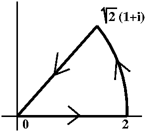EXAMPLE (I should have provided an example before going on!) Let's consider the closed curve shown, a line segment from 0 to 2, then a quarter circle for 1 to sqrt(2)(1+i), followed by a line segment from sqrt(2)(1+i) to 0. (Notice that |sqrt(2)(1+i)|=2.) I'll call this curve s. This is certainly a piecewise C¹ curve. I will just choose a polynomial of low degree in z and z-bar, since I am lazy. So suppose f(z)=1+2z+z(z-bar), a quadratic polynomial. Let's compute _sf(z)dz.
s is the sum (the concatenation!) of s₁+s₂+s₃, where s₁ and s₃ are line segments and s₂ is a circular arc.

1. Computing the integral over s₁: parameterize by just the function t, with t in [0,2]. Then the recipe _a^bf(s(t))s´(t)dt becomes:
       1+2z+z(z-bar)-->1+t+t²
       s´(t)dt-->dt
   and we compute ₀¹1+t+t²dt=t+(1/2)t²+(1/3)t³]₀¹=1+(1/2)+(1/3)=(11/6).
2. Computing the integral over s₂: parameterize by the function 2e^it, with t in [0,Pi/4]: this is a complex analysis course, and I will almost always parameterize circular arcs with exp! Then the recipe _a^bf(s(t))s´(t)dt becomes:
       1+2z+z(z-bar)-->1+4e^it+4
       s´(t)dt-->i2e^itdt
   and we compute ₀^Pi/4(1+4e^it+4)i2e^itdt ₀^Pi/42ie^it+8ie^2it+8ie^itdt =2e^it+4e^2it+8e^it]₀^Pi/4= ((2(1+i)/sqrt(2))+4i+8(1+i)/sqrt(2)(- (2+4+8)=5sqrt(2)(1+i)+4i-14.
3. Computing the integral over s₃: well, the line segment will be t-->e^iPi/4t for t in [0,2], but I need to reverse it, because the end of the segment should be the origin. So I must put in an additional -.     1+2z+z(z-bar)-->1+2e^iPi/4t+4t²
       s´(t)dt-->e^iPi/4dt
   Now compute -₀²(1+2e^iPi/4t+4t²)e^iPi/4dt. This is -e^iPi/4(t+e^iPi/4t²+(4/3)t³)]₀². Wow! There's nothing at 0, and the value at the top is -e^iPi/4(2+e^iPi/4+(32/3)) which is -sqrt(2)(1+i)-i-(16sqrt(2))/3.

Next we defined concatenation of curves. Suppose s:[a,b]-->C and t:[c,d]-->C are C⁰ s(b)=t(c). We then define (s+t)(t)=s(t) if a<=t<=b and s+t(t) = t(t-b+c) if b<=t<=b+d-c. So s+t is a curve whose domain is [a,b+d-c], We say that a curve is piecewise C¹ if it the finite sum of C¹ curves.

Next we made a provisional definition for the integral over a piecewise C¹ curve. If s=s₁+...+s_n where s_j is C¹ for 1<=j<=n then we define _sf(z)dz to be _s1f(z)dz+...+_snf(z)dz. The difficulty with this definition is that s may be expressed as two different sums of C¹ curves. For instance, we may have s=s₁+s₂ and s=t₁+t₂ with no simple relationship between the pieces individually. In order for our definition of the integral to make sense need the following Lemma.

Lemma: If s=s₁+..+s_n and s=t₁+..+t_m then _s1f(z)dz+...+_snf(z)dz is equal to _t1f(z)dz+...+_tmf(z)dz.
Proof Idea: This proof uses partitions from Calculus 1. Observe that it is possible to find a partition a=t₀<t₁<...<t_n=b so that s|_[tj-1,tj] = s_j. Likewise, there is a partition a=t^*₀<t^*₁<...<t^*_m=b so that s|_[t^*k1,t^*k]=t_k. One needs only to take the refinement of these partitions to see that the Lemma is true. And the refinement can be done by just adding one point to a given partition and proving equality of the resulting sum of integrals. Then both of the partitions given have a common refinement, obtained by taking their union. This common refinement can be gotten by including one more point a finite number of tiems.

After proving this lemma we discussed whether the prior theorems would also hold for piecewise curves. The first theorem holds due to the fact that the integral of a piecewise curve is a telescoping sum. The second theorem might be true. (Think about piecewise C¹ change of parameters.) We also defined -s:[a,b]--.C to be (-s)(t)=s(b+a-t) for s:[a,b]-->C, a C⁰ curve. We noted that _-sf(z)dz=-_s f(z)dz if f is C⁰ and s is piecewise C¹.

A C⁰ curve is closed if its start is the same as its end: s:[a,b]-->C with s(a)=s(b).

We discussed what it meant for two closed C⁰ curves s:[0,1]-->C and t:[0,1]-->C to be homotopic. We say that s is homotopic to t in U, written as s~t in U if there is a C⁰ mapping H:[0,1]x[0,1]-->U so that:

1. H(0,t)=s(t) for t in [0,1].
2. H(1,t)=t(t) for t in [0,1].
3. H(s,0)=H(s,1) for all s in [0,1].

We need the third requirement in the definition, otherwise detecting holes in domains (connected open sets) will be impossible with homotopies. Look at the picture below, which is supposed to be "snapshots" (?) of a fake homotopy, without the third requirement. We have a nice, continuous closed curve surrounding a hole in the first, leftmost picture. We then continuously deform the curve, now no longer closed, so it moves into a point. Hey: all continuous curves can be deformed continuously into a point if we don't have the third requirement.

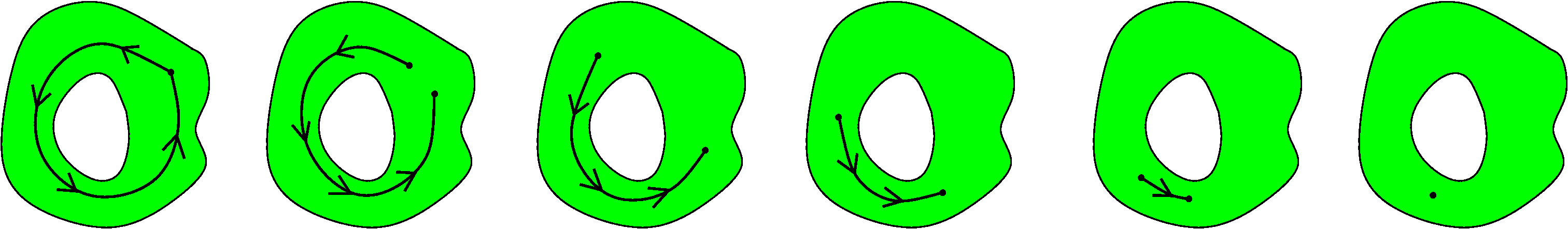
With this definition of homotopic we stated a version of Cauchy's Theorem.

Theorem: Suppose U is open in C. Suppose f is holomorphic on U. Suppose s and t are piecewise C¹ closed curves in U, and suppose s~t in U. Then _sf(z)dz=_tf(z)dz.

Since there is supposed to be a homotopy H(s,t) between t=H(0,t) and s=H(1,t), perhaps we should try to study the function s-->_{H(s,_)}f(z)dz. This is certainly natural. One technical problem is that we don't know how to define integration over the intermediate curves, H(s,_), which are only supposed to be continuous. In fact, I don't know how to define integration in general over these curves, but I can show you a way to define integration if the integrand, f, is assumed to be holomorphic.
I noted in class that the integration I was proposing to define would not allow us to compute length of an average continuous curve (!) because of this restriction on the integrand.

Next we began discussing how to define _sf(z)dz where s:[a,b]-->U is a C⁰ curve, U is open, and f:U-->C is holomorphic. Since the image of s is compact we are able to form a partition a=t₀<t₁<...<t_n=b so that the image of each interval [t_j-1,t_j] fits inside a disk D_j contained in U. Since there is F_j such that F_j´=f in D_j then we can define _s|[tj-1,tj]f(z)dz=F_j(s(t_j))-F_j(s(t_j-1)).

There are many details to check!

With the intent to prove Cauchy's Theorem we then proved the Lebesgue Number Lemma.

Lemma: Suppose K is a compact metric space and {U_a}_{a in A} is an open cover of K (this means each U_a is open and that the union of the U_a's is all of K). Then there exists a d>0 so that for all k in K, there exists a in A so that B_d(k)={x in K | d(x,k)<d} (the open ball of radius d and center k) is contained in U_a.
Proof: We use proof by contradiction. Suppose that the result is false. Then for all d>0, there is a k_d in K so that B_d(k_d) is not a subset of U_a, for all a in A. Well, to me, this is, if not the core of the proof, the principal pedagogical reason to present this particular proof: we should all be able to negate a complicated (?) three-layered quantified statement. Can you do such a negation?
We can then form a sequence {k_n} of K so that B_1/n(k_n) not a subset of U_a for all a in A. Since K is compact there is a subsequence {k_nj} that converges to a point k^* in K. But k^* must be in one of the U_a's, since we have an open cover of K.So there is a₀ in A with k^* in U_a0. Since U_a0 is open then there is e>0 such that B_e(k^*) is contained in U_a0. Since k_nj-->k^*, there is N>0 such that if j>= N then d(k_nj,k^*)<e/2. Recall that B_1/nj(k_nj) is not a subset of U_a, for all a in A. Thus B_1/nj(k_nj) is not a subset of U_a0. If we pick j₀>N with also 1/j₀<e/2 then we obtain a contradiction, for we have that B_1/n(j₀) is a subset of B_e(k^*) which is contained in U_a0. Use the triangle inequality.

The Wikipedia proof of this famous lemma is more direct, and avoids argument by contradiction which some people dislike. I think that proof resembles what Mr. Pal was suggesting, but I find the proof too elaborate, almost artificial. The Lebesgue number is a basic metric space topological idea, and I prefer proofs that I find simple.

Possibly relevant Latin quote and a possible translation:
De gustibus non est disputandum. There's no accounting for taste.

We started with a digression to fully understand the chain rule for complex functions. In R² calculus we find a horrible chain rule with matrices (Jacobian aka that matrix whose determinant is the Jacobian). Amazingly, simply manipulating the R² chain rule and understanding it in the context of complex functions (and utilizing the Cauchy-Riemann equations) turns it into the "regular" one for R: (fg)´ = f´(g)·g´ (complex multiplication). We like this very much.
Well, the Chain Rule in R² is a special case of, say, the Chain Rule in normed vector spaces. It is actually very nice. It states that the linear approximation to a composition is the composition of the linear approximations of the original functions. I disagree with the word, "horrible".

Back to our propositions -- During the last lesson, we proved propositions 1 and 2 using Poincaré's Lemma, but we didn't really appreciate the lemma enough because we didn't understand how much it would be difficult to prove these propositions without using it.

Before proving proposition 3, we give a definition: If V is an open set in C, then O(V) is the collection of holomorphic functions from V to C. So proposition 3 is now stated as: If U is the unit disc, and f in O(U) never vanishes then f has a logarithm in O(U) and this means there exists F in O(U) so that e^F=f. To amuse us all, the instructor gave us a corollary of this proposition: The unit group of O(U) is divisible. After some explanations, we were explained that "Algebra is a worthless swamp" Please delete. The instructor's mathematical taste is dubious.-- this corollary is just equivalent to saying that we can take roots (square, cube, ...) of non-vanishing holomorphic functions in the unit disc. We can prove this easily using proposition 3 by taking the logarithm, dividing, and plugging back into the exponential function [in the language of "Mathematics": f^(1/n) = e^((1/n) log f)].

Now we're ready to try proving the proposition. We first try without Poincaré's lemma:

"Proof 1"
We defined complex logarithms in an early (first?) lesson (but this is not in the diary notes...). Just compose the logarithm. This doesn't work because the logarithm is different for different areas of C\{0} and there is no simple way to patch them up to create one logarithm for the whole function (this is actually the covering homotopy property we all love from algebraic topology. It's quite difficult to prove it over "there", and it's just as difficult "here").

"Proof 2"
Take the power series for log. Of course, this proof has the exact same flaw as the previous one. You can't create one power series for log that covers "enough" of C\{0}.

Our Proof
If e^F=f then F´ should be f´/f. Define g=f´/f. Then g is in O(U) (here we use the fact that f is non-vanishing). By proposition 2 (which is proven using Poincaré's lemma) there is an anti-derivative to g. Let G be this anti-derivative. All that is left is to find the right constant to add to G, which is done easily. Wow, that was so simple and nice.

We now move on to understanding what integrals over closed curves are in C. We start with a small example motivated by our previous discussion (last lesson) about finding the anti-derivative of a holomorphic function -- if f is in O(U) then any integral on a rectangle of f is equal to 0. We prove this using Green's theorem and the Cauchy-Riemann equations. But what if U is not the unit circle? Then this is sometimes true and sometimes not. This is a very large and interesting issue and we will understand it better as the course progresses. But we should first define what a curve is. Old-fashioned people (like Ahlfors and Hille, our instructor's great-great-grandfather) define rectifiable continuous curves, which are not fun to work with. Well, many people would disagree with the "not fun" phrase. They would assert that such curves are actually the correct collection! Fortunately for us, our instructor is nice enough to allow us to work with piecewise C¹ curves. We are relieved.

I mentioned the effort to develop "complex analysis" without line integrals. Here is a reference: Topological analysis by G. T. Whyburn. QA611.W497 1964

We finished off with a brief description of Cauchy's theorem: Let D be a connected open set and f in O(D). Let Gamma be a piecewise C^1 closed curve which is homotopic to a point (we will discuss this in the next lesson) then the integral of f over Gamma is 0.

We thanked the instructor and left class happily.

The instructor mentioned his professional ancestors.

We then discussed the Poincaré Lemma. Well, Google has more than 900,000 links for this topic. Our version is a key local observation in the differential calculs of R². In the open unit disc with f and g C¹ in the disc, there is F with F_x=f and F_y=g when f_x=g_y (the "compatibility condition" for this overdetermined system of linear partial differential equations). The proof used the Fundamental Theorem of Calculus and differentiation under the integral.

How unique is such an F? This led to brief mention of connectedness, pathwise or arc connectedness, and connectedness using just concatenated horizontal and vertical line segments. F is unique up to an additive constant.

Then the instructor attempted (started?) to verify the following three corollaries of the Key Local Observation:

1. Every harmonic function in the disc has a harmonic conjugate. Well, we needed to define "harmonic function": h so that h_xx+h_yy=0. Occuring in heat distribution as a model of steady-state heat distribution on a thin homogeneous metal plate. We briefly considered harmonic polynomials. If u+i v is holomorphic with u and v being C² (it will turn out that the number of derivatives doesn't matter!) then both u and v are harmonic (a consequence of the CR equations). v is called a "harmonic conjugate" of u (but -u is a harmonic conjugate of v, sigh). We did prove this. There are harmonic functions in the punctured plane (all of C except the origin) which don't have harmonic conjugates.
2. Every holomorphic function in the disc has an antiderivative. A homework problem gives an example of a domain and a holomorphic function which doesn't have an antiderivative in the domain. A bit more needs to be said about this.
3. Every non-vanishing holomorphic function in the disc has a logarithm. This must be investigated.

I stated the Loomen-Menchoff Theorem: if the x and y derivatives of u and v all exist in some open set, and if these derivatives satisfy the CR equations, then u+iv is holomorphic. The proof of this relies on delicate measure-theoretic arguments, and the best reference I have is 6 pages in Narasimhan's book (see the text references, please).

Since both d/dz and d/dz-bar are pure first order PDE's, the sum, product, quotient (where defined), and composition of holomorphic functions is holomorphic, and the formulas for the derivatives are the familiar ones.

Then we discussed Euler's formula. For that we needed to digress and define the exponential function, which I did according to the text. I also stated this was the only reasonable definition. Here's a fact: there is a unique solution to the following PDE problem:
u and v are C¹ in C, they satisfy the CR equations in C, and u(x,0)=e^x (the calculus exponential) and v(x,0)=0. This is not totally obvious. The text supplies one solution but why couldn't there be others?

The text's solution to what is e^z is a homomorphism of the additive group of C to the multiplicative group of C. We also obtained formulas for the inverse, maybe called log. This function has some problems. First, exp is 2Pii periodic, so there are many logs. Second, I described how to define log explicitly in the right half-plane (there are similar formulas in the left and upper and lower half-planes). But there is no valid formula in all of C\{0}. What is arg? This log is holomorphic, and its derivative (we checked this in the right half-plane) is 1/z.

We very briefly discussed the group of roots of unity, an interesting group, and how it looks sitting in the unit circle |z|=1.

Then we finally proved: if z_j-->z then |z_j|-->|z|. We did this by proving the Lipschitz estimate mentioned last time, and then couldn't prove the triangle inequality efficiently. (Hint: someone should have suggested the Cauchy-Schwarz inequality.)

Mr. Pal mentioned the following proof for C: Re(z[conjugate w])<=|z[conjugate]w|=|z| |[conjugate]w|=|z| |w|.

Finally we began the first lecture of the course. I gave Kronecker's famous quote:
      God created the integers, all else is the work of man.
So we went from the positive integers to the integers to the rationals. Then briefly I remarked there were many choices of absolute values on the rationals, and that the "standard" one was rather exceptional. The rationals can be completed in any of these. We will choose the real numbers and neglect the p-adics. The real numbers are ordered, giving rise to other ways of understanding completeness (logicians are interested in wonderfully huge ordered fields!). So now we have the complete ordered field, R. Some of its finite dimensional vector spaces have interesting algebraic structure.

R² is a field, C, which can't be given a consistent structure of an ordered field (easy to prove). C also turns out to be the algebraic closure of R.

R⁴ is the quaternions (now we give up commutativity: this is a skew field, and has some neat subgroups). R⁸ is the octonions or Cayley numbers (now we give up associativity as well as commutativity, but this is a division algebra). I think there is also something interesting still about R¹⁶ but here's a reference with a more complete discussion:

Numbers by Heinz-Dieter Ebbinghaus (Author), Hans Hermes (Author), Friedrich Hirzebruch (Author), Max Koecher (Author), Klaus Mainzer (Author), JN|rgen Neukirch (Author), Alexander Prestel (Author), Reinhold Remmert (Author), John H. Ewing (Editor), K. Lamotke (Introduction), H.L.S. Orde (Translator)
in the library at QA241.Z3413 1990.

#9
This problem defined a specific function: i({1-z}/{1+z}), an example of a linear fractional transformation. It declared that the mapping established a bijective correspondance between the interior of the unit circle ("the unit disc") and those complex numbers with positive real part ("the upper halfplane"). The problem was solved by direct computation.
Why do this problem?
The problem introduced people to a sort of non-Euclidean view of geometry. We considered stereographic projection, establishing a correspondance between points in the plane and all points of the unit sphere in R³ except the North Pole. It turned out to be convenient to label this exceptional point , because then the correspondance provided a concrete representation of the 1-point compactification of the plane. It is also one-dimensional complex projective space, as we shall discuss. Under stereographic projection, the unit disc corresponds to the lower hemisphere, and the upper halfplane corresponds to the rear (?) hemisphere. The specific transformation just turns out to be a description of a rotation of the unit sphere turning one hemisphere into another. Each of the domains (unit disc, upper halfplane) is a natural place to explore hyperbolic geometry. The upper halfplane setting allows a natural group of transitive automorphisms to operate obviously (translations by real numbers and multiplications by positive real numbers). The unit disc model allows the stabilizer of a point, say the origin, to be described simply: just the rotations. We will need to verify these things in detail, of course. All the mappings involved are conformal: they preserve angles defined when C¹ paths intersect in the domain and are transformed to the range.

#31
This problem considered "pure" first-order partial differential operators in x and y. There is a unique pair, {partial/z} and {partial/z-bar}, which operate well on the functions z and z-bar in C.
Why do this problem?
The text defines holomorphic function to be a C¹ function which is annihilated by {partial/z-bar}. Consideration of this strange definition (one of many logically equivalent statements) led immediately to the Cauchy-Riemann equations. But why should these equations be important? We verified that if f(z)=f(x+iy)=u(x,y)+iv(x,y) has C¹ components and if f(z) is complex differentiable, then the Cauchy-Riemann equations are satisfied. We began to investigate some sort of converse statement were true. Some versions are, and we began to prove them. With C¹ assumptions, proof of one statement is almost easy, using the Mean Value Theorem of one variable calculus. We didn't exactly finish the proof. Discussion will continue.
We also showed that the L¹ and L² norms are equivalent in R². That is, suppose (a,b)=a+ib is in the plane. Making |a|+|b| small will force sqrt(a²+b²) small, and conversely. This is true for any pair of norms in R² (or, indeed, in Rⁿ for n finite): not a totally obvious fact. We won't need the general fact, and will only verify if for pairs of norms we will encounter. Probably the only other example will be the L norm, which is max(|a|,|b|).

Here are other problems I requested, and why I thought they might be interesting:

#36
Write {partial/z} and {partial/z-bar} in polar coordinates.
Why do this problem?
This is not a very pretty computation, but sometimes we need to do dirty computations. The result might be useful, so let's see it.

#20 and #24
The first problem is a verification and use of Euler's formula. The second problem declares that the sum of the k^th (k>1) roots of a complex number must be 0.
Why do this problem?
Both of these problems need the introduction of some notion of the complex exponential function. So we can explore how the text introduces this function. We then could get Euler's formula, which has many uses. The second problem needs Euler's formula to establish the existence of k^th roots!

#23
Prove that |z| is continuous. The text suggests verifying that if z_j->z, then |z_j|->|z|.
Why do this problem?
Various irritating approaches can be made to this problem, but maybe the most satisfying method is to prove
||z|-|w||<=|z-w|
since this declares that |z| is a Lipschitz function and the limit statements are then clear. C¹ functions are locally Lipschitz, but |z| is certainly not C¹ in any neighborhood of 0.
Verification of the inequality needs work with the Triangle Inequality, so we would need to think about the Triangle Inequality. Distances from sets (here |z| measures the distance from 0) typically arise in a number of analytic problems, and the smoothness (or lack of smoothness!) is good to be acquainted with.

Maintained by greenfie@math.rutgers.edu and last modified 9/5/2007.
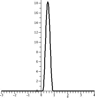
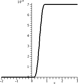
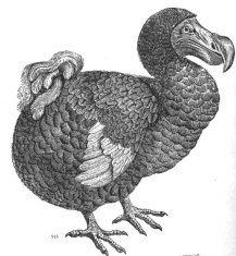