Significant example
I wanted to diagonalize
the matrix A given by
( 0 -1 1)
(-1  1 2)
( 1  2 1)
I will need (if possible, but it will be possible!) to find an invertible matrix C and a diagonal matrix D so that C-1AC=D. The diagonal entries in D will be the eigenvalues of A, in order, and the columns of C will be corresponding eigenvectors of A. the characteristic polynomial of C is
(-which I computed somehow and it was what I thought it would be. Maple has the following command:-1 1) det(-1 1-
>charpoly(A,x);
                          3      2
                         x  - 2 x  - 5 x + 6
I found one
eigenvector, and students, as their QotD, found the others.
If ![]() =1, take (2,-1,1)
=1, take (2,-1,1)
If ![]() =-2, take (-1,-1,1)
=-2, take (-1,-1,1)
If ![]() =3, take (0,1,1).
=3, take (0,1,1).
I asked students to look at these eigenvectors. They did, and we
didn't seem to learn much.
The C matrix is
( 2 -1 0)
(-1 -1 1)
( 1  1 1)
Now look at Ct:
( 2 -1 1)
(-1 -1 1)
( 0  1 1)
We computed the matrix product CtC. The result was
(6 0 0)
(0 3 0)
(0 0 2)
The 0's were caused by the orthogonality of the different vectors in the basis of eigenvectors. If the result had diagonal entries 1, 1, and 1, then the transpose would be the inverse. But I can make this happen by choosing slightly different eigenvectors: multiplying them by a scalar ("normalizing" them) to have length 1. So choose C to be, instead,
( 2/sqrt(6) -1/sqrt(3)    0     )
(-1/sqrt(6)  1/sqrt(3) 1/sqrt(2))
(-1/sqrt(6)  1/sqrt(3) 1/sqrt(2))
and then the transpose of C will be C-1. This really is remarkable.
The major result
We can always diagonalize any symmetric matrix by using a matrix of
normalized eigenvalues. The eigenvalues are orthogonal, and the
resulting matrix used for changing bases has the wonderful property
that its inverse is its transpose. A matrix C such that
C-1=Ct is called orthogonal.
Here's another version:
| Every symmetric matrix has a basis of orthogonal eigenvectors, which, when normalized, form an orthogonal matrix. The matrix of eigenvectors and its {inverse|transpose} diagonalize the symmetric matrix. |
This result is not easy to prove, and is usually the triumph (?) of our Math 250 course.
Why is an orthonormal basis (length of each basis element 1 and each perpendicular to the other) nice to compute with? Well, look:
The vectors v1=(3,1,2) and v2=(-1,3,2) and v3=(2,1,2) form a basis of R3. (You can check this by computing the determinant of the matrix obtained by sticking the vectors together to make a 3-by-3 matrix: the determinant is 4 and since this is not 0, the matrix has rank 3). This means that any vector in R3 can be written as a linear combination of v1, v2, and v3. Suppose the vector is (44,39,16). What is the linear combination? Uhhh ... with some effort, Maple and I came up with
(44,39,16)=(149/2)v1+(31/2)v2-82v2.
The vectors e1=(2/sqrt(6),-1/sqrt(6),-1/sqrt(6)) and e2=(-1/sqrt(3),1/sqrt(3),1/sqrt(3)) and e3=(0,1/sqrt(2),1/sqrt(2)) form an orthonormal basis. Now if I want to write
(44,39,16)=ae1+be2+ce3 just take the inner product with respect to e1 and use properties 1 and 2 of inner product above: <(44,39,16),e1>=a<e1,e1>+b<e2,e1>+c<e3,e1>=a. This is because <ei,ej> equals 0 if i is different from j and equals 1 if they are the same.
Therefore a=<(44,39,16),(2/sqrt(6),-1/sqrt(6),-1/sqrt(6))>=(44·2-39-16)/sqrt(6), similarly, b=<(44,39,16),e2> and c=<(44,39,16),e3>. It is very easy to find the coefficients in the linear combination when we have linear combinations of orthonormal vectors.
Transition...
It turns out that this way of looking at symmetric matrices, using
orthogonal change of basis to get a diagonal matrix, was so successful
that it has been applied to many things, in particular to the study of
ordinary and partial differential equations. The setting might seem
initially somewhat strange to you, but as your understanding
increases, as I hope it will, you should see the analogy more
clearly.
HOMEWORK
Please read sections 8.8, 8.10, and 8.12 of the text. The following
problems almost surely can be done easily by Maple or
Matlab or any grown-up calculator. I strongly urge
students to do these problems by hand and get the correct
answers.
8.8: 13, 19.
8.10: 15
8.12: 17, 39.
|
Monday, October 31 |
|
Thanks to Ms. Rose for putting a
solution to the previous QotD on the board. That was the
following:
Find an eigenvector associated to the eigenvalue 2 for the matrix
(5 2)
(3 4)
So for this we need to solve
(5-2  2 )(x1) = (0)
( 3  4-2)(x2)   (0)
This system is just
3x1+2x2=0
3x1+2x2=0
and we need to find a non-trivial solution. Well, these are all multiples of (1,-3/2). I chose (2,-3) as my eigenvector in what follows.
Now what?
Well, we know that if A is the 2-by-2 matrix
(5 2)
(3 4)
then A has eigenvalue 2 with one associated eigenvector (2,-3) and
eigenvalue 7 with one associated eigenvector (1,1). This is neat.
Here is what you should consider.
Start with R2, and (thinking about
(x1,x2) as a column vector) multiply by A,
getting another vector in R2.
I have a basis of eigenvectors. Maybe I can rethink multiplication by A into three stages. Here I will start with a vector described in terms of the standard basis (1,0) and (0,1).
- Change information to be in terms of the basis of eigenvectors.
- Multiply by A.
- Change back to the standard basis information.
I want to change (1,0) as a column vector to (1,1) and change (0,1) as a column vector to (2,-3). So I need to find a matrix C (for change of basis) which does the following:
(a b)(1) is ( 2) and (a b)(0) is (1).
(c d)(0)    (-3)     (c d)(1)    (1)
This isn't too difficult: a and c are specified by the first requirement and b and d are specified by the second requirement. Therefore C=
( 2  1)
(-3 1)
How can I undo switching information from the standard basis to the basis of eigenvectors? "Clearly" I should find C-1:
( 2 1 | 1 0)~(1 1/2 | 1/2 0)~(1 0 | 1/5 -1/5 )
(-3 1 | 0 1) (0 5/2 | 3/2 1) (0 1 | 3/5  2/5 )
We checked that the result was indeed C-1.
A multiplication
I computed C-1AC. I noted that this could be computed in
two ways, as (C-1A)C or as
C-1(AC). Matrix multiplication is
associative so you can regroup as you wish. It is not
always commutative (recall an early linear
algebra QotD!) so you can't change the order of the matrices you
are multiplying.
      C-1 A                                                  C-1AC
(1/5 -1/5)(5 2) is ( 2/5 -2/5) and then ( 2/5 -2/5)( 2 1) is (2 0).
(3/5  2/5)(3 4)    (21/5 14/5)          (21/5 14/5)(-3 1)    (0 7)
I'll call the diagonal matrix just D. You should see, I hope, that this computation verifies the philosphy above. Finding an invertible matrix C and a diagonal matrix D so that C-1AC=D is called diagonalization. We could also write A=CDC-1.
Why do this?
Computations with diagonal matrics are very easy. For example,
D2 is just
(22 0)
(0 72)
In fact, D10 is
(210 0)
(0 710)
Now A10=A·A····A (ten times).
But since A=CDC-1, I know that A10=CDC-1·CDC-1····CDC-1. Now we can associate in any way: put parentheses around the factors of the product. The C-1C on the "inside" cancel each other. So A10=CD(C-1·C)D(C-1····C)DC-1=CD10C-1. So we can find powers of A by finding powers of the diagonal matrix.
Computational "load"
There's an initial computation needed to find the eigenvalues and
eigenvectors (that's C and D) and then C-1. But once that
is done, then finding powers of A is much faster. And even finding
exponentials of A is faster.
eA=SUMn=0infinity(1/n!)An=SUMn=0infinity(1/n!)CDnC-1.
Now Dn is
(2n 0)
(0 7n)
and SUMn=0infinity(1/n!)CDnC-1=C(SUMn=0infinity(1/n!)Dn)C-1. What is SUMn=0infinity(1/n!)Dn? It is
(SUMn=0infinity2n/n! 0)
(0 SUMn=0infinity7n/n!)
and this is eD=
(e2 0)
(0 e7)
So a potentially complicated sum, SUMn=0infinity(1/n!)An, is actually CeDC-1: a very simple computation.
Such a computation can help to write solutions of such systems as
(dx/dt}=5x(t)+2y(t)
{dy/dt}=3x(t)+4y(t)
If we make X(t) the column vector corresponding to (x(t),y(t)), then
this system can be abbreviated in matrix form as X'(t)=AX(t). By
analogy with the scalar case, I would hope that a solution could be
written as X(t)=eAt(Const), and here the (Const) would be a
2 by 1 column vector of initial conditions: x(0) and y(0).
I was going to compute another example. Let me show you what this would have been:
> with(linalg):
Warning, the protected names norm and trace have been redefined and unprotected
> A:=matrix(3,3,[1,2,2,-1,1,1,2-1,-1]); #Not a very random matrix.
#2nd col=3rd col, so rank is 2.
                                  [ 1     2     2]
                                  [              ]
                             A := [-1     1     1]
                                  [              ]
                                  [ 2    -1    -1]
> charpoly(A,x); #0 is an eigenvalue of A, and then with a common
#factor of x deleted, the result is a quadratic which can be factored.
                                  3    2
                                 x  - x  - 2 x
> eigenvects(A);#A list of eigenvalues and eigenvectors.
      [0, 1, {[0, -1, 1]}], [-1, 1, {[1, 2, -3]}], [2, 1, {[-4, 1, -3]}]
> C:=matrix(3,3,[0,1,-4,-1,2,1,1,-3,-3]); #Changing basis to the
#basis of eigenvectors.
                                  [ 0     1    -4]
                                  [              ]
                             C := [-1     2     1]
                                  [              ]
                                  [ 1    -3    -3]
> inverse(C);#Back from the eigenvectors to the "standard" basis.
                            [1/2     -5/2    -3/2]
                            [                    ]
                            [1/3     -2/3    -2/3]
                            [                    ]
                            [-1/6    -1/6    -1/6]
> evalm(inverse(C)&*A&*C);#Verifying that we've got a diagonalization.
                                [0     0    0]
                                [            ]
                                [0    -1    0]
                                [            ]
                                [0     0    2]
When can we diagonalize a matrix?
Certainly if we knew that Rn had a basis of eigenvectors of
A, then we can diagonalize A. We'd just assemble C by filling in the
eigenvectors as columns of C. And D would be a diagonal matrix with
diagonal entries the eigenvalues of A in the same order as the matrix
C was assembled. And C-1AC=D.
What problems could you expect?
 Consider the matrix A=
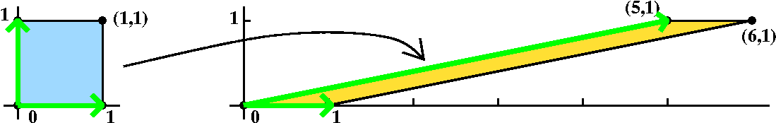
(1 5)
(0 1)
This matrix represents a shear. Its determinant is 1. The area magnification factor is 1. The picture shows what happens to the unit square under multiplication by A. det(A-
(1-1  5 )(x1)=(0)
( 0  1-1)(x2) (0)
so 5x2=0. Therefore x2 must be 0. The eigenvectors are all (non-zero!) multiples of (1,0).
There are not enough eigenvectors to be a basis of R2.
Now look at A=
( 1/sqrt(2) -1/sqrt(2) )
( 1/sqrt(2)  1/sqrt(2) )
This takes (1,0) to the vector (1/sqrt(2),1/sqrt(2)) and the vector (0,1) to (-1/sqrt(2),1/sqrt(2)). It is rotation by Pi/4 (45o) around the origin. The determinant is again 1, so there is no area distortion. det(A-
There are no real eigenvalues.
So you would need to compute using complex numbers to diagonalize this matrix (in C2, not R2!).
Some realistic conditions
The matrices occuring in engineering applications are rarely
"random". They frequently have some internal structure. The simplest
structures to explain are symmetric and skew-symmetric.
A matrix is symmetric if it is equal to its transpose.
Such a matrix must be square, otherwise its dimensions could not
agree. An example is, say, in a molecule, if the (i,j)th
entry is the distance between atom i and atom j. Then since distance
is symmetric, so is the matrix. On a road map, frequently you will
find that the printer uses storage efficiently by only printing half
of the table containing distances between cities. Symmetry permits
storage to be halved!
Examples
( 5 3)  ( 7 1  4)
(-3 2)  (-1 2 -6)
        (-4 6 -3)
A matrix is skew-symmetric if it is equal to minus its
transpose.
Again, such a matrix must be square, otherwise its dimensions could not
agree. An example is, say, in a molecule, if the (i,j)th
entry is the force from atom i to atom j. The force is a directed
quantity, so the (i,j)th entry is minus the
(j,i)th entry.
Also skewsymmetry permits
storage to be halved!
Examples
( 0 3)  ( 0 1  4)
(-3 0)  (-1 0 -6)
        (-4 6  0)
Please notice that the diagonal entries of a skew-symmetric matrix are
always 0. The determinant of the first example is 9, and the
determinant of the second example is 0. Indeed (!) the determinant of
an n-by-n skewsymmetric matrix is positive if n is even and is 0 if n
is odd. This is because det(A)=det(At) as we already
observed,
and det(-A)=(-1)ndet(A).
I then recalled the {dot|scalar|inner} product for vectors in Rn. If x=(x1,x2,...,xn) y=(y1,y2,...,yn) then <x,y>=SUMj=1nxjyj. In matrix form this is xty, converting the "row vector" x to a "column vector" and then multiply as matrices to get a number.
If A is an n-by-n matrix, we've studied the geometric effect of multiplying vectors x by A. Actually, that's really the matrix multiplication Axt, and then another transpose to get the darn column vector back to a row vector: (Axt)t.
I then tried to verify that <Ax,y>=<x,Aty>.
This has an immediate consequence that eigenvectors corresponding to distinct eigenvectors of a symmetric matrix are orthogonal. More to come!
|
Thursday, October 27 |
|
What did I do? I wrote a "random" 3-by-3 matrix (yeah, yeah, with small integer entries!), and then proceeded to check the textbook's formula for A-1. The formula I refer to is on p. 383 (Theorem 8.18). I believe engineering students should be aware that such an explicit formula exists, so that if such a formula is necessary, then it can be used.
I had students compute the entries of the adjoint of A, and we checked (at least a little bit!) that the result was A-1. I decided for the purposes of this diary to have Maple find minors, then get determinants, then adjust the signs, and then take the transpose: the result should be (after division of the entries by det(A)) the inverse. And it was. I mention that it took me longer to write the darn Maple code than it did to have people do the computations in class. The # indicates a comment in Maple and is ignored by the program.
> with(linalg):
Warning, the protected names norm and trace have been redefined and unprotected
> A:=matrix(3,3,[1,-2,3,2,1,0,2,1,3]); #defines a matrix, A.
                                   [1    -2    3]
                                   [            ]
                              A := [2     1    0]
                                   [            ]
                                   [2     1    3]

> det(A); #Finds the determinant
                                      15

> minor(A,2,1);  #This gets the (2,1) minor, apparently.
                                   [-2    3]
                                   [       ]
                                   [ 1    3]

>B:=matrix(3,3,[seq(seq((-1)^(i+j)*det(minor(A,i,j)),j=1..3),i=1..3)]);
#This mess, when parsed correctly, creates almost the adjoint of A.
                                  [ 3    -6     0]
                                  [              ]
                             B := [ 9    -3    -5]
                                  [              ]
                                  [-3     6     5]
> evalm(A&*transpose(B)); #We need to divide by 15, which is det(A).
# evalm and &* do matrix multiplication.
                               [15     0     0]
                               [              ]
                               [ 0    15     0]
                               [              ]
                               [ 0     0    15]

> inverse(A);
                            [1/5     3/5     -1/5]
                            [                    ]
                            [-2/5    -1/5    2/5 ]
                            [                    ]
                            [ 0      -1/3    1/3 ]

> evalm((1/15)*transpose(B)); # I think Bt is the adjoint of A.
                            [1/5     3/5     -1/5]
                            [                    ]
                            [-2/5    -1/5    2/5 ]
                            [                    ]
                            [ 0      -1/3    1/3 ]
> Y:=matrix(3,1,[y1,y2,y3]);
                                        [y1]
                                        [  ]
                                   B := [y2]
                                        [  ]
                                        [y3]

> evalm(inverse(A)&*Y); # How to solve the matrix equation AX=Y
# Left multiply by A-1.
                            [  y1    3 y2    y3  ]
                            [ ---- + ---- - ---- ]
                            [  5      5      5   ]
                            [                    ]
                            [  2 y1    y2    2 y3]
                            [- ---- - ---- + ----]
                            [   5      5      5  ]
                            [                    ]
                            [      y2     y3     ]
                            [   - ---- + ----    ]
                            [      3      3      ]

> A2:=matrix(3,3,[1,y1,3,2,y2,0,2,y3,3]); # Preparing for Cramer's rule
                                   [1    y1    3]
                                   [            ]
                             A2 := [2    y2    0]
                                   [            ]
                                   [2    y3    3]

> det(A2)/det(A); # The same result as the second entry in A-1.
                               2 y1    y2    2 y3
                             - ---- - ---- + ----
                                5      5      5
I "verified" Cramer's rule in a specific case. A similar computation
is shown above done by Maple. Thie is on p. 392, Theorem
8.23, of the text.
I have never used Cramer's rule in any significant situation. But, again, if you need such an explicit formula, you should be aware that it exists. But I also mention that, using my Maple on a fairly new computer, over half a second was needed to computing the inverse of a 5-by-5 symbolic matrix took half a second. So you should recognize the time/space requirements for such computations. Sigh.
This is all too many formulas, especially since they are not likely to be used. Mr. Pappas asked how they might be used in the real world, and my reply was that the matrices which students were likely to work with probably would have some structure: they might be sparse, with, say, entries non-zero only on or near the diagonal (spline algorithms), or they might have some perceptible block structure. For these matrices, running time frequently can be trimmed quite a bit. But still there will be problems in implementation (numerical stability) and writing and using programs needs some care.
Something a bit different
I've neglected to discuss the geometrical effect of a matrix. My model
matrix here will be 2-by-2, just A=
( 5 2 )
( 3 4 )
Geometry: det as area distortion factor
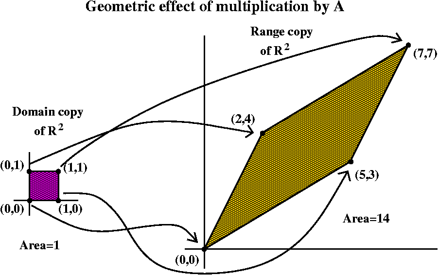 det(A), which is in this case 20-6=14, represents the area distortion
factor as A maps R2 to R2. That is, take
X=(x1,x2), and feed it into A. By this I mean do
the following: take the transpose, multiply by A, and then look at the
point you get in R2 (I guess another transpose is
needed). So the output is, I hope,
(5x1+2x2,3x1+4x2).
You can compute that:
det(A), which is in this case 20-6=14, represents the area distortion
factor as A maps R2 to R2. That is, take
X=(x1,x2), and feed it into A. By this I mean do
the following: take the transpose, multiply by A, and then look at the
point you get in R2 (I guess another transpose is
needed). So the output is, I hope,
(5x1+2x2,3x1+4x2).
You can compute that:- (0,0) gets changed to (0,0).
- (1,0) gets changed to (5,3).
- (0,1) gets changed to (2,4).
- (1,1) gets changed to (7,7).
The image of the unit square is a parellelogram, and the area is 14. All areas are determined by multiples and movements of the unit square (think about it: you fill things up with tiny little squares, etc.) so all affected areas are multiplied by 14.
One nice consequence is the following:
If A and B are n-by-n matrices, then det(AB)=det(A)det(B).
Comment Since A "maps" Rn to Rn by
matrix multiplication, and det(A), it turns out, is the way
n-dimensional volumes are stretched. So multiplying by A and then by B
concatenates the effects. N
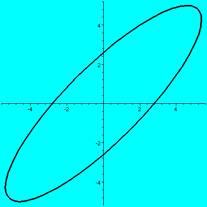
Geometry: the circle transformed by a matrix
Now here is what I showed on the screen as I attempted to catch up
with the last decade or so of the twentieth century in terms of
technical pedagogy.
>A:=matrix(2,2,[5,2,3,4]);
                                 [5    2]
                            A := [      ]
                                 [3    4]

>plot([5*cos(t)+2*sin(t),3*cos(t)+4*sin(t),t=0..2*Pi],
thickness=3,color=black);
|
|
>B:=evalm(A^2);
                                [31    18]
                           B := [        ]
                                [27    22]

>plot([31*cos(t)+18*sin(t),27*cos(t)+22*sin(t),t=0..2*Pi],
thickness=3,color=black);
|
|
>eigenvects(A);
                [2, 1, {[1, -3/2]}], [7, 1, {[1, 1]}]
 So we are looking at the effect of the matrix on the unit
circle, those points (x,y) in the plane which can be written as
(cos(t),sin(t)) for t between 0 and 2Pi. This is a circle. Then a
matrix, A, creates what is called a linear transformation,
which is a mapping taking R2 to R2 and taking
linear combinations in the domain to corresponding linear combinations
in the range.
So we are looking at the effect of the matrix on the unit
circle, those points (x,y) in the plane which can be written as
(cos(t),sin(t)) for t between 0 and 2Pi. This is a circle. Then a
matrix, A, creates what is called a linear transformation,
which is a mapping taking R2 to R2 and taking
linear combinations in the domain to corresponding linear combinations
in the range.
If A=
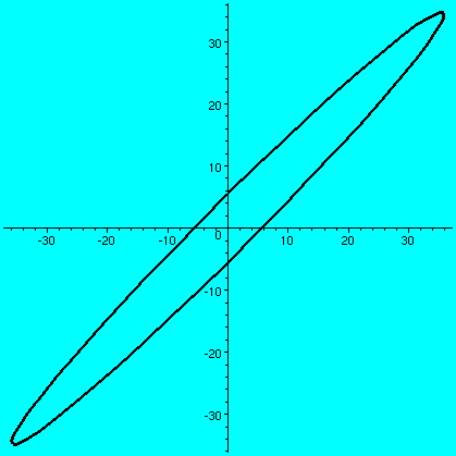
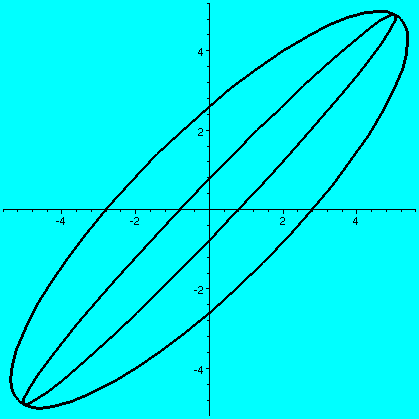
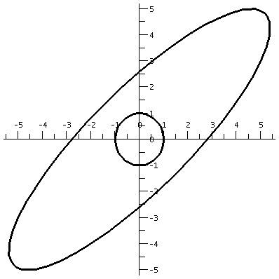
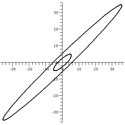
(a b)
(c d)
and if a vector X in R2 is (x1,x2), then AXt (the transpose changes the row vector to a column vector) is (back in row vector form [another transpose]) the point (ax1+bx2,cx1+dx2). What does this look like geometrically? The circle gets distorted geometrically. It turns out that for many matrices, the figure obtained will be an ellipse, with (0,0) as center of symmetry. The biggest stretch of this ellipse is in a certain direction. If we then multiply again by A, (that's B in this case, the evalm command in Maple asks it to do arithmetic on matrices) the picture is another matrix. Because the pictures are a bit difficult to compare, I asked Maple to rescale (important!) and graph both pictures together. The B picture is the narrower one, inside the A picture's ellipse. One way to find this principal preferred direction, where A seems to want to send stuff, is (as I tried to suggest in class) to take a point on the circle at random. Then some high power of A will likely send it more or less in about the correct direction (!!). This direction is called an eigenvector.
 |
 |
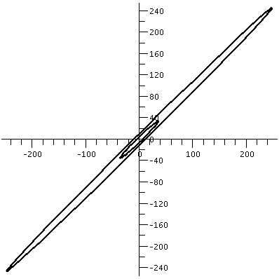 |
| The unit circle and its transform by A. The graph goes from about -5.5 to 5.5 both horizontally and vertically. | The transform by A and by A2. The graph goes from about -35 to 35 both horizontally and vertically. | The transform by A2 and by A3. The graph goes from about -245 to 245 both horizontally and vertically. |
Eigenvectors, eigenvalues, etc.
|
|
Understanding eigenvalues and eigenvectors is important if you are
going to any sort of extensive computation with matrices (by hand, by
computer, by thinking). As I observed in class, the requirement that
an eigenvector be not equal to 0 is very important. Without it,
any value ![]() is an eigenvalue! Eigen{value|vector} is also called
characteristic {value|vector} and proper {value|vector}, depending on
what you read and what you work with.
is an eigenvalue! Eigen{value|vector} is also called
characteristic {value|vector} and proper {value|vector}, depending on
what you read and what you work with.
Example
I worked out the details, the indispensable details, of course,
for the example which generated the pictures above. So A=
(5 2)
(3 4)
and if X is (x1,x2) then we would like to find solutions of the system corresponding to the matrix equation AXt=
5x1+2x2=and this sytem is the same as
(5-I want non-trivial solutions to this homogeneous system. This is the same as asking that the RREF of the system's coefficient matrix is not equal to I2, the 2-by-2 identity matrix. And this is the same as asking that the system's coefficient matrix be singular. We can test for singularity by asking for which
(5-has determinant 0. It is easy to find the determinant of this matrix: it is (5-
|
|
The roots of ![]() 2-9
2-9![]() +14=0 are 7 and 2. Nice people could
factor this polynomial, which will work since it is an example in a
classroom. People who wear suspenders and a belt on their
pajamas use the quadratic formula. By the way, there is no general
formula for the roots of a polynomial, and frequently numerical
approximation schemes are needed. Knowing these values of
+14=0 are 7 and 2. Nice people could
factor this polynomial, which will work since it is an example in a
classroom. People who wear suspenders and a belt on their
pajamas use the quadratic formula. By the way, there is no general
formula for the roots of a polynomial, and frequently numerical
approximation schemes are needed. Knowing these values of ![]() doesn't end our task. I would like
to find eigenvectors for each of these eigenvalues.
doesn't end our task. I would like
to find eigenvectors for each of these eigenvalues.
![]() =7
=7
Go back to the homogeneous system
(5-and plug in
-2x1+2x2=0
3x1-3x2=0
and the equations are a multiple of one another, so solutions are what solves x1-x2=0. One solution is (1,1). Another is (-46,-46). Etc.
QotD
Find an eigenvector associated to the eigenvalue 2.
HOMEWORK
We'll be
ending the official linear algebra part of the course this coming
week. You should try to read the remainder of the part of chapter 8
which we
will cover.
Please hand in these problems on Monday: 8.5: 33, 37, 39, 8.8: 6, 21.
|
Monday, October 24 |
|
Mr. Naumann kindly put the answer to the previous QotD on the board. It is necessary to know a bit about determinants to get the correct sign. Your "feelings" based on 2-by-2 and 3-by-3 determinant experience won't always be correct.
The last homework problem assigned (8.6: 58) was probably the most realistic we'll have this whole semester. The idea is to "approximate" the solution of a partial differential equation (to be discussed later in the course). The matrix involved
(-4  1  0  1 )
( 1 -4  1  0 )
( 0  1 -4  1 )
( 1  0  1 -4 )
should really be seen as an example of a much larger matrix, with lots of 0 entries and sort of "stripes" of 1's and -4's running diagonally. This is an example of what is called a sparse matrix (that term has almost two million Google entries!). An "average" (?) matrix might have n2 non-zero entries. A sparse matrix will have about (Constant)n non-zero entries. Computations with sparse matrices can frequently be done faster and more efficiently than with general matrices.
| I then remarked that my accumulation of |
| is being written partly because on the next exam I will ask for the definitions of linear algebra objects. Little partial credit will be given or can be earned with such questions: there's really only one way to answer questions about definitions. I therefore respectfully request that students be familiar with these definitions. |
So the stuff last time was really background. I don't think you need to know everything I discussed, but I do honestly believe that engineers should have some feeling for the real definition, even if it is very painful (and it is, indeed it is). Determinants come up constantly in complicated calculations. If you ever see big formulas involving addition of lots of choices of signs and products in applications, my guess is that some determinants will be hiding behind the curtains, and maybe if you recognize this you can understand the situation and the computations better.
If we look at the definition of determinant you
can see for every rook that's in the upper right-hand quadrant of
another rook, that other rook is in the lower left-hand quadrant of
the first rook. From this I hope you are willing to believe that the
determinant of a matrix is the same as the determinant of its
transpose. Ooops: I need to define transpose:
If B is a p-by-q matrix, then Bt, the transpose of
B, is a q-by-p matrix, and the (i,j)th entry of
Bt is the (j,i)th entry of B.
       ( 5 z 27 4 )            (  5  0  r )
If B = ( 0 k -1 2 ) then Bt is (  z  k  2 )
       ( r 2 .3 1 )            ( 27 -1 .3 )
                               (  4  2  1 )
Fact: If A is a square matrix, then det(A)=det(At)Another (and very useful!) consequence is that to determinant, rows and columns are "the same". Any determinant fact regarding rows has a corresponding fact regarding columns.
Row operations and determinants
We discussed how row operations change determinants. I tried to indicate
why the first and second of the following facts were true using
the definition of determinant which I gave, but I could not, considered
the time allocation and objectives of the course, tell why the last
fact is true.
| Row operations and their effects on determinants | ||
|---|---|---|
| The row operation | What it does to det | |
| Multiply a row by a constant | Multiplies det by that constant | |
| Interchange adjacent rows | Multiplies det by -1 | |
| Add a row to another row | Doesn't change det | |
Examples
Suppose A is this matrix:
( -3  4  0 18 )
(  2 -9  5  6 )
( 22 14 -3 -4 )
(  4  7 22  5 )
Then the following matrix has determinant twice the value of det(A):
( -6  8  0 36 )
(  2 -9  5  6 )
( 22 14 -3 -4 )
(  4  7 22  5 )
because the first row is doubled.
Also, the following matrix has determinant -det(A)
( -3  4  0 18 )
( 22 14 -3 -4 )
(  2 -9  5  6 )
(  4  7 22  5 )
because the second and third rows are interchanged. Notice that you've got to keep track of signs, so that if we interchange, say, the second and fourth rows leaves the value of the determinant would not be changed.
The following matrix has the same value of determinant as det(A)
( -3  4  0 18 )
(  2 -9  5  6 )
( 24  5  2  2 )
(  4  7 22  5 )
because I got it by adding the second row to the third row and placing the result in the third row.
Math 250 again
I also mentioned a beautiful (?) example of another exam problem from Math
250: suppose C is a 5-by-5 matrix, and det(C)=-7. What is det(2C)?
This takes a bit of thought, because we are actually multiplying each
of the 5 rows of C by 2. Therefore we multiply the determinant
by 2·2·2·2·2=25=32. So
det(2C)=(-7)·32=-224.
Silly examples (?)
Look:
   ( 1 2 3 )    ( 2 3 4 )
det( 4 5 6 )=det( 3 3 3 ) (row2-row1)
   ( 7 8 9 )    ( 3 3 3 ) (row3-row2)
Now if two rows are identical, the det is 0, since interchanging them both changes the sign and leaves the matrix unchanged. So since det(A)=-det(A), det(A) must be 0.
Look even more at this:
   (   1   4   9  16 )    (  1  4   9  16 )                (  1  4  9 16 )
det(  25  36  49  64 )=det( 24 32  40  48 ) (row2-row1)=det( 24 32 40 48 )
   (  81 100 121 144 )    ( 56 64  72  80 ) (row3-row2)    ( 32 32 32 32 ) (row3-row2)
   ( 169 196 225 256 )    ( 88 96 104 112 ) (row4-row3)    ( 32 32 32 32 ) (row3-row2)
so since the result has two identical rows, the deteminant of the original matrix must be 0.
There are all sorts of tricky things one can do with determinant evaluations, if you want. Please notice that the linear systems gotten from, say, the finite element method applied to important PDE's definitely give coefficient matrices which are not random: they have lots of structure. So the tricky things above aren't that ridiculous.
Use row operations to ...
One standard way of evaluating determinants is to use row operations
to change a matrix to either upper or lower triangular form (or even
diagonal form, if you are lucky). Then the determinant will be the
product of the diagonal terms. Here I used row operations (actually I
had Maple use row operations!) to change this random (well, the
entries were produced sort of randomly by Maple) to an
upper-triangular matrix.
[1 -1 3 -1] And now I use multiples of the first row to create 0's
[4  4 3  4] below the (1,1) entry. The determinant won't change:
[3  2 0  1] I'm not multiplying any row in place, just adding
[3  1 3  3] multiples of row1 to other rows.

[1 -1  3 -1] And now multiples of the second row to create 0's
[0  8 -9  8] below the (2,2) entry.
[0  5 -9  4]
[0  4 -6  6]

[1 -1    3  -1] Of course, multiples of the third row to create
[0  8    9   8] 0's below the (3,3) entry.
[0  0 -27/8 -1]
[0  0  -3/2  2]

[1 -1    3   -1 ] Wow, an upper triangular matrix!
[0  8   -9    8 ]
[0  0 -27/8  -1 ]
[0  0    0  22/9]
The determinant of the original matrix must be
1·8·(-27/8)·(22/9). Sigh. This should be -66,
which is what Maple told me was the value of the determinant
of the original matrix. And it is!
More generally if you need to interchange rows on the way to creating an upper- or lower-triangular matrix, you may need to keep track of signs in order to make sure that your final answer is correct.
Minors
I asked for a definition of the word minor and the students
definitely did well. I was told:
- (Music) A minor key, scale, or interval.
- (Law) One who has not reached full legal age.
- Laborer who works in a mine [syn: mineworker] (o.k., spelled miner but sort of eligible).
Let me try to stay "on-task":
Minors
If A is an n-by-n matrix, then the (i,j)th minor of A is
the (n-1)-by-(n-1) matrix obtained by throwing away the
ith row and jth column of A.
For example, if A is
[1 -1 3 -1]
[4  4 3  4]
[3  2 0  1]
[3  1 3  3]
Then the (2,3) minor is gotten by deleting the second row and the third column:
>minor(A,2,3);
       [1 -1 -1]
       [3  2  1]
       [3  1  3]
Of course I had Maple do this, with the
appropriate command.
Evaluating determinants by cofactor expansions
This field has a bunch of antique words. Here is another. It turns out
that the determinant of a matrix can be evaluated by what are called
cofactor expansions. This is rather weird. When I've gone
through the proof that cofactor expansions work, I have not really
felt enlightened. So I will not discuss proofs. Here is the
idea. Suppose A is an n-by-n matrix. Each
(i,j) position in this n-by-n matrix has an associated minor which
I'll call Mij. Then:
- For any i, det(A)=SUMj=1n(-1)i+jaijdet(Mij). This is called expanding along the ith row.
- For any j, det(A)=SUMi=1n(-1)i+jaijdet(Mij). This is called expanding along the jth column.
Here: let's try an example. Suppose A is
[1 -1 3 -1]
[4  4 3  4]
[3  2 0  1]
[3  1 3  3]
as before. I asked Maple to compute the determinants of the minors across the first row.
Here are the results:
> det(minor(A,1,1));
                                      -3
> det(minor(A,1,2));
                                       6
> det(minor(A,1,3));
                                      -16
> det(minor(A,1,4));
                                      -21
Remember that the first row is [1 -1 3 -1]
Now the sum, with the correct +/- signs, is+1·(-3)-(-1)·6+3·(-16)-(-1)·(-21) -3+6-48-21=-66. But I already know that det(A)=-66.
Recursion and strategy
You should try some examples, of course. Doing examples about the only
way I know to learn this stuff. If I had to give a short definition of
determinant, and if I were allowed to use recursion, I think that I
might write the following:
Input A, an n-by-n matrix.
If n=1, then det(A)=a11
If n>1, then
det(A)=SUMj=1n(-1)j+1a1jdet(M1j)
where M1j is the (n-1)-by-(n-1) matrix obtaining by
deleting the first row and the jth column.
This is computing det(A) by repeatedly expanding along the first
row. I've tried to write such a program, and if you have the time and
want some amusement, you should try this also. The recursive nature
rather quickly fills up the stack (n! is big big
big) so this isn't too practical. But there are
certainly times when the special form of a matrix allows quick and
efficient computation by cofactor expansions.
More formulas
You may remember that we had a
A decision problem Given an n-by-n matrix, A, how can
we decide if A is invertible?
Here is how to decide:
A is invertible exactly when
det(A) is not 0.
Whether this is practical depends on the
situation.
There was also a
Computational problem If we know A is invertible, what is the
best way of solving AX=B? How can we create A-1
efficiently?
Next time
I will finish up with formulas. I will tell you how to write
A-1 as a formula involving A (yes, division by det(A) is
part of the formula). See p. 383 of the text. Also, I will write a
formula for the solution of AX=B. This is called Cramer's
Rule. See p. 392 of the text. I just want to add the following
which I got from Wikipedia:
|
Cramer's rule is a theorem in linear algebra, which gives the solution of a system of linear equations in terms of determinants. It is named after Gabriel Cramer (1704 - 1752).
Computationally, it is generally inefficient and thus not used in practical applications which may involve many equations. However, it is of theoretical importance in that it gives an explicit expression for the solution of the system. |
HOMEWORK
Please read the book and do some of the suggested textbook problems!
|
Thursday, October 20 |
|
A fact about inverses: (A-1)-1=A
Why? Look: A(A-1)=In declares that the matrix
which multiplies A-1 to get In is A. That
exactly means the inverse of the inverse is the matrix itself.
And another: left and right inverses of a matrix are the same.
B is a left inverse of A if BA=In. C is a right
inverse of A if AC=In. SInce matrix multiplication is
not generally commutative, we might be suspicious that such B's and
C's might not be equal. They are, because matrix multiplication is
associative. Look at BAC and compute it two different ways:
BAC=(BA)C=InC=C and BAC=B(AC)=BIn=B. Therefore B
and C must be equal.
Solving linear equations: contrasting two approaches
Suppose A is a square, n-by-n coefficient matrix, and we want to solve
AX=B. Here X and B are n-by-1 matrices, "column vectors". There's an algorithmic approach. We create A-1
and then X=A-1B is the answer. What if we wanted to analyze
more subtle aspects of the AX=B equation? For example, we could
imagine that the system models a physical situation where some of the
entries in A could be changed. We might want to know how to analyze
the results of such changes. In that case, it might be more efficient
to have a formula for the entries of X in terms of the entries
of B and A. Here is the n=2 case. The solutions of the system
ax1+bs2=y1
cx1+dx2=y2
are
     y1d-y2b
x1 = -------
      ad-bc

     y2a-y1c
x2 = -------
      ad-bc
These are explicit formulas. Of course, I don't know
what to do if ad-bc=0 but ... We shouldn't expect the general case
(n-by-n) to be easy or obvious. The formulas will be complicated. If
you think about it, A-1Y will be n different formulas (all
of the entries in X) involving n2+n variables (all of the
entries in A and in Y). So if you want explicit formulas, they do exist,
but the computational load is significant.
Oh yeah
The objects appearing in the top and bottom of the n=2 formulas are
called determinants. The general formula is called Cramer's
Rule and also involves a quotient of determinants. What Mr. Wolf was jumping up and down in his
eagerness to have me say last time was the following:
A square matrix has rank=n exactly when its determinant is not 0.
Therefore we can "check" for rank n merely (?) by computing the
determinant. Maybe we had better learn about determinants.
The official definition of determinant
This material is not in the textbook, and you will soon see why. It is
lengthy and complicated. You should take a look at this approach, and
learn what you can from it. Or maybe learn what you don't want to
know! I want to find the determinant of an n-by-n
matrix, A. So here we go:
First imagine that we have an n-by=n chessboard. Recall that a rook (the thing that looks like a castle) on a chessboard can move freely on rows and columns (ranks and files: thank you, Mr. Clark). Anyway, I asked students for the largest number of rooks which could be put on a chessboard so that they don't attack one another. We thought for a while, and then decided that we could put one rook in each column and each row: thus a rook arrangement could have n rooks. In the diagrams below, I will use * for a rook placed on the board and 0 to indicate an empty position on the board.
How many different rook arrangements are there? Well, there are n
places to put a rook in the first column. Once a rook is placed there,
a whole row is eliminated for further rook placement. So there are n-1
places (non-attacking places!) to put a rook in the seoond column. And
there n-2 in the third column, etc. Some thought should convince you
that there are n! (n factorial) different rook arrangements. n! grows
very fast with n. Everyone should know, even just vaguely, the
Stirling approximation to n!. This says:
n! is approximately (n/e)nsqrt(2Pi n).
In fact, Maple tells me
that 20! is exactly
2432 90200 81766 40000 while the Stirlling
approximation is
2422 78684 67611 33393.1 (about)
But I am not
particularly interested in specific values of factorials. The
important fact is that the factorial function is superexponential, and
grows much faster, for example, than any polynomial. Computational
tasks which have some flavor of factorial amount of work should be
done very carefully and reluctantly.
Each rook arrangement has a sign or signature attached to it, either a + or -. This sign is gotten by computing (-1)# where what matters is the parity (even or oddness) of the number, #. What's the number? For each rook, look in the rook's "first quadrant", up and to the right. Count the rooks there. Then take the total of all of the "first quadrant" rooks for each of the rooks. That's the number, #. Here are two examples.
(* 0 0 0 0) First quadrant has 0 rooks.      (0 0 0 0 *) First quadrant has 0 rooks.
(0 0 * 0 0) First quadrant has 0 rooks.      (0 0 0 * 0) First quadrant has 1 rook.
(0 * 0 0 0) First quadrant has 1 rook.       (* 0 0 0 0) First quadrant has 2 rooks.
(0 0 0 0 *) First quadrant has 0 rooks.      (0 * 0 0 0) First quadrant has 0 rooks.
(0 0 0 * 0) First quadrant has 1 rook.       (0 0 * 0 0) First quadrant has 1 rook.
1+1=2=#.                                     1+2+1=4=#.
Since both of these #'s are even, the sign for both of these rook arrangements is +1. In general, it turns out that half of the rook arrangements have - signs and half have + signs.
The official definition of determinant is as
follows:
Now for each rook arrangement, take the product of the terms in the
matrix A which are in the rook places: the product of n entries of
A. Then prefix this by the sign, (-1)# as mentioned
above. And, then, finally, take the sum of this strange signed product
over all n! rook arrangements. This sum is det(A).
And that was the official definition of
determinant.
The official definition is ridiculous and complicated. In fact, it is almost so complicated that one might suspect it is a joke. What is even more amusing is that determinants occur in almost every area of mathematics and its applications. The weirdest coincidences occur constantly.
Determinants when n=2 The matrix A is
(a b)
(c d)
| Formula for 2-by-2 determinants | ||
|---|---|---|
| Rook arrangement | (* 0) (0 *) | (0 *) (* 0) |
| # | ||
| Sign | ||
| Product with sign | ||
Determinants when n=3 The matrix A is
(a b c)
(d e f)
(g h i)
| Formula for 3-by-3 determinants | ||||||
|---|---|---|---|---|---|---|
| Rook arrangement | (* 0 0) (0 * 0) (0 0 *) |
(* 0 0) (0 0 *) (0 * 0) |
(0 * 0) (* 0 0) (0 0 *) |
(0 0 *) (* 0 0) (0 * 0) |
(0 * 0) (0 0 *) (* 0 0) |
(0 0 *) (0 * 0) (* 0 0) |
| # | ||||||
| Sign | ||||||
| Product with sign | ||||||
Determinants when n=4 (enough already!) Here is what Maple says:
> A:=matrix(4,4,[a,b,c,d,e,f,g,h,i,j,k,l,m,n,o,p]);
                                 [a    b    c    d]
                                 [                ]
                                 [e    f    g    h]
                            A := [                ]
                                 [i    j    k    l]
                                 [                ]
                                 [m    n    o    p]

> det(A);
a f k p - a f l o - a j g p + a j h o + a n g l - a n h k - e b k p +
e b l o + e j c p - e j d o - e n c l + e n d k + i b g p - i b h o -
i f c p + i f d o + i n c h - i n d g - m b g l + m b h k + m f c l -
m f d k - m j c h + m j d g
And this doesn't help me much. You can check, if you want, that there
are 24 (that is, 4!) terms, and that half (12 of them) have + signs,
while the other half has - signs. Although I (and everyone!) know ways of
remembering det for n=2 and n=3, I (at least) don't know a way to
remember n=4. And why should I?
I found the determinant of an 8-by-8 matrix. I think the matrix looked like this:
( 1  17 -Pi sqrt(3) .007 19 5.023  -2 )
( 0   1  .3  278     -3   3 .007   19 )
( 0   0   1   e     ln(2) 0 sin(5) 38 )
( 0   0   0   1     Pi/2 -4   8   2.01 )
( 0   0   0   0      1   1/3 16    99 )
( 0   0   0   0      0    1  1023  ePi )
( 0   0   0   0      0    0   1  -2.3 )
( 0   0   0   0      0    0   0     1 )
Well, there are 8!=40,320 rook arrangements. But due to the "geometry" of this matrix, one, exactly one rook arrangement will not have a 0 in a place a rook is sitting. Where can we put a rook in the first column so it won't sit on a 0? Just in the top row. Now, in the second column, we cannot put a rook in the top row because that's already taken, so (for it to be "sitting" on top of a non-zero entry, the rook must be placed in the (2,2) position. Etc. The only rook arrangement is the (main) diagonal one. The associated sign is + because each of the rooks has no companion in its first quadrant, and (-1)0=+1. The product of the diagonal entries is 1, so the determinant is 1.
Maybe a strategy to compute determinants
The determinant of an upper-triangular matrix, such as the one above,
is easy: the determinant is the product of the main diagonal elements.
A matrix A=(aij) is upper=triangular if aij=0
when i>j (I hope this is correct!). What will our strategy be? We
will take a "random" matrix A, use row operations to transform A into
an upper-triangular matrix (we will need to pay some penalties while
we're doing this), and then find the determinant of the resulting
upper-triangular matrix. So next time we'll discover what determinant
"penalties" we need to pay for using row operations on a matrix.
QotD
What is the determinant of
( 0 0 0 0 E )
( 0 0 0 D 0 )
( 0 0 C 0 0 )
( 0 B 0 0 0 )
( A 0 0 0 0 )
This is ABCDE multiplied by a sign, and the # here is 4+3+2+1=10, so (-1)10=1, and the determinant is ABCDE.
HOMEWORK
Much of this
material not in the text. Please: it is very
AAAnecessary that you read the textbook's relevant sections:
8.4 and 8.5 and 8.7. These sections contain very useful material and
not everything can be discussed in class.
Please hand in these problems on Monday: 8.6: 25, 28, 49, 58.
|
Monday, October 17 |
|
 'Tilda
Compliments were accepted about the presentation of the beautiful and peaceful monster, 'Tilda, which eats matrices and produces their RREF's.
The monster diagram
I also indicated that I wanted the diagram on p. 366
"internalized". Again, I certainly do not have it memorized, nor do I believe that students should remember it exactly. But:
the information in the diagram is always "around" when I am dealing
with linear algebra problems.
I will today to solve some systems of
linear equations (by hand!) with this diagram in mind. The coefficient
matrix for the systems I'll write is
( 3 7 )
(-2 5 )
I remarked that this is sort of a random(ish) 2-by-2 matrix. I selected it for small entries so I could do arithmetic conveniently in public. Also I wanted the entries to "lool" random, so I made them silly. I did remark the following: we know that the rank of the coefficient matrix plays a very important part in the behavior of the solutions (look again at the diagram if you don't beli9eve me). Most of the time, random matrices seem to want to have the highest possible rank (most degrees of freedom). This is maybe not so apparent in small matrices with small entries, but people have studied large matrices with entries that have good reason to seem random, and almost surely, a random matrix wants to have high rank. For example, if in an application you are considering a 50-by-50 matrix (it is has real entries, that's two thousand five hundred numbers!), it really almost should have rank 50. If in your application or model, your matrices seem to all have rank 35, there's probably some underlying reason or symmetry or connection between pieces of the matrix, reflecting possibly some internal structure you may not have recognized.
Solving a few systems
I wrote and solve some linear systems. Here they are, and here is
(more or less) how I solve them.
3x1+7x2=1
-2x1+5x2=0
Our technique is to write a coefficient matrix, augment it with the constants, and then row reduce.
( 3  7 | 1 ) ~ ( 1  7/3 | 1/3 ) ~ ( 1  0 | 5/29 )
(-2  5 | 0 )   ( 0 29/3 | 2/3 )   ( 0  1 | 2/29 )
Everytime I try arithmetic in public ... well, this really isn't too bad.
The first ~ Divide the first row by 3, multiply the resulting first row by 2 and add it to the second row.
The second ~ Divide the second row by 29/3, multiply the resulting second row by -7/(3·29) and add it to the first row.
The resulting system of equations is exceptionally simple, of course:
x1=5/29 and x2=2/29.
I think I checked the suggested answer in at least one equation, maybe the first:
3x1+7x2=1 becomes 3(5/29)+7(2/29) which certainly does equal 1. I was happy.
3x1+7x2=0
-2x1+5x2=1
Some muttering occurred but students let me talk on ...
Our technique is to write a coefficient matrix, augment it with the constants, and then row reduce.
( 3  7 | 0 ) ~ ( 1  7/3 | 0 ) ~ ( 1  0 | -7/29 )
(-2  5 | 1 )   ( 0 29/3 | 1 )   ( 0  1 |  3/29 )
Everytime I try arithmetic in public ... well, this really isn't too bad.
The first ~ Divide the first row by 3, multiply the resulting first row by 2 and add it to the second row.
The second ~ Divide the second row by 29/3, multiply the resulting second row by -7/(3·29) and add it to the first row.
The resulting system of equations is exceptionally simple, of course:
x1=-7/29 and x2=3/29.
I think I checked the suggested answer in at least one equation, maybe the second:
-2x1+5x2=1 becomes -2(-7/29)+5(3/29) which indeed, indeed is 1. I was even happier.
3x1+7x2=8
-2x1+5x2=10
Now the muttering was louder as students discussed whether they could still switch into another section of the course. I continued to talk.
Our technique is to write a coefficient matrix, augment it with the constants, and then row reduce.
( 3  7 |  8 ) ~ ( 1  7/3 |  8/3 ) ~ ( 1  0 | -30/29 )
(-2  5 | 10 )   ( 0 29/3 | 46/3 )   ( 0  1 |  46/29 )
Everytime I try arithmetic in public ... well, this really isn't too bad.
The first ~ Divide the first row by 3, multiply the resulting first row by 2 and add it to the second row.
The second ~ Divide the second row by 29/3, multiply the resulting second row by -7/(3·29) and add it to the first row.
The resulting system of equations is exceptionally simple, of course:
x1=-30/29 and x2=46/29.
I think I checked the suggested answer in at least one equation, maybe the first:
3x1+7x2=8 becomes 3(-30)/29+7(46)/29 which is indeed, indeed, indeed 8. I was happiest, until ... ~
Thinking about what we did
Maybe we should think about what we did. Certainly a number of
questions arise. I can think of two questions, immediately.
- What the heck is the purpose of the darn 29's which
keep showing up in all of these computations?
O.k., wait until Thursday, please, when we might investigate them. - There's a great deal of similar work going on. Maybe we should be a little bit clever about what we're doing so that we can understand and be more efficient.
And now some more
Well, I could think a bit about what's going on. We are really
studying a linear system. Here it is:
3x1+7x2=y1
-2x1+5x2=y2
Maybe look at the idea:
        |-------------|
   y1-->| SIMPLE LIN- |-->x1
   y2-->| EAR SYSTEM  |-->x2
        |-------------|
The system of linear equations reflects some sort of "device", if you
wish. The inputs, the pair of y's, push some information out to
the x's. Everything is linear, a very simple model which is hardly
ever fulfilled in real life (if you believe in Hooke's Law, pull a
rubber band for twenty feet!). But if we multiply (in this
model) by, say, 365, then the x's will get multiplied by 365. If,
also, we have two different pairs of y's and add them, and compare the
pairs of x's, the result should be the sum of the outputs, the x's,
from the two (pairs of) inputs. TAKE ADVANTAGE OF LINEARITY!!!
Well the x's which correspond to the input of
(1) are the pair (5/29)
(0)              (2/29)
and the x's which correspond to the input of
(0) are the pair (-7/29)
(1)              ( 3/29)
Now in the third example, we want the x's which correspond to
( 8) = 8(1)+10(0)
(10)    (0)   (1)
but if you believe in what I wrote above, this must be
8(5/29)+10(-7/29)=({40-70}/29)=(-30/29)
 (2/29)   ( 3/29) ({16+30}/29) ( 46/29)
Hey, hey: this is the answer we got. It certainly should be.
The inverse of a matrix
Of course this should all be systematized. Well, the answer can
be recognized as a matrix product:
( 5/29 -7/29 ) (  8 )
( 2/29  3/29 ) ( 10 )
and the 2-by-2 matrix which appears there is called A inverse, usually written A-1. If you multiply A by this matrix, the result is the matrix
(1 0)
(0 1)
which is called the 2-by-2 identity matrix.
Definition
Suppse A is an n-by-n matrix. Then the inverse of A, usually written A-1, is an n-by-n matrix whose product with A is the n-by-n identity matrix, In (a square matrix with diagonal entries equal to 1 and offdiagonal entries equal to 0).Now if
A=( 3  4 ) and, say, C= ( -3    2 ) you can check that AC=(1 0)=I2
  ( 5  6 )              ( 5/2 -3/2)                       (0 1)
so that C is A-1. Solving the linear system AX=B where
X=(x) and B=(u)
  (y)       (v)
can be done by multiplying AX=B by C on the left, and we get
C(AX)=CB so (CA)X=CB so I2X=CB so X=CB where C=A-1. The identity matrix is a multiplicative identity.
An algorithm for finding inverses
If A is a square matrix then augment A by In, an identity
matrix of the same size: (A|In). Use row reduction to get
(In|C). Then C will be A-1. If row reduction is
not successful (the In doesn't appear), A does not have an
inverse (this can happen: rank(A) could be less than n).
How much work is computing A-1 this way? Here I used the word "work" in a rather elementary sense. I tried to convince people that a really rough bound on the number of arithmetic operations (add, multiply, divide, etc.) to find A-1 using this method is, maybe, 6n3.
Where did this come from? Each time we clear a column on the right to make another column of the identity matrix, we might need to divide or multiply a whole row by a number and add or subtract it from another row. This is 2n amount of work (it is actually 6n if you count a bit more carefully). But we have n columns. So there should be 6n3 work. In fact, if you are careful and clever, the coefficient can be reduced fairly easily (but not a lot). More significant in the "real world" is the exponent, which really pushes the computational growth. If you are very clever, the exponent can be reduced, but not by a lot. I also mentioned that of course the storage for this computation is about 2n2 (the size of the augmented matrix). All of this actually isn't too bad. Finding A-1 this way is a problem which can be computed in polynomial time. Such problems are actually supposed to be rather nice computationally.
Vocabulary
A matrix which has no inverse is called singular. A matrix
which has an inverse is called invertible or
non-singular or regular.
How can it fail
The algorithm can fail of there is a column which has only 0's where
there should be something non-zero. This occurs if the rank of the
matrix is not n.
| AX=B, where A is an n-by-n matrix | ||
|---|---|---|
considerations | ||
| Full rank; regular; non-singular; invertible | Singular | |
equation | AX=0 has only the trivial solution. | AX=0 has infinitely many solutions in
addition to the trivial solution. |
equations | AX=Y has a unique
solution for all Y. If you know A-1, then X=A-1Y | There are Y's for which AX=Y has no
solution; for all other Y's, AX=Y has infinitely many solutions |
There are really two problems here.
- A decision problem Given an n-by=n matrix, A, how can we decide if A is invertible?
- Computational problem If we know A is invertible, what is the best way of solving AX=B? How can we create A-1 efficiently?
I gave a problem very much like this on a Math 250 exam. So:
Suppose A is a 3-by-3 matrix and you know that A-1 is
(3 1  3)
(2 0 -1)
(2 2  2)
and that Y=
( 5)
(-2)
( 3).
Find X solving AX=Y.
|
Thursday, October 13 |
|
Take your original augmented matrix, and put the coefficient matrix into RREF. Then you get something like
(BLOCK OF 1's & 0's WITH|  JJJJJJ  UU  UU  NN  N  K K | Linear stuff )
(THE 1's MOVING DOWN AND|    JJ    UU  UU  N N N  KK  | from original)
(TO THE RIGHT.          |  JJJJ    UUUUUU  N  NN  K K |  right sides )
(--------------------------------------------------------------------)
(                    MAYBE HERE SEVERAL               |   More such  )
(                       ROWS OF 0'S                   | linear stuff )
Please observe that the lower right-hand corner now plays the part of the compatibility conditions which must be satisfied. All of those linear "fragments" must be equal to 0 if the original system has solutions. Now if these are 0, we can "read off" solutions in much the same manner as the example. The block labeled JUNK in fact tells us with its width how many free parameters there are in the solutions. Notice that the JUNK block could have size 0 (for example, consider the silly system x1=567,672, already in RREF!) and in that case the system would have only one solution.
Problem
Are the vectors (4,3,2) and (3,2,3) and (-4,4,3) and (5,2,1) in
R3 linearly independent? Now I wrote the vector
equation:
A(4,3,2)+B(3,2,3)+C(-4,4,3)+D(5,2,1)=0 (this is (0,0,0) for this
instantiation of "linear independence") which gives me the system:
4A+3B-4C+5D=0 (from the first components of the vectors)
3A+2B+4C+2D=0 (from the second components of the vectors)
2A+3B+3C+1D=0 (from the third components of the vectors)
and therefore would need to row reduce
( 4 3 -4 5 )
( 3 2  4 2 )
( 2 3  3 1 )
I started to do this, but then ... thought a bit. My goal was to get the RREF of this matrix, and use that to argue about whether the original system had solutions other than the trivial solution.
What can these RREF's look like? Let me write all of the RREF's possible whose first column (as here) has some entry which is not zero.
Those RREF's which have three initial 1's:
( 1 0 0 * ) ( 1 0 * 0 ) ( 1 0 * * ) ( 1 * 0 0 ) ( 0 1 0 0 )
( 0 1 0 * ) ( 0 1 * 0 ) ( 0 1 * * ) ( 0 0 1 0 ) ( 0 0 1 0 )
( 0 0 1 * ) ( 0 0 0 1 ) ( 0 0 0 0 ) ( 0 0 0 1 ) ( 0 0 0 1 )
Those RREF's which have two initial 1's:
( 1 * 0 * ) ( 1 * * 0 ) ( 0 1 0 * ) ( 0 1 * 0 ) ( 0 0 1 0 )
( 0 0 1 * ) ( 0 0 0 1 ) ( 0 0 1 * ) ( 0 0 0 1 ) ( 0 0 0 1 )
( 0 0 0 0 ) ( 0 0 0 0 ) ( 0 0 0 0 ) ( 0 0 0 0 ) ( 0 0 0 0 )
Those RREF's which have one initial 1:
( 1 * * * ) ( 0 1 * * ) ( 0 0 1 * ) ( 0 0 0 1 )
( 0 0 0 0 ) ( 0 0 0 0 ) ( 0 0 0 0 ) ( 0 0 0 0 )
( 0 0 0 0 ) ( 0 0 0 0 ) ( 0 0 0 0 ) ( 0 0 0 0 )
Finally, the only RREF with no initial 1:
( 0 0 0 0 )
( 0 0 0 0 )
( 0 0 0 0 )
In all of these 3 by 4 matrices, the entry * stands for something which could be any number, zero or non-zero. I hope I have them all. The point of this silly exercise was to base my conclusions upon some structural element of the RREF rather than to do particular arithmetic with the matrix. I am interesting in whether the homogeneous system represented by these matrices has non-trivial solutions.
Let's look at the first answer:
( 1 0 0 * )
( 0 1 0 * )
( 0 0 1 * )
Here the system is A+*D=0 and B+*D=0 and C+*D=0. There is no constraint on what D must be. Therefore there are actually non-trivial solutions. So any RREF with any *'s in it represents a homogeneous system with non-trivial solutions.
How about a matrix with no *'s at all? Here is an example:
( 0 0 1 0 )
( 0 0 0 1 )
( 0 0 0 0 )
Now the system is C=0 and D=0. The variables A and B are assigned columns which are all 0's, and therefore they have nothing to do with the system. Their values are unconstrained. Thus there are again solutions to the original homogeneous system.
Look at all of the RREF's displayed. They have *'s or columns which are all 0's or, sometimes, both. In all cases, the homogeneous system has non-trivial solutions. The maximum number of initial 1's is 3, but there are 4 columns, and that inequality (4>3) produces either *'s or columns of 0's. This holds in general.
| A homogeneous system with more variables than equations always has an infinite number of non-trivial solutions. |
Many problems in engineering and science turn out to be successfully modeled by systems of linear equations. My examples so far have mostly been"inspired" by the things I believe you will see in studying ODE's and PDE's, and have also been influenced by some of the primary objects in numerical analysis. The textbook has a wonderful diagram, a sort of flow chart, for solving linear systems on p. 366. I think our discussions in class have been sufficient for you to verify the diagram, and the diagram contains just about everything you needs to know about the theory behind solution of systems of linear equations. My class metaphor here was the reduced row echelon monster, whose name is 'Tilda. 'Tilda roams the linear algebra woods, and eats matrices, and excretes them in RREF. 'Tilda is a large and peaceful lizard, with a much simpler internal construction than, say, the derivative monster. The internal organs of 'Tilda only include add, subtract, multiply, and divide, for use in the row operations. The derivative monster is much more ill-tempered, because it must deal with many different digestive processes.
The textbook has a wonderful diagram, a sort of flow chart, for solving linear systems on p. 366. I think our discussions in class have been sufficient for you to verify the diagram, and the diagram contains just about everything you need to know about the theory behind solution of systems of linear equations. The only remaining definition you need is that of the rank of a matrix. The rank is the number of non-zero rows in the RREF of the matrix. The 3-by-4 RREF's displayed above are shown with rank=3, then rank=2, then rank=1, and finally, rank=0. Here is my version of the diagram in HTML:
For m linear equations in n unknowns AX=B
Two cases: B=0 and B not 0. Let rank(A)=r.

                             AX=0
                              |
                              |
                              |
                             \ /
                              v
            -----------------------------------
            |                                 |
            |                                 |
            |                                 |
           \ /                               \ /
            v                                 v
     Unique sol'n: X=0             Infinite number of sol'ns.
     rank(A)=n A                   rank(A)<n, n-r arbitrary
                                   parameters in the sol'n B

                                  AX=B, B not 0
                                         |
                                         |
                                         |
                                        \ /
                                         v
                       -----------------------------------
                       |                                 |
                       |                                 |
                       |                                 |
                      \ /                               \ /
                       v                                 v
                  Consistent                      Inconsistent
                  rank(A)=rank(A|B)               rank(A)<rank(A|B) E
                       |
                       |
                       |
                      \ /
                       v
       ----------------------------------
       |                                |
       |                                |
       |                                |
      \ /                              \ /
       v                                v
  Unique solution               Infinite number of sol'ns
  rank(A)=n C                   rank(A)<n
                                n-r arbitrary parameters
                                in the sol'n D
The red letters refer to examples
which I will give to illustrate each outcome. Also
(vocabulary!), consistent means the system has
solutions, and inconsistent means there are none. Here is a
tabular listing of the alternatives, if you find this more
palatable. The B=0 case, the homogeneous system, always has the
trivial solution (used for, say, deciding linear independence). So the
B=0 case is always consistent. Two alternatives can occur:
| AX=0: m equations in n unknowns; B=0 | |
|---|---|
| I | II |
| Unique sol'n: X=0 rank(A)=n A |
Infinite number of solutions. rank(A)<n, n-r arbitrary parameters in the solutions B |
When B is not zero then we've got:
| AX=0: m equations in n unknowns; B not 0 | ||
|---|---|---|
| Consistent rank(A)=rank(A|B) | Inconsistent rank(A)<rank(A|B) | |
| III | IV | V |
| Unique solution rank(A)=n C |
Infinite number of solutions
rank(A)<n-r arbitrary parameters in the solutions D |
No solutions E |
By the way, I do not recommend that you memorize this information. No one I know has done this, not even the most compulsive. But everyone I know who uses linear algebra has this installed in their brains. As I mentioned in class, I thought that a nice homework assignment would be for students to find examples of each of these (in fact, there have already been examples of each of these in the lectures!). The problem with any examples done "by hand" is that they may not reflect reality. To me, reality might begin with 20 equations in 30 unknowns, or maybe 2,000 equations ....
The examples follow, and are (I hope!) simple. They are different from the examples I gave in class, since I certainly left my brain home before class. Remember:m=number of equations; n=# of variables; r=rank(A), where A is the coefficient matrix:
-
2x+3y=0
-5x+7y=0
m=2; n=2; r=2. r=2 since
( 2  3)~( 1  3/2)~( 1 0 )
(-5  7) ( 0 29/2) ( 0 1 )
I think you could already have seen that the rows of this 2-by-2 matrix were linearly independent just by looking at it (don't try "just looking at" a random 500-by-300 matrix!), so r=2. There is a unique solution, x=0 and y=0, the trivial solution.
Here's another example of this case:
2x+3y=0
-5x+7y=0
4x+5y=0
m=2; n=2; r=2. r=2 since r is at least 2 using the previous row
reduction, and r can be at most 2 since the number of variables is 2.
There is a
unique solution, x=0 and y=0, the trivial solution.
2x+3y=0
m=1; n=2; r=1. The solutions are x=[3/2]t and
y=-[2/3]t, or all linear combinations of ([3/2],-[2/3]), a basis of
the 1 dimensional solution space.
2x+3y=1
-5x+7y=2
m=1; n=2; r=2. Since here rank(A)=rank(A|B) and further row reduction
shows that
( 2  3 | 1)~( 1  3/2 | 1/2)~( 1 0 | 1/2 - (3/2)·(9/29))
(-5  7 | 2) ( 0 29/2 | 9/2) ( 0 1 |       9/29        )
There's exactly one solution which row reduction has produced: x=1/2-(3/2)·(9/29)) and y=9/29. 2x+3y=1
m=1; n=2; r=1. The solutions are (-1,1)+t([3/2],-[2/3]), an infinite 1-parameter family of solutions. Where did this come from? Here we first searched for a particular solution of 2x+3y=1, and we guessed xp=-1 and yp=1. (Don't try this with a big system: use row reduction or, better, use a computer!). Then I looked at 2x+3y=0 and used list of all solutions of the associated homogeneous system given in example B, above: xh=[3/2]t and yh=-[2/3]t. Now what? We use linearity:
2xp+3yp=1
2xh+3yh=0 (a list of all solutions)
2(xp+xh)+3(xp+yh)=1. 2x+3y=1
-5x+7y=2
4x+5y=3
Now m=1; n=2; r=2. But look:
( 2  3 | 1) ( 1  3/2 | 1/2) ( 1 0 | 1/2 - (3/2)·(9/29))
(-5  7 | 2)~( 0 29/2 | 9/2)~( 0 1 |       9/29        )
( 4  5 | 3) ( 0  -1  |  1 ) ( 0 0 |     1-(9/29)      )
I am lazy and I know that 1-(9/29) is not 0, so the row reduction showed that rank(A)=2<rank(A|B)=3: case V, with no solutions.
HOMEWORK
Please read section 8.3 and hand in these problems on Monday: 8.3: 9, 13, 16, 19.
|
Thursday, October 5 |
|
I began by writing the following on the side board.
|
A linear combination of vectors is a sum of scalar multiples of the
vectors.
A collection of vectors is spanning if every vector can be written as the linear combination of vectors in the collection. A collection of vectors is linearly independent if, whenever a linear combination of the vectors is the zero vector, then every scalar coefficient of that linear combination must be zero. |
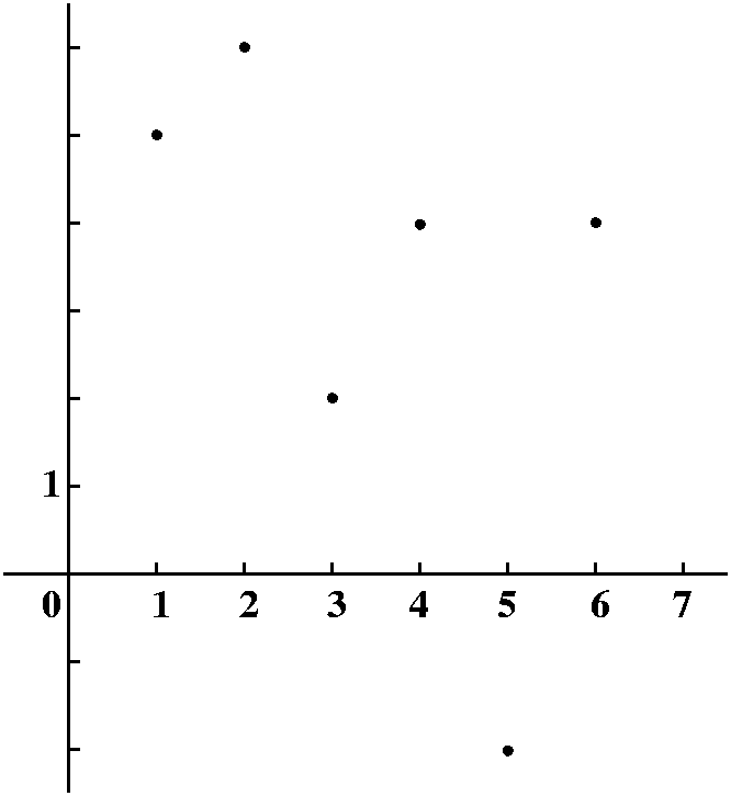
The language and ideas of linear algebra are used everywhere in applied science and engineering. Basic calculus deals fairly nicely with functions defined by formulas involving standard functions. I asked how we could understand more realistic data points. I will simplify, because I am lazy. I will assume that we measure some quantity at one unit intervals. Maybe we get the following:
| Tabular presentation of the data | Graphical
presentation of the data | ||||||||||||||
|---|---|---|---|---|---|---|---|---|---|---|---|---|---|---|---|
|
|
|
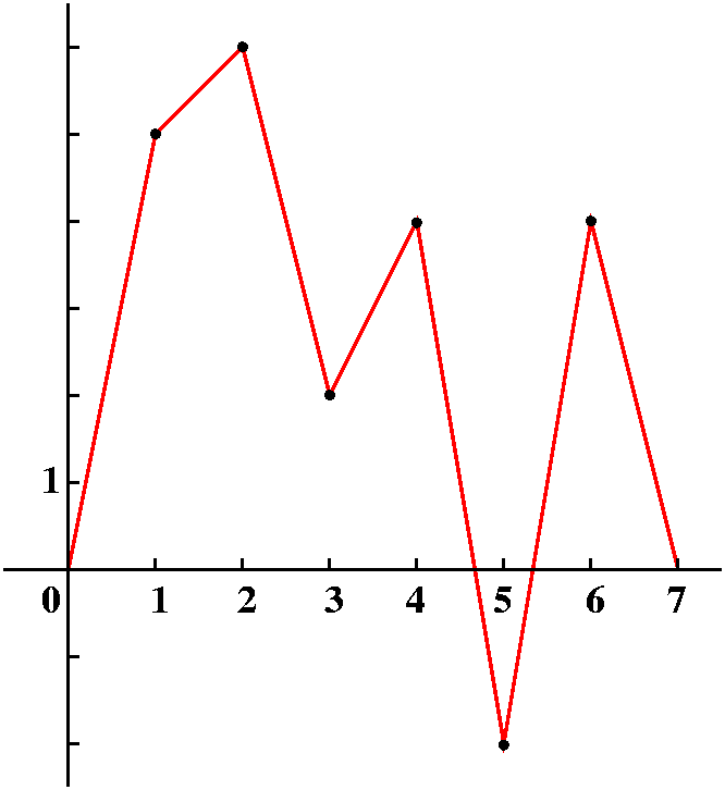
We could look at the tabular data and try to understand it, or we could plot the data because the human brain has lots of processing ability for visual information. But a bunch of dots is not good enough -- we want to connect the dots. O.k., in practice this means that we would like to fit our data to some mathematical model. For example, we could try (not here!) the best fitting straight line or exponential or ... lots of things. But we could try to do something simpler. We could try to understand this data as just points on a piecewise linear graph. So I will interpolate the data with line segments, and even "complete" the graph by pushing down the ends to 0. The result is something like what's drawn to the right. I will call the function whose graph is drawn F(x). |
|
Meet the tent centered at the integer j
First,
here is complete information about the function Tj(x) which
you are supposed to get from the graph of Tj(x): (j
should be an integer)
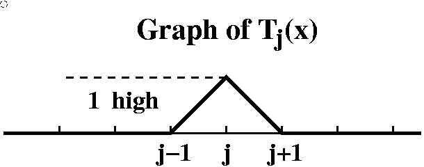
This is a peculiar function. It is 0 for x<j-1 and for x>j+1. It has height 1 at j, and interpolates linearly through the points (j-1,0), (j,1), and (j+1,0). I don't much want an explicit formula for Tj(x): we could clearly get one, although it would be a piecewise thing. Actually, Tj(x) could be written nicely in Laplace transform language!
We can write F(x) in terms of these Tj(x)'s. Moving (as we
were accustomed in Laplace transforms!) from left to right, we first
"need" T1(x). In fact, consider 5T1(x) and
compare it to F(x). I claim that these functions are exactly
the same for x<=1. Well, they are both 0 for x<=0. Both of these
functions linearly interpolate between the points (0,0) and (1,5), so
in the interval from 0 to 1 the graphs must be the same (two points
still do determine a unique line!). Now consider
5T1(x)+6T1(x) and F(x) compared for x's less
than 2. Since T2(x) is 0 for x<1, there is no interference in
the interval (-infinity,1]. But between 1 and 2, both of the "pieces"
T1(x) and T2(x) are non-zero. But the sum of
5T1(x)+6T1(x) and F(x) match up at (1,5) and
(2,6) because we chose the coefficients so that they would. And both
of the "tents" are degree 1 polynomials so that their sum is also, and
certainly the graph of a degree 1 polynomial is a straight line, so
(again: lines determined by two points!) the sum
5T1(x)+6T1(x) and F(x) totally agree in the
interval from 1 to 2. Etc. What do I mean? Well, I mean that
F(x)= 5T1(x)+6T1(x)+2T1(x)+4T1(x)+
-2T1(x)+4T1(x).
These functions agree for all x.
Linear combinations of the tents span these piecewise linear
functions
If we piecewise linearly interpolate data given at
the integers, then the resulting function can be written as a linear
combination of the Tj's. Such linear combinations can be
useful in many ways (for example, the definite integral of F(x) is the
sum of constants multiplied by the integrals of the Tj(x),
each of which has total area equal to 1!). The Tj(x)'s are
enough to span all of these piecewise linear functions.
But maybe we don't need all of the Tj's. What if someone
came up to you and said, "Hey, you don't need T33(x) because:"
T33(x)=53T12(x)-4T5(x)+9T14(x)
Is this possibly correct? If it were correct, then the function
T33(x) would be redundant (extra, superfluous) in our
descriptions of the piecewise linear interpolations, and we wouldn't
need it in our linear combinations. But if
T33(x)=53T12(x)-4T5(x)+9T14(x)
were correct, it should be true for all x's. This means we can
pick any x we like to evaluate the functions, and the resulting
equation of numbers should be true. Hey: let's try x=33. This is not
an especially inspired choice, but it does make T33's value
equal to 1, and the value of the other "tents" in the equation equal
to 0. The equation then becomes 1=0 which is currently
false.
Therefore we can't throw out
T33(x). In fact, we need every Tj(x) (for each
integer j) to be able to write piecewise linear interpolations.
We have no extra Tj(x)'s: they are all
needed.
Let me rephrase stuff using some linear algebra language. Our "vectors" will be piecewise linear interpolations of data given at integer points, like F(x). If we consider the family of "vectors" given by the Tj(x)'s, for each integer j, then:
- This family spans every thing. Every piecewise linear function is a sum of scalar multiples of the Tj(x)'s.
- This family is linearly independent. We need each member, each specific Tj(x), in order to be able to write any F(x) as a linear combination of the Tj(x)'s.
I emphasized that one reason I wanted to consider this example first is because we use linear algebra ideas constantly, and presenting them in a more routine setting may discourage noticing this. My second major example does, however, present things in a more routine setting, at least at first.
My "vectors" will be all polynomials of degree less than or equal to 2. So one example is 5x2-6x+(1/2). Another example is -(Pi)xx2+0x+223.67, etc. What can we say about this stuff?
I claim that every polynomial can be written as a sum of 1 and x and
x2 and the Clark polynomial, which was something like
C(x)=3x2-9x+2. It was generous of Mr. Clark to volunteer his polynomial. I
verified that, say, the polynomial 17x2+44x-98 could indeed
be written as a sum of 1 and x and x2 and the (fabulous)
Clark polynomial,
C(x)=3x2-9x+2 (well, it was something like
this!). Thus I need to find numbers filling the empty spaces in the
equation below, and the numbers should make the equation correct.
17x2+44x-98=[ ]1+[ ]x+[ ]x2+[ ]C(x)
Indeed, through great computational difficulties I wrote
2+44x-98=-1021+62x+11x2+2C(x)
(I think this is correct, but again I am relying upon carbon-based
computation, not silicon-based computation!)
We discussed this and concluded that the span of 1 and x and
x2 and C(x) is all the polynomials of degree less
than or equal to 2. But, really, do we need all of these? That is, do
we need the four numbers (count them!) we wrote in the equation above,
or can we have fewer? Well, 1 and x and x2 and C(x)
are not linearly independent. They are, in fact, linearly
dependent. There is a linear combination of these four which is
zero. Look:
1C(x)+(-3)x2+(9)x+(-2)1=0.
so that
C(x)=3x2+-9x+21
and we can "plug" this into the equation
17x2+44x-98=-1021+62x+11x2+2C(x)
to get
17x2+44x-98=-1021+62x+11x2+2(3x2+-9x+21)
But a linear combination of linear combinations is also a linear combination (they concatenate well). So {1,x,x2,C(x)} certainly span the quadratic polynomials, but so does {1,x,x2}. We also notice that {1,x,C(x)} spans everything. But are there any more redundancies? Does {1,C(x)} span all quadratic polynomials? Mr. Mostiero suggested that I try to write 1+x2 as (scalar)1+(another scalar)C(x). In order to get the x2 term, I need "another scalar" to be not zero. But then the sum (scalar)1+(another scalar)C(x) must have a term involving x, and therefore cannot be equal to 1+x2.
We could sort of diagram what's going on. There seem to be various levels. The top level, where the collections of "vectors" are largest, are spanning sets. Certainly any set bigger than a spanning set is also a spanning set! Now shrink the set to try eliminate redundancies, extra "vectors" that you really don't need for descriptions. There may be various ways to do this shrinking. Clearly (?) you can continue shrinking until you eliminate linear dependencies, and the result will be a linearly independent set. Once the set is linearly independent, then even smaller sets will be linearly independent. But if you continue shrinking, you may lose the spanning property. You may not be able to describe everything in terms of linear combinations of the designated "vectors".
Spanning (with redundancy)         {1,x,x2,C(x)}   SPANNING!
                                    /    \         SPANNING!
                                   /      \        SPANNING!
Spanning, no redundancy     {1,x,x2}    {1,x,C(x)} SPANNING! LINEARLY INDEPENDENT!
(linearly independent)                       |               LINEARLY INDEPENDENT!
                                             |               LINEARLY INDEPENDENT!
                                             |               LINEARLY INDEPENDENT!
Not spanning (not big                    {1,C(x)}            LINEARLY INDEPENDENT!
enough)
There's sort of one level where spanning and linearly
independent overlap. That's the collections of "vectors"
where everything can be described by linear combinations and there are
no redundancies.
Some weird polynomials to change our point of view
Look at these polynomials of degree 2:
P(x)=(x-1)(x-2)
Q(x)=(x-1)(x-3)
R(x)=(x-2)(x-3)
Why these polynomials? Who would care
about such silly polynomials?
Are these polynomials linearly independent?
This was the QotD. I remarked that I was asking students to
show that if
A P(x)+B Q(x)+C R(x)=0
for all x, then the students would need to deduce that A=0 and B=0 and
C=0.
- What I expected from students in their answers
Well, take the equation A P(x)+B Q(x)+C R(x)=0 and plug in x=1. Then we get (since P(1)=0 and Q(1)=0 and R(1)=2) that 2C=0 so that C must be 0. Similarly, x=2 gives B=0 and x=3 gives A=0. So the linear combination is the trivial linear combination, and the polynomials are linearly independent. - What I was doing while the students were writing
At the board I computed P(x)=x2-3x+2 and Q(x)=x2-4x+3 and R(x)=x2-5x+6. Then I wrote the equation
A P(x)+B Q(x)+C R(x)=0
as the equation A (x2-3x+2)+B (x2-4x+3)+C (x2-5x+6)=0
and then I further distributed and got:
(A+B+C)x2+(-3A-4B-5C)x+(2A+3B+6C)=0
which results in the linear system1A+1B+1C=0 -3A-4B-5C=0 2A+3B+6C=0
and then I row reduced (by hand!) the coefficient matrix:( 1 1 1 ) ( 1 1 1 ) ( 1 0 1 ) ( 1 0 0 ) (-3 -4 -5 )~( 0 -1 -2 )~( 0 1 2 )~( 0 1 0 ) ( 2 3 6 ) ( 0 1 4 ) ( 0 0 2 ) ( 0 0 1 )
This shows that the original system was row equivalent to the system A=0 and B=0 and C=0 (remember that "row equivalent"<==>"same solution set"), therefore there are no solutions to the equation A P(x)+B Q(x)+C R(x)=0 except the trivial solution. And therefore P(x) and Q(x) and R(x) are linearly independent: none of them are "redundant".
But can I describe all of the deg<=2 polys this way?
I assert that every polynomial of degree less than or equal to
2 can be described as a linear combination of P(x) and Q(x) and
R(x). How would I verify this claim? Please note that
I am more interested in the logic than the computational details
here!
I should be able to write x2 as sum of P(x) and Q(x) and
R(x). This means I should be able to solve the equation
A P(x)+B Q(x)+C R(x)=x2.
Just as above, this leads to an augmented matrix which looks like:
( 1  1  1 | 1 )   ( 1  0  0 | FRED   )
(-3 -4 -5 | 0 )~~~( 0  1  0 | MARISSA)
( 2  3  6 | 0 )   ( 0  0  1 | IRVING )
I know this is true, since I already did the row operations above. Right now I am not totally interested in the values of FRED and MARISSA and IRVING but I know that the row operations just involve adding and multiplying and interchanging, so there must be such numbers. And therefore there are numbers which satisfy the equation:
FRED P(x)+MARISSA Q(x)+IRVING R(x)=x2.
Therefore x2 is in the span of P(x) and Q(x) and R(x). What about x? The system of equations which results has augmented matrix
( 1  1  1 | 0 )
(-3 -4 -5 | 1 )
( 2  3  6 | 0 )
and just as before there will be solutions, and so x is in the span of P(x) and Q(x) and R(x). And so is 1. Since the linear combinations of x2 and x and 1 are all of the polynomials of degree 2 or less, and each of x2 and x and 1 is a linear combination of P(x) and Q(x) and R(x), I know that the span of P(x) and Q(x) and R(x) is all polynomials of degree 2 or less. So each of P(x) and Q(x) and R(x) is needed and there are "enough" of them. Notice that all I needed to do was verify that the RREF of the matrix above was in the 1 0 0 etc. form. Then everything automatically followed!
|
|
So P(x) and Q(x) and R(x) are a basis of the polynomials of degree less than or equal to 2.
Why would we look at P(x) and Q(x) and
R(x)?
Suppose again I have data points, let's say (1,13) and (2,18) and
(3,-9). I could do linear interpolation as we did above. If I want to be
a bit more sophisticated, and get maybe something smoother, I could
try to get a polynomial Ax2+Bx+C which fits these data
points. Here is the polynomial:
[-9/2]P(x)+[18/-2]Q(x)+[13/-2]R(x). How was this remarkable
computation done? Well, I know certain function values
| The function | Its values when x=1 and x=2 and x=3 | ||
|---|---|---|---|
| P(x) | 0 | 0 | 2 |
| Q(x) | 0 | -1 | 0 |
| R(x) | 2 | 0 | 0 |
so when I "plug in" x=1 and x=2 and x=3 in the linear combination A P(x)+B Q(x)+C R(x) and I want to get 13 and 18 and -9, respectively, the structure of the table makes it very easy to find A and B and C. If we want to interpolate quadratically, I would get a function defined by a simple formula using this basis. In fact, these functions are very useful in quadratic interpolation, and in the use of splines, a valuable technique for numerical approximation of solutions of ordinary and partial differential equations.
HOMEWORK
An exam is coming. Please look at the review
material. I will be in Hill 525 at 4 PM on Sunday.
|
Monday, October 3 |
|
3x1+2x2+x3-x4=A
4x1-1x2+5x3+x4=B
2x1+5x2-3x3-3x4=C
These questions will be important:
- For which values of A and B and C does this system have any solutions?
- If A and B and C have values for which there are solutions, describe the solutions in some effective way.
(3  2  1 -1 | A)
(4 -1  5  1 | B)
(2  5 -3 -3 | C)
The vertical bar is used to distinguish between the two sides of the equations. It is useful to change the collection of linear equations so that the system becomes easier to understand. These changes should all be reversible, so that these equivalent systems will have the same set of solutions.
- Any initial non-zero entry in each row is 1.
- The other column entries for an initial non-zero entry of 1 will be 0.
- Initial 1's to the right always occur in lower rows. That is, if aij is an initial 1 and amn is another initial 1, then if i<m, j must be <n.
 3 by 4         2 by 7
(1 0 0 0)   (1 0 0 0 0 4 4)
(0 0 1 5)   (0 0 0 0 1 2 3)
(0 0 0 0)
And here is essentially a complete list of all possible 3 by 3 RREF matrices:
(1 0 0)  (1 0 *)  (1 * *)  (1 * 0)  (0 1 0)  (0 1 *)  (0 0 1)  (0 0 0)
(0 1 0)  (0 1 *)  (0 0 0)  (0 0 1)  (0 0 1)  (0 0 0)  (0 0 0)  (0 0 0)
(0 0 1)  (0 0 0)  (0 0 0)  (0 0 0)  (0 0 0)  (0 0 0)  (0 0 0)  (0 0 0)
The entries * may be any number, 0 or non-zero. There aren't very many and they are easy to understand. Notice that each of these is essentially different from the others: they represent coefficient matrices with very different solution sets.
My example
I then tried to use row operations on the augmented matrix of my
system of linear equations so that the coefficient matrix was in
RREF. I did this by hand. What follows is taken from a Maple
session (I did remove my errors!). Maple does have a
rref command, but it also allows row operations one at a
time. I will comment in this manner
about each command.
>with(linalg):
This loads the linear algebra package.
>M:=matrix(3,5,[3,2,1,-1,A,4,-1,5,1,B,2,5,-3,-3,C]);
                        [3     2     1    -1    A]
                        [                        ]
                   M := [4    -1     5     1    B]
                        [                        ]
                        [2     5    -3    -3    C]
This command just creates a matrix of specified size
with the listed entries.
>mulrow(M,1,1/3);
                   [1    2/3    1/3    -1/3    A/3]
                   [                              ]
                   [4    -1      5      1       B ]
                   [                              ]
                   [2     5     -3      -3      C ]
Multiply row 1 by a third. Creates an initial 1.
>addrow(%,1,2,-4);
              [1     2/3     1/3     -1/3       A/3   ]
              [                                       ]
              [                                4 A    ]
              [0    -11/3    11/3    7/3     - --- + B]
              [                                 3     ]
              [                                       ]
              [2      5       -3      -3         C    ]
Add -4 times row 1 to row 2. This "pivots" and makes the
(2,1) entry of the coefficient matrix 0.
>addrow(%,1,3,-2);
              [1     2/3      1/3     -1/3       A/3   ]
              [                                        ]
              [                                 4 A    ]
              [0    -11/3    11/3     7/3     - --- + B]
              [                                  3     ]
              [                                        ]
              [                                 2 A    ]
              [0    11/3     -11/3    -7/3    - --- + C]
              [                                  3     ]
Add -2 times row 1 to row 3. So the (3,1) entry becomes 0.

>mulrow(%,2,-3/11);
              [1    2/3      1/3     -1/3       A/3   ]
              [                                       ]
              [                       -7     4 A   3 B]
              [0     1       -1       --     --- - ---]
              [                       11     11    11 ]
              [                                       ]
              [                                2 A    ]
              [0    11/3    -11/3    -7/3    - --- + C]
                                                3
Makes another leading 1.
>addrow(%,2,1,-2/3);
              [                               A     2 B]
              [1     0        1      1/11    ---- + ---]
              [                               11    11 ]
              [                                        ]
              [                       -7     4 A   3 B ]
              [0     1       -1       --     --- - --- ]
              [                       11     11    11  ]
              [                                        ]
              [                                2 A     ]
              [0    11/3    -11/3    -7/3    - --- + C ]
              [                                 3      ]
Makes the (1,2) entry equal to 0.
>addrow(%,2,3,-11/3);
                [                          A     2 B ]
                [1    0     1    1/11     ---- + --- ]
                [                          11    11  ]
                [                                    ]
                [                 -7      4 A   3 B  ]
                [0    1    -1     --      --- - ---  ]
                [                 11      11    11   ]
                [                                    ]
                [0    0     0     0      -2 A + B + C]
And now the (3,2) entry is 0. The coefficient matrix
is now in RREF.
Well, this went a heck of a lot better than when I did it in class. I
will try, as I said, to avoid doing very much row reduction in
class. I am totally inept at it.
Now back to the questions:
- For which values of A and B and C does this system have any solutions?
- If A and B and C have values for which there are solutions, describe the solutions in some effective way.
What if I know -2A+B+C=0? It turns out that there are solutions: the system is consistent. Let me check this claim by choosing some values of A and B and C which will make -2A+B+C=0 true. How about A=4 and B=3 and C=5? Then -2A+B+C=-2(4)+3+5=0 (I hope). The RREF system then becomes (inserting these values of A and B and C [I did this in my head so there may be ... errors]):
                [                          10  ]
                [1    0     1    1/11     ---- ]
                [                          11  ]
                [                              ]
                [                 -7        7  ]
                [0    1    -1     --    - ---- ]
                [                 11       11  ]
                [                              ]
                [0    0     0     0         0  ]
Then the first equation (unabbreviated) is
x1+x3+(1/[11])x4=([10]/[11]) so thatx1=-x3-(1/[11])x4+([10]/[11]).
Similarly the second equation becomes
x2=x3+(7/[11])x4-([7]/[11]).
Be sure to look carefully at the signs, to check on what I've written. The equations have been written this way so that you can see that x3 and x4 are free. That is, I can give any values for these variables. Then the other variables (x1 and x2) will have their values specified by what is already given. So: we select A and B and C satisfying the compatibility condition. Then there always will be a two-parameter family of solutions to the original system of linear equations. Notice that we get solutions exactly when the compatibility condition is satisfied: there are solutions if and only if (as math folks might say) the compatibility condition is correct.
The logic here is actually "easy". Since all the computational steps we performed are reversible, I know that the assertions I just made are correct. What is more wonderful is that the general situation will always be much like this.
What RREF does in general
Take your original augmented matrix, and put
the coefficient matrix into RREF. Then you get something like
(BLOCK OF 1's & 0's WITH|  JJJJJJ  UU  UU  NN  N  K K | Linear stuff )
(THE 1's MOVING DOWN AND|    JJ    UU  UU  N N N  KK  | from original)
(TO THE RIGHT.          |  JJJJ    UUUUUU  N  NN  K K |  right sides )
(--------------------------------------------------------------------)
(                    MAYBE HERE SEVERAL               |   More such  )
(                       ROWS OF 0'S                   | linear stuff )
Please observe that the lower right-hand corner now plays the part of the compatibility conditions which must be satisfied. All of those linear "fragments" must be equal to 0 if the original system has solutions. Now if these are 0, we can "read off" solutions in much the same manner as the example. The block labeled JUNK in fact tells us with its width how many free parameters there are in the solutions. Notice that the JUNK block could have size 0 (for example, consider the silly system x1=567,672, already in RREF!) and in that case the system would have only one solution.
I then started to examine other systems of linear equations. I had several purposes, and one was to introduce some additional linear algebra vocabulary.
Linear combination
Is (1,2,3,4) a linear combination of (1,1,-1,0) and (1,0,1,1) and (1,0,0,1)?
Suppose v is a vector and w1,
w2, w3, ..., wk
are other vectors. Then v is a linear combination of
w1, w2, ...,wk if
there are scalars c1, c2, ..., ck so
that v=SUMj=1kcjwj
Here v corresponds to (1,2,3,4), and k=3 (there are three
wl;s). Are there scalars (here, just real numbers) so that
(1,2,3,4)=c1(1,1,-1,0)+c2(1,0,1,1)+c3(1,0,0,1)?
Please recognize that this is the same as asking for solutions of
1c1+1c2+1c3=1
1c1+0c2+0c3=2
-1c+1c2+0c3=3
0c1+1c2+1c3=4
This isn't what I did in class, but then I did something easier in class. I will change the coefficient matrix to RREF form.
                A                 B                 C
( 1  1  1 | 1 )   ( 1  0  0 | 2 )   ( 1  0  0 | 2 )   ( 1  0  0 | 2 )
( 1  0  0 | 2 ) ~ ( 1  1  1 | 1 ) ~ ( 0  1  1 |-1 ) ~ ( 0  1  1 |-1 )
(-1  1  0 | 3 )   (-1  1  0 | 3 )   ( 0  1  0 | 5 )   ( 0  0 -1 | 6 )
( 0  1  1 | 4 )   ( 0  1  1 | 4 )   ( 0  1  1 | 4 )   ( 0  0  0 | 5 )
The tilde, ~, is frequently used to indicate that
systems of equations are equivalent.
A The first row operation I used switched the first and second rows.
B I used the first row to zero out (?) the other entries in the first column. Then
C I used multiples of the second row to zero out the other entries
in the second column.
I decided to stop here even though I didn't complete the row
reduction. Look at the last "equation", or rather, let's look at the
equation represented by the last row. It is
0c1+0c2+0c3=5
This system of linear equations has no solution. The system is
inconsistent. The compatibility condition is not satisfied.
Therefore the answer to the original question:
Is (1,2,3,4) a linear combination of (1,1,-1,0) and (1,0,1,1) and (1,0,0,1)?
is No.
Another linear combination
Can t2 be written as a linear combination of t(t+1) and
t(t-1) and (t-1)(t+1)?
Here there are again three "vectors", w1 and
w2 and w3, but the vectors are
polynomials. Are there numbers c1 and c2 and
c3 so that
t2=c1t(t+1)+c2t(t-1)+c3(t-1)(t+1)?
I can tranlate this into a system of linear of equations:
The t2 coefficients: 1 = 1c1+1c2+1c3
The t1 coefficients: 0 = 1c1-1c2+0c3
The t0 coefficients: 0 = 0c1+0c2-1c3
I could do row reduction, but the last equation tells me that c3=0, and then the second equation tells me that c1=c2 and the first equation says their sum is 1, so that c1=1/2 and c2=1/2 finish a solution to this system of equations.
Therefore the answer to the original question:
Can t2 be written as a linear combination of t(t+1) and
t(t-1) and (t-1)(t+1)?
is Yes.
Linear independence
Are t(t+1) and t(t-1) and (t-1)(t+1) linearly independent?
Suppose w1, w2,
w3, ..., wk are vectors. Then
w1, w2, ...,wk
are linearly independent if whenever
the linear combination v=SUMj=1kcjwj=0,
then all of the scalars cj MUST
be 0. In other words, the vector equation v=SUMj=1kcjwj=0
only has the trivial solution.
This may be the most important definition in linear algebra. It contains an "If ... then ..." statement which should be understood. In geometric terms, you could think that linearly independent vectors point off into different directions. Maybe this makes you happy, but my basic "geometric" intution has definitely deserted me above 47 dimensions!
So I need to consider the equation
c1t(t+1)+c2t(t-1)+c3(t-1)(t+1)+0
and then try to see what this tells me about the cj's. The most
important ingredient here is LOGIC. First let me convert this
polynomial equation into a system of linear equations.
The t2 coefficients: 1 = 1c1+1c2+1c3
The t1 coefficients: 0 = 1c1-1c2+0c3
The t0 coefficients: 0 = 0c1+0c2-1c3
The third equation tells me that c3 must be 0. The second equation tells me that c2=c1, and then the first equation says that 2c1=0 so c1 must be 0 also. And so c2 must be 0. Wow.
Or we could go to the RREF. Here is what Maple says (this is a homogeneous system so I only need the coefficient matrix):
>with(linalg):
> A:=matrix(3,3,[1,1,1,1,-1,0,0,0,-1]);
                                                            [1     1     1]
                                                            [             ]
                                                       A := [1    -1     0]
                                                            [             ]
                                                            [0     0    -1]

> rref(A);
                                                          [1    0    0]
                                                          [           ]
                                                          [0    1    0]
                                                          [           ]
                                                          [0    0    1]
Therefore all of the cj's must be zero.
Therefore the answer to the original question:
Are t(t+1) and t(t-1) and (t-1)(t+1) linearly independent?
is Yes.
Just one more ...
Are the functions cos(t), sin(t), and cos(t-78) linearly independent?
So I'm asking if there are scalars so that
c1cos(t)+c2sin(t)+c3cos(t-78)=0, and the
implication of the question is that this should be true for all t.
There were many complaints. Engineering
students were complaining about the absurdity of 78. There are
many sillier numbers. Also there was little understanding of the
question. Huh ... well, an inspiration arose ... cos(t-78): we can
regress to a more primitive form of life, and recall a trig formula
(which is on the formula sheet
for the first exam!):
cos(A+B)=cos(A)cos(B)-sin(A)sin(B)
If A=t and B=-78, then cos(t-78)=cos(t)cos(-78)-sin(t)sin(-78). So
look at
c1cos(t)+c2sin(t)+c3cos(t-78)=0
and realize (with cos(-78)=cos(78) and sin(-78)=-sin(78)) that
-cos(78)cos(t)-sin(78)sin(t)+cos(t-78)=0
Therefore the answer to the original question:
Are the functions
cos(t), sin(t), and cos(t-78) linearly independent?
is
NO. You could take c1=-cos(78) and
c2=-sin(78) and c3=1. I hope I got the signs right.
Word of the day regress
1. To go back; move backward.
2. To return to a previous, usually worse or less developed state.
QotD
The QotD represents an opportunity for people to earn 5 points on next
week's exam. Also, it allows students to convince me that they can
convert a matrix to RREF. I gave everyone a randomly chosen 3 by 5
matrix, with entries integers between -3 and 3. I asked people to tell
me the RREF of the matrix. Any one who has not earned 5 points for the
exam can try again out of class (in my office, Hill 542, for example).
Here, for the curious, is the Maple code which created these problems:
>with(linalg):
> z:=rand(-3..3);
    z := proc() (proc() option builtin; 391 end proc)(6, 7, 3) - 3 end proc
Creates a "random number" procedure, with output -3,-2,-1,0,1,2,3.
> ww:=(p, q) -> matrix(p, q, [seq(z(), j = 1 .. p*q)]);
            ww := (p, q) -> matrix(p, q, [seq(z(), j = 1 .. p q)])
Creates a p by q matrix with entries random outputs of the procedure z
previously defined.
> zz:=proc(p, q, A, B) C := ww(p, q); B := rref(C); A:=C; return end;
Warning, `C` is implicitly declared local to procedure `zz`
zz := proc(p, q, A, B)
local C;
    C := ww(p, q); B := linalg:-rref(C); A := C; return
end proc
Creates a matrix and gets its RREF.
> zz(3,5,frog,toad);eval(frog);eval(toad);
                          [1    -2    -1    -1     2]
                          [                         ]
                          [2     0    -1     3    -3]
                          [                         ]
                          [0    -2    -1    -2    -3]

                          [1    0    0     1      5]
                          [                        ]
                          [0    1    0    3/2    -5]
                          [                        ]
                          [0    0    1    -1     13]
One example of the final procedure.
HOMEWORK
Prepare for the exam. Review suggestions are
available.
|
Thursday, September 29 |
|
A linear equation is a sum of scalar multiples of unknown quantities
equal to a scalar. So
A system of linear equations is a collection of linear equations. So
Frequently we will abbreviate a system of linear equations. The actual
variable names (x3 and x44, etc.) may not be
important. The coeffients of the variables (as an ordered set!) and
the constants are important. The system
Matrix algebra
Matrices of the same size can be added.
Matrices can be multiplied by scalars, so that
Matrix multiplication is more mysterious, and why it occurs the way it
does may not be completely obvious. Suppose somehow that quantities
x1 and x2 are controlled by y1
and y2 by the equations
Matrix multiplication is defined only when the "inner dimensions"
coincide. So A·B is defined when A is an n-by-m matrix and B is
an m-by-p matrix. The result, C, is an n-by-p matrix, and
cik=SUMt=1maitbtk:
it is the dot product of the ith row of A by the
jth column of B. This "operation" is important and occurs frequently
enough so that many chip designers have it "hard-wired".
Matrix multiplication is associative but it is not necessarily
commutative. The QotD was to give an example of two 2-by-2
matrices A and B so that AB and BA are not equal.
A solution to a system of linear equations is a n-tuple of scalars
which when substituted into each equation of the system makes the
equation true. The phrase n-tuple is used since I want to have
the scalars ordered as they are substituted> So consider the
system
Here are some linear algebra questions:
Systems of linear equations are frequently analyzed by changing them
to equivalent systems. Two systems are equivalent if they have
the same set of solutions. So, for example, the systems
I want to describe an algorithm which allows us to "read off" whether
solutions of systems exist, and, when they exist, to describe them
efficiently. The algorithm uses
I will show how to use these operations to change a matrix to reduced
row echelon form (RREF). The algorithm is called Gaussian elimination
or row reduction or ...
HOMEWORK
Maintained by
greenfie@math.rutgers.edu and last modified 9/2/2005.
3x1-77x2=408sqrt(17)
is a linear equation.
I will frequently call the unknown
quantities x1, x2, ... etc. So a linear equation
is
41x1-.003x2+Pi x3=98
-x1+0x2-441,332x3=0
is a system of linear equations.
41x1-.003x2+Pi x3=98
-x1+0x2-441,332x3=0
has coefficient matrix equal to
( 41 -.003    Pi    )
( -1    0  -441,332 )
and its augmented matrix
is
( 41 -.003    Pi    | 98 )
( -1    0  -441,332 |  0 )
The use of the vertical bars (|) to separate the coefficients and the constants
is conventional in your textbook and many other places, but not everywhere.
A matrix is a rectangular array. If the number of rows is n and the number of columns is m,
the matrix is said to be nxm (read as "n by m"). If A=(aij) is a matrix with
entries aij, then i refers to the row number and j refers to the cokumn number.
( 2  3 9 1 )   ( 0 9 -4 Pi )   ( 2 12 5 Pi+1 )
( 3 -4 0 7 ) + (10 1 -7 0  ) = (13 -3 -7 7 )
( 5  0 4 12)   ( 3 3  3 3  )   ( 8 3 7 15 )
so if A and B are both n-by-m matrices, the ijth entry of
A+B is aij+bij.
 ( 9 4)   ( 63 28 )
7( Q P) = ( 7Q 7P )
 ( 3 1)   ( 21  7 )
The ijth entry in cA is caij.
3x1-2x2=y1
5x1+7x2=y2
Maybe this is some kind of reaction or linkage or something. Also now
suppose that y1 and y2 are in turn ?controlled
by quantities z1 and z2, and this control is
also expressed by a system of equations:
4y1+15y2=z1
8y1-7y2=z2
How can we expressed the relationship between the pair z1 and z2
and the pair x1 and x2 more directly? Well, we can plug in
the equations for the x's into the equations for the y's:
4(3x1-2x2)+15(5x1+7x2)=z1
8(3x1-2x2)-7(5x1+7x2)=z2
This sort of concatentation of control does occur quite often in many mathematical models. If we multiply through, we see that the equations have become:
(4·3+15·5)x1+(4·-2+15·7)x2=z1
(8·3+-7·5)x1+(8·-2+-7·7)x2=z1
The coefficients combine in sort of a strange way.
    A     ·     B    =      this which is equal to      this
( 4  15 )  ( 3  -2 )      ( 4·3+15·5   4·-2+15·7 )    ( 87  97 )
( 8  -7 )  ( 5   7 )      ( 8·3+-7·5   8·-2+-7·7 )    (-11 -65 )
5x1-x2+2x3=23
7x1+3x2-x1=10
The 3-tuple (triple) of numbers (2,1,7) is a solution to this system. The triple
(0,0,2) is not a solution, and neither is the triple (1,7,2).
Answer It turns out that the answer is "Yes, there are always
other solutions." This does not depend on the number of equations.
Answer In fact, this situation could not possibly be
correct! We will discover why.
Suppose we have a linear system with 235 equations and 517
unknowns. Does this linear system have a non-trivial solution?
Answer In fact, there is actually, always (!) a solution
to this homogeneous system which is not all 0's. I don't think this is
obvious.
5x1-x2+9x3=-17
2x1+33x2-x3=3
10x1-2x2+18x3=-34
6x1+99x2-3x3=9
are equivalent.
Elementary row operations
These are all reversible. About the only subtle observation to make is
about the adjective "non-zero": if we allowed multiplication by 0 we
couldn't reverse the operation.
Please hand in these problems on Monday. I hope they will be graded
and returned to you on Thursday. Maybe this will help with your exam
preparation. So: 4.5: 11, 4.6: 11, 8.1: 37, and 8.2: 6. I strongly
suggest that you don't look in the back of the book for the
answers. Do the problems first!
Further information about the exam will be available soon. There will
be a review session on Sunday, October 9. Further information on that
will also be available soon.