|
Monday, September 26 |
|
It may be useful to understand what this algebraic mess means.
And even more resonance
What if the driving force hits every 2Pi after t=Pi? The mathematical
model is
y´´+Ky´+y=SUMj=0infinitydelta(t-(2j+1))
with,
again, y(0)=0 and y´(0)=0. Let us analyze this as we've already
done. Of course, we could worry about the infinite sum, which
is sort of a limit, but "Almost every reasonable limit should exist."
I won't worry.
Exactly as before, the Laplace transform is
Y(s)=SUMj=0infinity[e-(2j+1)Pi·s]/[s2+1].
This Laplace transform already has built into it the initial
conditions and the "rough" inhomogeneity of the forcing term.
The inverse Laplace transform is
y(t)=SUMj=0infinitysin(t-(2j+1)Pi)U(t-(2j+1)Pi).
Again please remember that sine is periodic with period 2Pi. Therefore
sin(t-(2j+1)Pi)=sin(t-Pi), and
y(t)=SUMj=0infinitysin(t-Pi)U(t-(2j+1)Pi)=sin(t-Pi)SUMj=0infinityU(t-(2j+1)Pi).
What's left in the sum is not a constant function, but it is a
staircase function (the graph looks more or less like 4.3, #62.
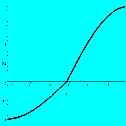
What about the motion? Is it smooth? Where is it smooth? The
graph is a bit difficult to consider for t large, but if we ask
Maple to "zoom in" near a specific t (I think this is t=3Pi)
you can see a kink in the graph. At 3Pi, the slope changes from 1 to
2. And (3+2j)Pi, motion will be continuous (this spring doesn't fly
apart!) but the graph will not be differentiable: slope changes from j
to j+1.
This is a great vocabulary day:
kink
a. a short backward twist in wire or tubing etc. such as may cause
an obstruction.
b. a tight wave in human or animal hair.
jerk
a. a sharp sudden pull, twist, twitch, start, etc.
b. a spasmodic muscular twitch.
c. (in "pl.") [Brit.] [colloq.] exercises ("physical jerks").
d. [sl.] a fool; a stupid person.
And how about limiting the amplitude
Here is a special bonus problem for mechanical
engineering students, and any others who can grasp these concepts. Our
ideal spring y´´+y can have a damping term: y´´+Ky´+y for some real
constant K. This might correspond to the spring vibrating in honey or
10W30 motor oil or ... whatever. Suppose we hit the spring again every
2Pi. I know that the model described above is, indeed, just a
classroom model. It is hard to conceive of Hooke's law applying at the
spring stretches more and more and more (4 light years?). So the
design question: find a value of K so that the spring is limited in
motion (with, say, |y(t)|<10) for a limited time, say
0<t<200. You must give some supporting evidence that your
candidate for K actually restricts the motion in the required
fashion.
Please note that a math person might actually try to compute the exact
solution, and might then investigate the highest value of y(t),
etc. What could an engineer do? Well, maybe build a spring system
(difficult and perhaps expensive). Or find some other nearly
experimental way to verify that a conjectured value of K works.
Hint After class, I returned to my office, and guessed a value
of K, and got good enough verification within 45 seconds, with some help from ...
QotD
I asked people to find a formula for the Laplace transform, Y(s), of
the solution to the Initial Value Problem:
y´´(t)+3y´(t)+y(t)=t+delta(t)
y(0)=1 and y´(0)=-2.
How to do this: I would try to use effectively the dictionary of Laplace transforms displayed on the board. So the equation
y´´(t)+3y´(t)+y(t)=t+delta(t)
becomes:
s22Y(s)-sy(0)-y´(0)+3(sY(s)-y(0))+Y(s)=1/s+e-2s
and, inserting the initial conditions, we get:
s22Y(s)-s+2+3(sY(s)-1)+Y(s)=1/s2+e-2s
and collecting Y(s) terms:
(s2+3s+1)Y(s)-s+2-3=(1/s2)+e-2s
so that
Y(s)=[(1/s2)+e-2s+s+1]/(s2+3s+1).
By the way, amid the general hilarity, I neglected to inform you that my solution which I did half an hour before class, also had an error. Sigh. I then asked the following question, which I believe is useful to think about. Suppose we have this Laplace transform. What sorts of functions should we expect in the inverse transform? It's my hope that you would have a computer algebra system to solve the equation but you should be able to make some rough checks on the answers.
I notice that s2+3s+1 has real roots (the discriminant, 32-4·1·1=5 is positive). Therefore I would not expect sine or cosine. I would expect some sums of exponentials. I would also expect some Heaviside function entry for two reasons: there is a delta in the right-hand side, and we can only get that as a derivative of U, and, second, the e-2s in the transform, which the second translation theorem will turn into a U. Now let's see what Maple answers, assuming I can type correctly.
> with(inttrans): > invlaplace(((1/s^2)+exp(-2*s)+s+1)/(s^2+3*s+1),s,t); / 1/2 1/2 1/2 \ |(-5 + 3) t 5 3 (-5 + 3) t| 1/2 |------------------ - ---------------| (5 - 3) | / 1/2 \ / 1/2 \ | | |5 | |5 | | | 2 |---- - 3/2| 2 |---- - 3/2| | \ \ 2 / \ 2 / / 1/2 -3 + t + 1/5 exp(-------------------------------------------------) (10 + 3 5 ) / 1/2 \ | 5 | 4 |- ---- + 3/2| \ 2 / / 1/2 1/2 \ 1/2 | (5 + 3) (t - 2) (5 - 3) (t - 2) | + 1/5 5 |-exp(- ------------------) + exp(------------------)| Heaviside(t - 2) \ 2 2 / / 1/2 1/2 1/2 \ | (5 + 3) t 5 3 (5 + 3) t | 1/2 |- ----------------- - ----------------| (-5 - 3) | / 1/2 \ / 1/2 \| | | 5 | | 5 || | 2 |- ---- - 3/2| 2 |- ---- - 3/2|| \ \ 2 / \ 2 // 1/2 - 1/5 exp(----------------------------------------------------) (-10 + 3 5 ) / 1/2 \ |5 | 4 |---- + 3/2| \ 2 /What a mess, but, qualitatively, the guesses above are verified. I think. Section 4.6 in 4.6 minutes
dx dy 2-- + -- -2x = 1 dt dt dx dy -- + -- -3x -3y = 2 dt dt x(0)=0 and y(0)=0This is a textbook problem, so it will not be very difficult (maybe). And this one was rehearsed (!). You may be able to see various ways to solve this problem, but let me be obedient to chapter 4, and use Laplace transforms.
Here are the Laplace transforms of the equations, with the rather silly initial conditions used.
2sX(s)+sY(s)-2X(s)=(1/s) sX(s)+sY(s)-3X(s)-3Y(s)=(2/s)Let's collect things:
(2s-2)X(s) + sY(s) = (1/s) (s-3)X(s) + (s-3)Y(s) = (2/s)Now this is a system of two linear equations in two unknowns. I will divide the first equation by (2s-2):
1X(s) + (s/[2s-2])Y(s)=(1/[s[2s-2])and now I will multiply the modified first equation by (s-3) and subtract it from the second equation. This is resulting second equation:
0X(s) + ((s-3)-(s-3)(s/[2s-2]))Y(s)=(2/s)-(s-3)(1/[s[2s-2])Wow! Now I have isolated Y(s) and can divide by its coefficient, so that
(2/s)-(s-3)(1/[s[2s-2]) Y(s) = ------------------------ ((s-3)-(s-3)(s/[2s-2]))
Maple tells me this:
> invlaplace(((2/s)-(s-3)*(1/(s*(2*s-2))))/((s-3)-(s-3)*(s/(2*s-2))),s,t); - 1/6 + 8/3 exp(3 t) - 5/2 exp(2 t)which is actually the answer in the back of the book. As I mentioned in class, I had to try four times to type the input correctly, matching the parentheses. But let me show you how to find the inverse Laplace transform "by hand".
I will multiply top and bottom by s(2s-2). I will also "factor out" the s-3 in the bottom.
(2/s)-(s-3)(1/[s[2s-2]) 2(2s-2)-(s-3) Y(s) = ----------------------- = ------------------ ((s-3)-(s-3)(s/[2s-2])) (s-3)(s(2s-2)-s2)The top: 2(2s-2)-(s-3)=4s-4-s+3=3s-1.
3s-1 A B C A(s-2)s+B(s-3)s+C(s-3)(s-2) Y(s) = ----------- = --- + --- + - = --------------------------- (s-3)(s-2)s s-3 s-2 s (s-3)(s-2)sand 3s-1=A(s-2)s+B(s-3)s+C(s-3)(s-2). Plug in s=0 to get C=-1/6, plug in s=2 to get B=-5/2, and plug in s=3 to get A=8/3. The answer will be what the book and Maple predicted.
I could get X(s) by putting the complicated rational function description of Y(s) in the equation 1X(s) + (s/[2s-2])Y(s)=(1/[s[2s-2]) and then solving for X(s). I am lazy and won't do this. Last year I discussed a simpler example.
What's going on?
Those students who have some background in linear algebra might see
some sort of pattern. I was doing row reduction in the system of
linear equations given for X(s) and Y(s). I was thinking of various
functions involving s as the scalars (!). My goal was to get 1
and 0 as scalars.
Linear algebra ...
Linear algebra is a subject which involves both scalars and
vectors. Let me tell you about both of them, from an
"operational" point of view.
Here are some examples of scalars and vectors.
HOMEWORK
I would like to give an exam in two weeks, on Monday, October 10. The exam would cover
our work on Laplace transforms and some basic linear algebra. Please
check
the draft version of a formula sheet for the first exam and
give me comments.
The exam will cover what we've done on Laplace transforms and two
lectures on linear algebra, so you probably should read ahead about
linear algebra (see the syllabus & textbook
problems.
Further information about the exam will be available soon.
|
Thursday, September 22 |
|
A simple mechanics problem
I asked people to consider the frictionless eraser.
I tried to slide an eraser along the narrow shelf at the bottom of the
blackboard, asking people to imagine there was no friction. My
mathematical analysis (!) of this problem used F=ma, a wonderful
equation. So here we go: I use F=ma. I will assume that we are
analyzing the motion of a particle on a line. At time t, the particle
is at x(t). I will also assume (since this is a very simple
model!) that m=1 for all time t. If the particle starts from 0 at time
0 with velocity 0, the initial conditions are x(0)=0 and
x´(0)=0. The force will vary with time. What can one expect of such a
problem?
Then setup
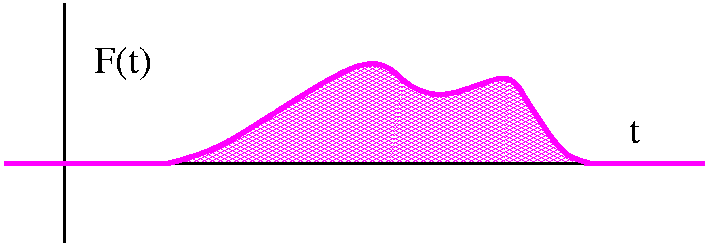
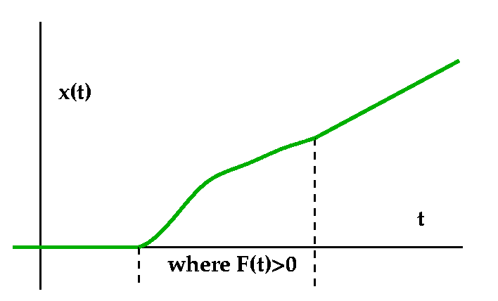
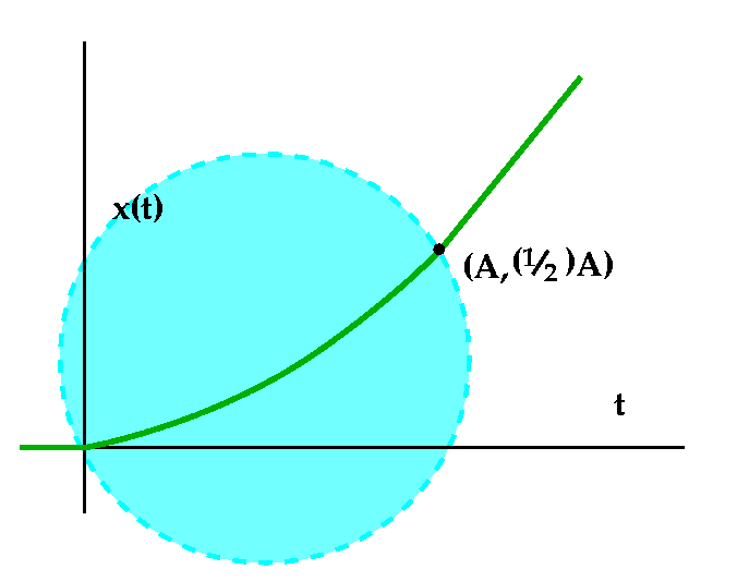
Here's an example of a possible force varying with time, t. Initially, the particle would not move. Then, yes, indeed!, it moves as t increase (once t gets to the region where F(t)>0). Since F(t)>0 there, the particle moves to the right, or (if we consider a graph of t, time, versus, x(t), position) "up". Here is what a graph of x(t) might look like, qualitatively. What is happening? For early time, before the bump in F(t), the particle doesn't move at all. After the bump in F(t), the particle does move, and the amount of movement, it turns out, depends only on the total area under the bump. The total area determines the slope. The particle moves at uniform speed because there is no new force acting on it. What doess the total area represent? Well, work is force·distance, but this is essentially force·time, which in this setup is momentum. (Why? Since x´´(t)=F(t), x´(t)=p(t), the momentum (remember here m=1 always). Thus p´(t)=F(t), and the total area under the F(t) is the change in momentum, as Mr. Wolf suggested. Professor M. Kiessling, a wonderful mathematical physicist, helped (forced?) me to agree to this. In this simple setup, I think that work=energy and momentum gained are proportional. In any case, after the bump, the curve showing positive is linear, with a positive slope. The slope is directly proportional to the total net area. |
|
The example
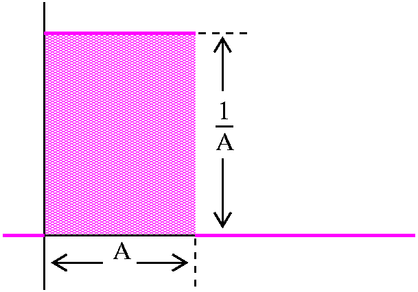
The setup Suppose the graph of F(t) is as shown. Let's find the motion of the point. Since x´´(t)=F(t) with x´(0)=0 and x(0)=0, and this is Math 421, we should use the Laplace transform. Well, we can write F(t) in a suitable form: F(t)=(1/A)U(t)-(1/A)U(t-A). Then take the Laplace transform of x´´(t)=F(t) and get, on the left-hand side (with initial conditions built in), s2X(s)-sx´(0)-x(0). On the right, we will get (1/A)(e-0·s/s)-(1/A)(e-As/s). Therefore we have s2X(s)=(1/A)[1-e-As]/s and X(s)=(1/A)1/s3-(1/A)e-As(1/s3). We now take the inverse Laplace transform. You will need to know the table and the second translation theorem! x(t)=(1/A)(1/2)t2-(1/A)(1/2)(t-A)2U(t-A). For 0<t<A, x(t)=(1/A)(1/2)t2. Since (t-A)2=t2-2At+A2, after some algebra (!!), we see that if t>A, x(t)=(1/A)(1/2)(2At-A2)=(1/2)(2t-A)=t-A/2. It can be checked that x(A)=A/2 for either definition, so the motion is continuous (the eraser didn't suddenly and magically jump!) and actually, the function described is differentiable: the tangent lines agree at the "splices" (t=0 and t=A). A graph of the position is shown. | |
Limits of the motion and what we expect
What happens now as A-->0? |
Dirac delta "function"
Dirac,
a Nobel prize-winning mathematical physicist, worked on quantum
mechanics and relativity. Here is an interesting quote from Dirac: "I
consider that I understand an equation when I can predict the
properties of its solutions, without actually solving it." A contemporary interview with Dirac may
give some idea of his personality.
The Dirac delta function is the limit of these square impulse functions as A-->0+. The Dirac delta function, delta(t), is 0 away from 0. Its total integral is 1. You should think about it as an instantaneous bump, a limit of the boxes above as A-->0. I computed some integrals. They resembled the following:
I computed
the integral -30040delta(t-2) dt: this
was 1.
The integral -300-200delta(t-2) dt was
0. The bump or impulse was centered at 2, and 2 is not in the interval
from -300 to -200.
I tried some further computations. I think one was something like -30040delta(t-2)(t2-5t) dt.
Since the delta function is 0 away from 2, only what multiplies
it at (or close to) 2 matters. But close to 2, the function
t2-5t is close to 4-10=-6. Therefore this integral is just
-6.
The Laplace transform of delta
Another thought about delta
If we multiply fepsilon´(t) by a continuous
function g(t), in the small interval (a really small interval!)
g(t) will hardly vary and will be almost equal to g(0). So the
integral of fepsilon´(t)g(t) will be approximately g(0) multiplied
by the integral of fepsilon, which is 1, so the result is
approximately g(0). Thus fepsilon´(t) is approximately delta(t).
So as epsilon-->0+, fepsilon-->U and
fepsilon´-->delta.
So, "clearly"
U´=delta.
A traditional mixing problem
I wanted to make the Chem E's happy. Here is a two-part problem which
I found last year. It is from an
essay by Kurt Bryan of the Rose-Hulman Institute of Technology:
In fact, the Laplace transform of delta(t-t0) is
easy. We need to compute 0infinitye-stdelta(t-t0) dt. But
the delta only notices the amplitude of the function
multiplying it when delta's argument is 0, so the value of this
integral is e-t0s.
Remember:
Almost every reasonable
function should have a derivative.
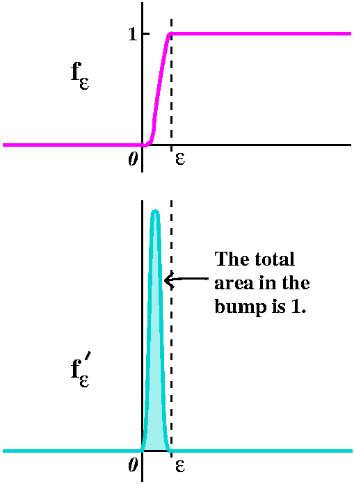
Let's approximate U(t) by
another function, fepsilon(t). Here you should think of epsilon as a very small positive number.
For negative t, fepsilon(t)=0. For positive t>epsilon,
fepsilon(t)=1. In a small interval immediately to the right of 0, fepsilon(t)
increases smoothly from 0 to 1. You are supposed to think that fepsilon(t)
closely approximates U(t). Then fepsilon´(t) is a bump localized (?)
in a small interval to the right of 0. The total integral under the
bump is 1, using the Fundamental Theorem of Calculus since
-1037fepsilon´(t) dt=fepsilon(t)]-1037=fepsilon(37)-fepsilon(-10)=1-0=1.
I sketched these ideas here because many people in the engineering and
applied science communicty (physics, chemistry) find them
useful. Maybe you will, also.
A salt tank contains 100 liters of pure water at time t=0 when water begins flowing into the tank at 2 liters per second. The incoming liquid contains 1/2 kg of salt per liter. The well stirred liquid lows out of the tank at 2 liters per second. Model the situation with a first order ODE and find the amount of the salt in the tank at any time. |
I expect students had modeled and solved such problems a number of times in various courses, and certainly in Math 244.
Let m(t) be the kgs of salt in the tank at time t in seconds. We are
given information about how y is changing. Indeed, m(t) is increasing
by (1/2)2 kg/sec (mixture coming in) and decreasing by (2/100)m(t),
the part of the salt in the tank at time t leaving each second. So we
have:
m´(t)=1-(1/50)m(t) and m(0)=0 since there is initially no salt in the
tank.
Students seemed to realize that the solution curve should look like
this: a curve starting at the origin, concave down, increasing, and
asymptotic to m=50. In the long term, we expect about 50 kgs of salt
in the tank. This is easy to solve by a variety of methods, but in
421 we should use Laplace transforms: so let's look at the Laplace
transform of the equation. We get sM(s)-m(0)=(1/s)-(1/50)M(s). Use
m(0)=0 and solve for M(s). The result is M(s)=1/[s(s+(1/50))]. This
splits by partial fractions with some guesses to
M(s)=50[(1/s)-(1/(s+(1/50)))]. It is easy (it should be easy
for you by now!) to find the inverse Laplace transform and write
m(t)=50(1-e-(1/50)t) which is certainly the expected
solution.
Slightly more interesting ...
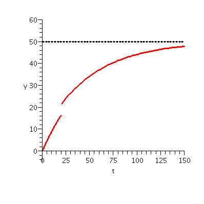
Suppose that at time t=20 seconds 5 kgs of salt is instantaneously dropped into the tank. Modify the ODE from the previous part of the problem and solve it. Plot the solution to make sure it is sensible. |
Students should expect a jump in m(t)
at time 20 of 5, but then the solution should continue to go
asymptotically to 50 when t is large. How should the ODE be modified
to reflect the new chunk of salt? Here is one model:
m´(t)=1-(1/50)m(t)+5delta(t-20) and m(0)=0.
The delta function at t=20 represents the "instantaneous"
change in m(t) at time 20, an immediate impulsive (?) increase in the
amount of salt present.
It is very reasonable to ask if this is a good model. Please keep this is mind!
Back to solving m´(t)=1-(1/50)m(t)+5delta(t-20) and m(0)=0. Take the Laplace transform as before, and use the initial condition as before. The result is now sM(s)-m(0)=(1/s)-(1/50)M(s)+5e-20s from which we get M(s)=50[(1/s)-(1/(s+(1/50)))]+5[e-20s/(s+(1/50))] which has inverse Laplace transform m(t)=50(1-e-(1/50)t)-5U(t-20)e-(1/50)(t-20). Of course I wanted to check my answer, so I used Maple. Here is the command line and here is Maple's response:
> invlaplace(1/(s*(s+(1/50)))+5*exp(-20*s)/(s+(1/50)),s,t); t t -50 exp(- ----) + 50 + 5 Heaviside(t - 20) exp(- ---- + 2/5) 50 50so I am happy. I should remark that last year's version of Maple gave this response:
Some pictures Maple made for me
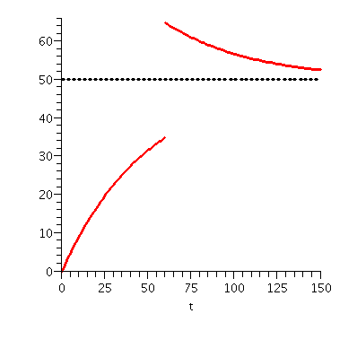
Here's the solution curve for the problem just solved, with an instantaneous increase of 5kg at t=20. The curve jumps up, and then begins to approach 50. | I modified the problem, and dumped in 30 kg of salt at time 60. So you can see the jump above the asymptote, and then the curve trends down towards 50. |
Hitting a spring
Let's look at y´´+y=delta(t-Pi)
with initial conditions y(0)=0
and y´(0)=0. O.k.: to me, what I hope is interesting for the
students in this course is the physical interpretation of
everything. Then we should "solve" it, and then we should consider the
solution from the physical point of view: if it makes sense, this
helps to validate the method we used.
Well: y´´+y models a vibrating spring with no damping, a rather ideal situation. The right-hand side, delta(t-Pi) is a "forcing function". In fact, here it correspods to hitting the spring instantaneously (!) with a "force" of 1 at time Pi. The initial conditions tell us that the spring is originally in equilibrium. At time Pi, the spring is hit but there is no further force (so far). Probably we should expect that the spring will somehow vibrate in an ideal fashion. Let us try our wonderful Laplace routines. The Laplace transform of y´´+y=delta(t-Pi) is s2Y(s)-sy´(0)-y(0)+Y(s)=e-Pi·s which turns out to be (s2+1)Y(s)=e-Pi·s or Y(s)=e-Pi·s/(s2+1). The predicted vibration of the spring is therefore (!) the inverse Laplace transform of e-Pi·s/(s2+1). I can read that off from the (mythical?) table using the second translation theorem and the result is y(t)=sin(t-Pi)U(t-Pi): the spring, responding to an instantaneous load of 1 unit, then vibrates sinusiodally.
Hitting a spring again
Keep the initial conditions the same, but change the forcing function.
So here look at
y´´+y=delta(t-Pi)+delta(t-2Pi). Now go through the
Laplace transform, using the initial conditions:
s2Y(s)-sy´(0)-y(0)+Y(s)=e-Pi·s+e-2Pi·s
becomes
s2Y(s)+Y(s)=e-Pi·s+e-2Pi·s
and then
(s2+1)Y(s)=e-Pi·s+e-2Pi·s
so that
Y(s)=[e-Pi·s+e-2Pi·s]/(s2+1).
The inverse Laplace transform tells me that
y(t)=sin(t-Pi)U(t-Pi)+sin(t-2Pi)U(t-2Pi).
It may be useful to understand what this algebraic mess means.
Confession |
Find the Laplace transform of tU(t-7)
Find the Laplace transform of e-9tt
Mr. Clark intelligently remembered a fact. So he did the following: the Laplace transform of e-9t is
1/(s+9), so the Laplace transform of te-9t is -d/ds[1/(s+9)], and this is 1/(s+9)2.
I needed to be reminded that there are two minus signs in the result and they cancel. Sigh.
Find the Laplace transform of e-5ttU(t-2)
The QotD from last time
Convolution and Laplace transform
Theoretical consequences
What is the convolution of t and t2 and t3 and t4?
What is the convolution of e3t and sin(5t)?
Therefore we will find the convolution of e3t and sin(5t)
by discovering the inverse Laplace transform of
(5/34)/(s-3)-(5/34)s/(s2+25)-(15/34)/(s2+25).
What is the Laplace transform of 0tf(tau)dtau?
$ and *
Textbook problem #43 in section 4.4
We should do this:
Step 1
Back to the problem. We need to find the inverse Laplace transform of
[s3+2s2]/[s4+16].
The poor old prof pooped out (p.o.p.p.o.) here. Well, I can, darn it,
factor s4+16. First, I solve s4=-16. This means
s2=+/-4i, and then another square root gives me
s=sqrt(2)(+/-1+/-i). What the heck is going on? Well, if I want
to do it only with real numbers, I notice that s4+16 is
never 0 (it is always at least 16 for real s's), so it has no real roots.
YUCK!!!
Restated book problem
If any student sees any errors I made, please tell me. Here is a link to a solution of
problem #38 in section 4.4 which I did a year ago. At least I think
it did it correctly! It is similar to the problem I attempted here!
More about the Heaviside function
The Second {Shifting|Translation} Theorem
Since this is a 640 course, I should give some justification of
this result. So I wrote the following:
You don't need to think about this verification again. Just learn how
to use it.
Examples
What about the inverse Laplace transform of, say,
e-3s/s7? This should come from a translated
version of Constant·t6. The -3 part leads to
(t-6)5 but we need to adjust for the proper constant.
So I think this should be
(1/6!)(t-3)6U(t-6).
Another version of the Second {Shifting|Translation}
Theorem
Examples
QotD
Weird formula
Since F(s)=L(f)(s)=0infinitye-stf(t) dt we
could try to differentiate F(s). Thus (d/ds)F(s)=(d/ds)0infinitye-stf(t) dt.
Now push (!) the derivative inside the integral sign:
(d/ds)F(s)=0infinity-te-st\f(t) dt=-0infinitye-stt·f(t) dt
which is minus the Laplace transform of t·f(t).
Therefore the Laplace transform of -t·f(t) is (d/ds)F(s). The
textbook remarks that you can repeat this n times, and the result
is:
I remarked that the interchange of derivative and integral is
not always valid, and manipulations of this sort probably
helped Heaviside get into trouble with the academic
establishment. Look only briefly at the following example which
verifies that the interchange is not always true.
A complicated academic example
What the heck does this function look like? For fixed x it is
continuous in y. For fixed y, it is continuous in x. But it is not continuous in x and y
jointly. Look at the curve y=x^2. So f(t,t^2)=(1/t)e-1, and
that is certainly not continuous at t=0. Slices with y=constant reveal
a bump which gets higher and moves closer to the origin as
y-->0+.
The integral with respect to x can be done easily (the function is
x3e-x2 with various constants thrown
in!). So y=0y=1f(x,y)=xe-x2,
and the derivative of this integral is
e-x2(1-2x2). The value of this at x=0
is 1.
Now the partial derivative of f with respect to x is (for x not equal
to 0) e-x2/y(
3x2/y2-2x4/y3 ). The integral of this mess dy from y=0 to y=1 is
e-x2(1-2x2).
For x=0, the partial derivative is 0 (look at the formula!), and the integral is 0.
Notice now that the integral of the partial derivative with respect to
x at x=0 is 0, but the derivative of the integral of the function with
respect to y at x=0 is 1. These values are not the same!
Convolution
Background
What's the convolution of t2 and t3? This is
0ttau2(t-tau)3dtau.
After a huge amount of debate, we decided (please see here
or here if
this is unfamiliar to you) that (t-tau)3=
1t3-3t2tau1+3t1tau2-1tau3
and therefore
Mr. O'Sullivan suggested the following
web page: http://mathworld.wolfram.com/Convolution.html. It
has a discussion of convolution and an animation picture of several
convolutions.
I need to give more background about this material, and I will.
A textbook problem
Section 4.2, Problem #36 Solve the Initial Value Problem:
As I remarked, this is a very simple ODE: it is second order,
linear, constant coefficient, inhomogeneous. What methods would I
expect/hope that students could use on this problem?
Method #1 First solve the "associated homogeneous equation",
y´´-4y´=0. Plug in ert, get the
characteristic equation,
etc. Attempt to get a particular solution using a variety of methods
(undetermined coefficients or throwing dice or ...).
Method #2 Let y1=y and y2=y´. Build
a column vector
Method #3 Use numerical techniques to approximate a
solution. For many applications, this is just as good. For some
applications such as those requiring long-term asymptotics as a
function of some symbolic initial conditions, for example, numerical
methods aren't too useful. Errors in ODE "stepping" methods (the most
elementary of which is Euler's Method, and one frequently used method
is RKF4, a Runge-Kutta method) tend to accumulta.
Method #4 Use the Laplace transform, which I'll try in a
second. However, there is a natural question: why learn another
method? Well, for this initial value problem almost every method
"works". But each method has its own flavor (?) and gives a different
perspective on the ODE. None of these methods will apply perfectly or
easily or every problem. Having a variety of methods will allow you to
analyze solutions of ODE's better.
So what we do is take the Laplace transform of the entire equation
y´´-4y´=6e3t-3e-t. At this time
please realize that there was a table of Laplace transforms on the
board. So the Laplace transform of the right-hand side is easy, using
linearity and entries in the table. It is [6/(s-3)]+[-3/(s+1)]. What
about the right-hand side? The Laplace transform of the unknown
function, y, is usually written, Y. Then what's the Laplace transform
of y´´?
Laplace transforms of derivatives
This is proved by repeated integration by parts. I verified the n=1
case last time. This result really shows why the Laplace transform is
very well adapted to initial value problems (it was invented
for them, darn it!). Most of the time in this course we will use this
result with n=1 or n=2 but there are certainly lots of cases in
real life with other n's. ME alert n=4: vibrating
beam. Please see example #9 on p.211 of the text.
When n=2, the result states that the Laplace transform of
y´´ is s2Y-sy(0)-y´(0). Here we know that
y(0)=1 and y´(0)=-1 so that the Laplace transform of
y´´ is s2Y-s+1. When n=1, the result states
that the Laplace transform of y´ is sY-y(0). Again using y(0)=1,
we get sY-1 as the Laplace transform of this y´. Therefore (sigh)
the Laplace transform of the left-hand side of the original equation
(y´´-4y´, including the stated initial conditions) is
s2Y-s+1-4(sY-1)=(s2-4s)Y-s+1+4.
So the Laplace transform of
Now what? Now we "solve" for Y, the unknown Laplace transform. And we
attempt to locate pieces of Y on the Laplace transform side of the
table which was on the board. Let's do this.
s2Y-s+1-4(sY-1)=[6/(s-3)]+[-3/(s+1)] becomes
In order to find y(t), we should get the inverse Laplace transform of
Y(s). Using linearity, we "only" need to get the inverse Laplace
transforms of each of the pieces. I think I only analyzed one of the
pieces before I gave up: [6/{(s2-4s)(s-3)}].
So we use partial fractions. The bottom of this fraction is
actually (s-4)s(s-3), so the partial fractions cell in my brain
springs into action: we should be able to write the fraction as the
sum of
I just got Maple 10 at home. This is the same version of
Maple which is in the Rutgers computer labs. Here's a little
bit of the dialogue. # on a line indicates a comment and Maple
ignores it.
Then I gave up, at least computing by hand. But:
I have experience with several different versions of Maple
and they sometimes don't always give the same versions of the
answer. For example, some versions package a linear combination of
e3t and e-3t as an equivalent linear combination
of sinh(3t) and cosh(3t). This can be annoying. I've even found a
version of Maple (not the current one!) which insisted on
using i sinh(i t) instead of sin(t). So using symbolic
manipulation software can have its problems as well as benefits!
What kinds of functions theory interlude #1
As I remarked, polynomials have exponential growth. Maybe that is
"clear" for t2, but not for, say, t216,000. In
fact, I bet that for t large enough positive, |t216,000| is
less than even .003e.000007t. We discussed this, and
decided that this could be verified with L'Hopital's rule. Look at the
quotient
Even something like t216,000e30003t has
exponential growth. It is bounded eventually by some multiple of
e30004t or even just e(30003.001)t.
Here is a candidate suggested by a student (who?) for a function which
does not have exponential growth:
What we're investigating here in Math 421 is the basic, classical
Laplace transform. It has been fiddled with in many ways. So actually
there are ways that functions with faster growth can be used. And
there are ways that, say, difference equations (a discrete analog of
differential equations) can be solved with similar tools. But let's
learn the classical case well enough so that you will be able to use
and understand the variant methods.
Inverse Laplace transforms theory interlude #2
Well, I considered the following example. Certainly our table tells us
that the Laplace transform of t2 is 2/s2. Let's
call t2 by the name, h(t), and let's further define the
function g(t) by the stipulations that g(t) is -1 when t=3 and g(t) is
40 when t=6 and otherwise g(t)=t2. I know the darn picture
is not drawn to scale, but the poetic truth is there. So, anyway,
certainly h and g are distinct functions. But they have the same Laplace transform. Look,
the formula for the Laplace transform of y(t) is 0infinitye-sty(t) dt. And
the integral doesn't even notice if you change the values of
the integrand (the function that's being integrated) at a couple of
points. (Look at the darn definition of the integral, if you don't
believe it, and take a Riemann sum with very, very narrow width around
the jump places.) So there can be two functions whose Laplace
transforms are exactly the same. Well, but for all practical
purposes if you are in a physical situation, you won't notice that
change at a point. And it turns out, more or less, that this is the
only kind of problem you'll face.
Lerch's Theorem (I'm sorry but I like the name.)
Yeah, this can be more precise, but that's all I want to say. But, you
may ask, what if we are supposed to find an inverse Laplace transform?
For example, the inverse Laplace transform of 2/s3? Well,
yeah again, you do have to choose between h(t) and g(t). What everyone
chooses is a function that is as continuous as possible. So if the
left and right-hand limits agree at a point, that's the value the
inverse Laplace transform should have at the point. And the algorithms
in symbolic algebra packages are designed to make such a choice. And
also, there is an inverse Laplace transform with an integral formula,
called Bromwich's integral, which "automatically" gives you the
most continuous (there's a phrase!) inverse Laplace transform. All
these things can be implemented symbolically and numerically.
You can find lots
of references to this stuff on the web.
Our major present goal is to expand our table of Laplace transforms
(and, therefore, inverse Laplace transforms). The two shifting or
translation theorems are very important in accomplishing this.
The first {shifting|translation} theorem
This is correct because the Laplace transform of eatf(t) is
0infinitye-steatf(t) dt
which is the same as
Easy examples
The Heaviside function
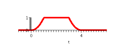
Suppose y(t) is
the function which is 0 for t<0, is t2 for t in the
interval [0,1], is 1 in between 1 and 3, is (t-4)2 in the interval [3,4], and is 0 for "later" t. I hope I've drawn a picture of y(t) to the left.
Here is what Maple does. The first instruction defines the
function, y(t). This uses the builtin function "Heaviside", what we
call U(t). The second instruction plots it. And the plot is shown.
Return of the entrance exam
I hope you will look at this web page. Uhhh ... it is the page you are
looking at now. If you aren't looking at it now, then maybe you could
look at it some time. Or if ... oh well.
I began by reminding people of the definition of Laplace transform.
The Laplace transform of a function y(t) is a function Y(s). Y(s) is
0infinitye-sty(t) dt. This
is also called L(y(t)). Here L means what is usually
written by a calligraphic capital L. It is standard notation
for the Laplace transform.
Laplace transform is linear
Then I copied most of Theorem 4.2 (on p. 193 of the textbook). I
checked that the Laplace transform of eat is 1/(s-a) as the
theorem stated. Here is what we did.
0infinitye-steadt=0infinitye(-s+a)tdt=(Fundamental
Theorem of Calculus, but be careful about what variable you are
"integrating"!)=(1/[-s+a])e(-s+a)t]0infinity.
Now what happens when "t=infinity"? This really means t-->infinity.
So for large enough s (s bigger than a, for example) the exponential
has t multiplied by some constant which is negative. Then the
exponential is decaying so as t-->infinity, the exponential
goes to 0 (more later). When t=0, since we're looking at the bottom
of the ], we have -(1/[-s+a])e0 and e0=1,
so that the answer is-(1/[-s+a]) or 1/s-a, as Theorem 4.1 states.
I wanted to verify the theorem's result for the Laplace
transform of cos(kt). I remarked that the definition tells me that I
need to compute 0inftye-stcos(kt) dt.
Maybe this really isn't too difficult to compute directly.
I would integrate by parts. But
I will need to integrate by parts twice, and the chance for error is
large. Let me show you how to do the computation another way.
Last time I reminded people that cos(theta) is
(1/2)(eitheta+e-itheta). Therefore
the Laplace transform of cos(kt) (so kt will be theta) is
(using linearity of Laplace transform!) is 1/2 multiplied by
the sum of the Laplace transforms of eikt and
e-ikt. The Laplace transform of eikt is 1/[s-ki]
(I'm using the result we just derived, with a changed to ki). The
Laplace transform of e-ikt is 1/[s+ki] (I'm using the
result we just derived, now with a changed to -ki). Therefore the
Laplace transform of cos(kt) is (1/2)({1/[s-ki]}+{1/[s+ki]}). Some
algebra which we did changes this to
(1/2)({[s+ki]+[s-ki]}/{[s-ki][s+ki]}) and this is
(1/2)([2s]/{s2+k2}) which is
s/(s2+k2), the formula I wanted to check.
If you are confused by this, PLEASE try to compute the Laplace
transform of sin(kt) using the same method. PLEASE!!!
A Laplace transform of one little triangle
So Y(s)=01e-sty(t) dt.
Students immediately observed that we don't "need" the integral
where part of the integrand is 0, so we should compute
01e-stt dt. Hey:
this computation demands integration by parts.
Here we can use u=t so dv=e-st dt. Then du=dt and
v=(-1/s)e-st. The integration by parts becomes
One comment to make is that we have replaced the rough function by a
function given by complication combinations of nice smooth
functions. Still, it isn't clear that this is a "win" unless further
good things occur. They will.
Simple Laplace transform asymptotics
Now what about s-->0+? O.k., the exponential
e-st still decreases, but it decreases more slowly. (Uhhhh
... these heurisitics can be made precise -- did you think this was a
math course?). So for more and more t, e-st gets
closer and closer to 1 as s-->0+. When we multiply this by
y(t), the result for lots of t will be close to y(t), and the total
integral will look more and more like the net area (area over
the t-axis counted as positive, under the t-axis as negative) of
y(t). So I think that as s-->0+, Y(s)-->the net area under
all of the y(t) function.
Well let's check both of these asymptotic statements with our little
triangle function. So
Y(s)=(-se-s-e-s+1)/s2. Certainly as
s-->infinity, the e-s terms decay, and the s2 in
the bottom takes care of the 1. So Y(s)-->infinity as s-->infinity.
The Laplace transform of f´(t)
Well, let's start with 0infinitye-stf´(t) dt,
which is the Laplace transform of f´(t). Integration by parts can
be used, with u=e-st and dv=f´(t) dt, so that
du=-s e-stdt and v=f(t). Therefore
L(f´)(s)=-f(0)+sL(f)(s).
Special permissions for math courses can only be gotten by applying on the web.
The standard clerical stuff was done. The information discussed, and
much more, is available here and here.
I began by reviewing very briefly the idea of initial value problems
(IVP's) for ordinary differential equations (ODE's). An ODE is an
equation involving an unknown function of one variable and its
derivatives. For example, y´=2t. A solution to such an equation
is a function which when substituted into the equation makes it
"identically" true. For example, in this simple equation
y=t2+C (any constant C) solves the equation. An initial
condition (IC) is a value, "t0", for which we require the
function to have a certain value, "y0". For example, we
could ask that the solution to this ODE satisfy the IC (3,17). Then we
choose C so that 17=32+C is true: I guess C=8. The
combination of ODE and IC is called an initial value
problem. We expect, due to simple physical examples, that IVP's will
have unique solutions. The independent variable in this course will
frequently be called t for time, so the dependent variable y is a
model of some process which depends on time.
Here is one version of the major theoretical result of the subject, the
This is a wonderful theorem, but its usefulness is definitely
limited. You shouldn't read "into" it any more than is already there.
So let me show this with some examples.
General disclaimer The examples discussed in class will mostly
be very artificial, and chosen so that "hand" computation is
practical.
Example 1 y´=e(t2) and y(0)=0. Then the
solution is y(t)=0te(w2)dw. It turns out
(and it can be proved!) that this integral can't be simplified
or written in terms of any of the standard functions of calculus,
using algebraic means of combination, or even using function
composition.
Generally, it is impossible to write solutions of a
random ODE in terms of familiar functions. Students should know that
this is true, even if we use Maple or Matlab or
Mathematica or ... and it even be very difficult or impractical to
approximate solutions numerically. Sigh. The examples and methods that
are shown here and in Math 244 really are a collection of tricks which
work on many ODE's modeling physical situations. They are not
guaranteed to work on all ODE's, or even all ODE's derived from fairly
simple physical models. But the tricks are very useful in many
examples. Now, back to work.
Example 2 The solutions to y´=ty2 are not
difficult to get (the instructor of course made some errors). This is
a separable ODE. I separated the variables, integrating,
cleared up some algebra, and the solutions seemed to be
y=2/(C-t2).
I verified this in the most direct way possible, by computing y´
and checking that the result was
ty2.
Let's look at some specific solutions. The solution satisfying the IC
(0,100) has C=2/100, so y=2/(.01-t2). The natural domain of
this function is (-1/10,1/10). As t-->1/10-, y-->infinity:
the solution explodes. If the IC is (0,2·104) the solution is
y=2/(.0001-t2) and it has domain (-1/100,1/100). There is
one special case (you need to look critically at the separation of
variables process to spot what goes wrong) but if the initial
condition is (0,0), the solution is y=0 for all t.
The most routine example is y´´+y=0, which is the ODE
modeling an ideal spring using Hooke's law. We can still learn things
from this example! This is a second order ODE (order refers to the
highest number of derivatives needed to write the equation). Here the
trick is to guess a solution: try y=ert. Then
y´´+y=0 becomes magically
ert(r2+1)=0. The exponential function is
never 0. Therefore the guess solves the ODE exactly when
r2+1=0 (I think this is called the characteristic
equation). The roots of this characteristic equation are +/-i.
This is a linear ODE. The particular very very important
qualitative consequence is that sums of solutions of solutions of the
homogeneous equation are solutions, and so are constant multiples of
solutions. Why is this true? Look:
Let's use linearity. y´´+y=0 has solutions eit and
e-it, so if C1 and C2 are any
constants, then
C1eix+C2e-ix must be a
solution. Let me search for a solution satisfying certain initial
conditions. Since y´´+y=0 is a second order equation, the IC's will
generally have two parameters. I want a solution satisfying y(0)=1 and
y´(0)=0. I will call this an initial position solution,
yP. What is it?
If
yP(t)=C1eit+C2e-it
then
yP(t)=iC1eit-iC2e-it.
We can get yP(0)=1 by having C1+C2=1.
We can get yP(0)=0 by having
iC1-iC2=0 which is the same as
C1-C2=0. After
some massive amount of thought, we managed to solve this system of linear equations:
C1=1/2 and C2=1/2.
Therefore yP(t)=[eit+e-it]/2.
Similarly, we can solve the initial value problem y´´+y=0 with y(0)=0
and y´(0)=1, which I'll call the initial velocity solution,
yV(t). It turns out to be
yV(t)=[eit-e-it]/(2i). You should
check this!
Why would one want to know the yP and yV
solutions? Well, they are really neat if you want to "solve" lots of
initial value problems for y´´+y=0. The pattern of initial conditions
(1 and 0, and 0 and 1) allows us to write a solution for the IVP
y(0)=7 and y´(0)=-13. Here it is:
7yP(t)-13yV(t). This is so easy.
Everything I've written is correct, but of course some important
things have not been written! First, writing the solutions as
complex exponentials conceals important features of the solutions. For
example, since y´´+y=0 models simple harmonic motion, the solutions
had better be bounded (they shouldn't grow to infinity in any
fashion). I think springs don't do that. And maybe my formulation of
yP and yV doesn't entirely display this. But we
could compare power series or do other stuff and, in some fashion,
remember Euler's formula and its consequences. So here read this,
please:
What happens if we just change a sign in the ODE? If y´´-y=0,
the characteristic equation becomes r2-1=0 with roots
r=+/-1. Solutions are then
C1et+C2e-t. The solutions
corresponding to the Position and Velocity initial conditions (which I
hope I have convinced you are useful, when combined with linearity, in
solving IVP's are as follows:
If we now consider a "general" second order, linear, constant
coefficient, homogeneous ODE (by the way, each phrase or word I've
just written should make some sense to you and if any do not, you
must review material from 244 -- see the syllabus for suggested reading in our
text), Ay´´+By´+Cy=0 then I can tell you what to expect about the
solutions. If B2-4AC<0, probably sines and cosines will
appear. If B2-4AC>0, the solutions can be written with
coshes and sinhes. There will also be some exponential factors
(damping or otherwise). What happens if B2-4AC=0? It's a
mystery, and you should figure it out.
No, no, no!
This is a complicated definition.
If n is a nonnegative integer, the Laplace transform of tn
is n!/sn+1.
I observed that the Laplace transform is linear: the sum of Laplace
transforms of functions is the Laplace transform of the sum of the
functions, and scalar multiplication also works nicely.
The QotD was: if f(t)=5-3t2+9t7?
HOMEWORK
Maintained by
greenfie@math.rutgers.edu and last modified 9/2/2005.
Use a version of the second translation theorem: the Laplace transform
of g(t)U(t-a) is e-as multiplied by the Laplace transform
of g(t+a). So a=7, and g(t)=t, and g(t+a)=t+7 which has Laplace
transform 1/s2+7/s. The answer is e-7s( 1/s2+7/s).
We need the first translation theorem: the Laplace transform of
eatf(t) is F(s-a). Here a=-9 and f(t)=t. So
F(s)=1/s2, and the desired Laplace transform is
1/(s+9)2. The + occurs because s-a=s-(-9)=s+9.
This problem is vicious (viscous?). It involves a concatenation of
both translation results.
Today's word concatenation
To connect or link in a series or chain.
Let's do this two ways.
So e-5ttU(t-2) becomes e-5t(tU(t-2)).
Now the Laplace transform of tU(t-2) is e-2s(1/s2+2/s). We need to "plug in" s+5 for each s in this answer. The result is
e-2(s+5)( 1/(s+5)2+2/(s+5))
So e-5ttU(t-2) becomes (e-5tt)U(t-2). Now
g(t)=e-5tt and, since a=2 here,
g(t+a)=g(t+2)=e-5(t+2)(t+2)=e-10e-5t(t+2). This
has Laplace transform e-10(1/(s+5)2+2/(s+5)). Finally, to finish the use of the second translation
theorem, we need to multiply by e-2s, so the whole answer
is e-2se-10(1/(s+5)2+2/(s+5)).
Thank goodness the answers agree. I think I would use the first
method, but this is solely a psychological (psychotic?) choice. I wanted to see what a silicon friend would do, so I asked:
> with(inttrans);
[addtable, fourier, fouriercos, fouriersin, hankel, hilbert, invfourier, invhilbert, invlaplace,
invmellin, laplace, mellin, savetable]
> laplace(exp(-5*t)*t*Heaviside(t-2),t,s);
exp(-2 s - 10) (2 s + 11)
-------------------------
2
(s + 5)
The answer has been made "pretty", and I can't tell how it was computed.
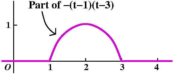
Ms. Jones kindly put her solution on
the board. The given information was a mixture of geometric and
algebraic. The graph of a function was drawn. It was 0 for t<1 and
t>3, and was -(t-1)(t-3) for t between 1 and 3. I asked for the
Laplace transform of this function. I emphasized that it would
probably be easier to begin by describing the function using the
Heaviside function.
We "turn on" -(t-1)(t-3) at 1, and then must remember to turn it off
at 3. So write -(t-1)(t-3)U(t-1)-[-(t-1)(t-3)]U(t-3). This is
-(t-1)(t-3)U(t-1)+[(t-1)(t-3)]U(t-3)
Since Laplace transform is linear, we will work separately with each
piece. And, on each piece, we'll use the second translation theorem:
the Laplace transform of g(t)U(t-a) is e-as multiplied by
the Laplace transform of g(t+a).
For -(t-1)(t-3)U(t-1), we see that a=1, and g(t)=-(t-1)(t-3). So g(t+a)=g(t+1)=-(t+1-1)(t+1-3)=-t(t-2)=-t2+2t. In
replacing t by t+1 in g, you've got to be careful and replace every
appearance of t in the function's algebraic description. Now the
Laplace transform of -t2+2t is -2/s3+2/s2. And we
must multiply this by e-as=e-s. The result is
e-s(-2/s3+2/s2).
For
-(t-1)(t-3)U(t-1), a=3, so g(t+a)=g(t+3)=-(t+2)t=-t2-2t,
whose Laplace transform is -2/s3-2/s2. We need
to multiply by e-as=e-3s. Here the result is
e-3s(-2/s3-2/s2).
This should be the sum of the two pieces, and it is
e-s(-2/s3+2/s2)+e-3s(-2/s3-2/s2).
Well, yeah, there is and I just did it. We know
that as s-->0+, F(s) should get close to the total
area under the bump in the picture. And I just checked. It does!. You can do this, also. (The area
under the bump is 4/3, and now evaluate the limit.)
Function Its Laplace transform
t2
2/s3
t3
6/s4
(1/60)t6
{6!/60}/s7
Notice that 6!/60 is 12.
eAt
1/(s-A)
eBt
1/(s-B)
[1/(A-B)]{eAt-eBt}.
[1/(A-B)]{1/(s-A)-1/(s-B)}.
Notice that, combining fractions, this
happens (?) to equal 1/[(s-A)(s-B)]
The Laplace transform of the convolution is the product of the Laplace
transforms: the Laplace transform of f(t)*g(t) is F(s)·G(s).
This is Theorem 4.9 of the text (pp.216-217) and you should at least glance at the proof there, please. The table above contains two examples of this fact.
Convolution is commutative
f(t)*g(t)=g(t)*f(t)
I don't think this is totally obvious. If you want to write it out
using the definition of convolution, we get the more impressive
0tf(tau)g(t-tau) dtau=0tg(tauf(t-tau) dtau. As Mr. Mostiero noticed,
this has the consequence that my Monday and Thursday definitions of convolution agree, which is nice.
Please notice that the arguments to the "factors" under the
integral must have sum equal to t (the outside variable), and that
there is a minus sign in one, and the integration variable (tau, the
inside variable) in the other. Sometimes this is helpful to me as I
try to compute convolutions.
Convolution is associative
(
f(t)*g(t))
*h(t)=
f(t)*
(
g(t)
*h(t))
We can compute t*t2*t3t4 by
computing the Laplace transforms of each function, multiplying them,
and then taking the inverse Laplace transform. You should judge if
this is "easier" than a direct computation. So:
t becomes 1/s2
t2 becomes 2/s3
t3 becomes 6/s4
t4 becomes
24/s5
and the product of the Laplace transforms is
288/s14, whose inverse Laplace transform is
(288/13!)t13, which is, of course, the desired
convolution. So this is not a very difficult exam question. Please
note that (288/13!) is 1/21,621,600 which I almost would hate
to read on an exam answer -- I would not want students to use time
and effort resolving straightforward arithmetic.
I'll try the same idea. The Laplace transform of e3t is
1/(s-3) and the Laplace transform of sin(5t) is
5/(s2+52). Therefore the Laplace transform of
the convolution is the product of these Laplace transforms:
5/[(s-3)(s2+25)]. We can "recognize" this as the Laplace
transform of something if we use partial fractions:
5 A Bs+C
-------------- = --- + -------
[(s-3)(s2+25)] s-3 s2+25
Now combine the fractions, and let's look at the top of the
result:
5=A(s2+25)+(Bs+C)(s-3).
Set s=3, and get 5=A(9+25)=34A, so A=5/34.
Since there are no s2 terms on the left-hand side,
A+B=0 and B=-5/34. Now let's get C:
We could look at the s coefficients. 0=-3B+C, so C=3B=-15/34.
I can do this by looking things up in my handy table of Laplace transforms. (If I use the table enough, then I won't need it!) So the answer is
(5/34)e3t-(5/34)cos(5t)-(3/34)sin(5t). (The 15 becomes 3
because the Laplace transform of sin(5t) already has a 5 "on top").
This is the convolution of f(t) and the function 1 (that is, the
function whose value for any t is 1). Therefore the Laplace transform
is the product of the Laplace transforms of f(t) and 1: that is, just
F(s)/s. This result should be contrasted with what we got for
derivative: the Laplace transform of f´(t) is sF(s)-f´(0). The results
aren't exactly opposite since the f' has an initial condition built
in, but then the integral starts at 0 and is therefore equation
to 0 when t=0.
Please see here for a discussion of
convolution and the "present value of an income stream"
This problem asks for the solution of an integral equation:
f(t)=1+t-(8/3)0t(t-tau)3f(taudtau.
If F(s) is the Laplace transform of s, then we have
F(s)=(1/s)+(2/s2)-(8/3)(6/s4)F(s) because a
convolution turns into a product under Laplace transform.
So F(s)+(16/s4)F(s)=(1/s)+(2/s2) and
[(s4+16)F(s)]/s4=(1/s)+(2/s2) so
that F(s)=[s3+2s2]/[s4+16].
We need the inverse Laplace transform of
[s3+2s2]/[s4+16]
Partial fractions ...
World's quickest practical review. This is an algebraic method of
transforming quotients of polynomials (rational functions). Students
in calculus see it for the first time as a method allowing (in
theory!) any rational function to be antidifferentiated in terms of
familiar functions. If the quotient is P(t)/Q(t), then there are a sequence of steps:
Practicality Very easy, very fast.
Practicality There are explicit formulas for
the roots of polynomials of degree 2, 3, and 4. It has been proved that
there are no such algebraic formulas for general polynomials of
higher degree. I use the word "general" here because you might get
lucky: (t-1)(t-2)(t-22)(t-33)(t+203) certainly "factors". In theory,
every polynomial has a complete collection of complex roots (as many
roots as the degree of the polynomial, counted with multiplicity -- so
(t-55)20 has a multiplicity 20 root at 55). Finding the
roots exactly is generally impossible. So one must resort to
approximate root finding, and this is possible, but can be lengthy.
Practicality This is solving a big bunch
of linear equations. Certainly computationally possible, and can be
done fast.
I will guess (don't do this yourself!) that
s4+16=(s2+As+4)(s2+Bs+4. The
right-hand side multiplies out to be
s4+16+other terms.
The other terms are
s terms with coefficients 4(A+B)
s2 terms with coefficients AB+8
s3 terms with coefficients
A+B.
So choose A=-B, then AB+8 will be 0 exactly when A=2sqrt(2) and B=-2sqrt(2). The irreducible factors are
s2+2sqrt(2)s+4 and s2-2sqrt(2)s+4.
I do prepare, and I had looked at the answer in the back of the
book. The answer there is:
(3/8)e2t+(1/8)e-2t+(1/2)cos(2t)+(1/4)sin(2t). What
the heck! Maple asserts that the inverse Laplace tranform of [s3+2s2]/[s4+16] is
> invlaplace((s^3+2*s^2)/(s^4+16),s,t);
1/2 1/2 1/2 1/2 1/2 1/2 1/2
1/2 2 sinh(2 t) cos(2 t) + 1/2 cosh(2 t) (sin(2 t) 2 + 2 cos(2 t))
This is consistent with the factorization I got above for
s4+16. Huh. But it is not
the same as the answer in the back of the book. In fact, the answer
in the back of the book is the answer if the minus sign in the
problem is changed to a plus sign.
f(t)=1+t+(8/3)0t(t-tau)3f(taudtau.
Now we need the inverse Laplace transform of
[s3+2s2]/[s4-16]. I can factor
s4-16 and I hope you can also. First, it splits up as
(s2-4)(s2+4), and then further as
(s-2)(s+2)(s2+4). So we need A, B, C, and D so that
s3+2s2 A B Cs+D
------ = --- + --- -----
s4+16 s-2 s+2 s2+4
Now push the fractions together on the right, and look at the tops of both sides. The equation resulting is
s3+2s2=A(s+2)(s2+4)+B(s-2)(s2+4)+(Cs+D)(s-2)(s+2)
This is not pleasant, but at least I can solve it "by hand". I hope
you can see that the first term will give (using inverse Laplace)
e2t, the second term will give e-2t, and the
third term will give stuff involving sin(2t) and cos(2t). The real
reason I am not continuing is that the answer in the back of the book
is still incorrect. For example, s=2 gives me 16=A(32) so
A=2. And the book's answer implies that A=3/8.
Writing the Laplace transform table
Confession
I wrote what we knew about Laplace transforms so far, and remarked
that although there were (literally!) books of Laplace transforms,
we'd have only a few more entries.
We talked a bit more about how the Heaviside function could be used to
write piecewise-defined functions. In particular, I mentioned that
Maple has the name Heaviside reserved for this
function.
I know little about Matlab but Mr. O'Sullivan wrote me the following
message:
Interestingly enough, the Heaviside function is only recently (version 7)
supported by default in MATLAB. But, it works as expected. Looks like they
chose to just leave U(0) undefined, though.
>> x=-5:5
x =
-5 -4 -3 -2 -1 0 1 2 3 4 5
>> heaviside(x)
ans =
0 0 0 0 0 NaN 1 1 1 1 1
Trying the function in MATLAB <= 7 or Octave (an open source MATLAB
"clone") results in brokenness.
(Textbook Theorem 4.7, p.208) If the Laplace transform of
f(t) is F(s) and a>0, the Laplace transform of
f(t-a)U(t-a) is e-asF(s).
The Laplace transform of U(t-a)f(t-a) is (by definition) 0infinitye-stU(t-a)f(t-a) dt.
But U(t-a) is 0 for t<a and is 1 for t>a. So the integral
doesn't need to start until a and 1 can changes U(t-a) into 1
in the part with t>a. That is,
0infinityU(t-a)BLAH=0aU(t-a)BLAH+ainfintyU(t-a)BLAH=ainfinityBLAH.
So we have ainfinitye-stf(t-a) dt.
We can
change variables in this integral. If w=t-a (remember, a is a
constant) then dw=dt and t=w+a so that:
t=at=infinitye-stf(t-a) dt=w=0w=infinitye-s(w+a)f(w) dw=w=0w=infinitye-swe-saf(w) dw=e-saw=0w=infinitye-swf(w) dw.
This is exactly e-asF(s) because w is the variable of
integration -- it doesn't matter outside of the integral sign.
What is the Laplace transform of t2U(t-5)?
This is a bit tricky. The "template" of the Second Translation Theorem
is f(t-a)U(t-a). I guess a should be 5. But then we need to
"recognize" f(t-a)=f(t-5) as t2. Here is the trick.
t2=([t-5]+5)2. This isn't very profound, but it will
work. So ([t-5]+5)2=(t-5)2+2(t-5)+25, and apparently
f(t-5)=(t-5)2+2(t-5)+25 so that
f(Q)=Q2+2Q+25. Therefore the Laplace transform of f is
(2/s3)+2/s2+(25/s). THEREFORE
the Laplace transform (according to the Second Translation Theorem)
is e-5s[(2/s3)+2/s2+(25/s)].
I find an alternate version of the Second Translation Theorem a bit
easier to use. (It's all psychological -- is everything
psychological?). Here it is:
The Laplace transform of g(t)U(t-a) is e-as multiplied by
the Laplace transform of g(t+a).
I think I tried to find the Laplace transform of U(t-Pi)sin(t). This
is e-Pi s multiplied by the Laplace transform of
sin(t+Pi). Now sin(t+Pi) is -sin(t), which has Laplace transform
-1/(s2+1)
What is the Laplace transform of the function which is -(t-1)(t-3) for t between 1 and 3, and 0 otherwise?
Here is another formula from the textbook. The Laplace transform of
t·f(t) is F´(s). Why is this?
(d/ds)F(s)=0infinity(d/ds)e-stf(t) dt.
and (d/ds)e-stf(t)=-te-stf(t) since d/ds only
notices appearances of s.
the Laplace transform of
(-1)ntn·f(t) is
(dn/dsn)F(s).
Here is an intricate example copied from Counterexamples in
Analysis by Gelbaum and Olmstead, showing that "differentiation
under the integral" is not always valid. Knowing the details of this
example is definitely not part of Math 421, certainly, but I
include it here so that near maniacs can verify there may be some
problems with interchanging differentiation and integration.
The example uses the function
f(x,y)=(x^3/y^2)exp(-x^2/y) if y is not 0, and 0 if y=0.
Suppose that f(t) and g(t) are functions defined for non-negative
numbers, so their domains include [0,infinity). Then the
convolution of f and g will be another function defined on
[0,infinity) defined by
f*g(t)=0tf(tau)g(t-tau) dtau.
The letters t and tau are used everywhere. It is important to
keep them straight. One useful way of doing this is to remember that
the sum of the arguments of f and g is t, one has a minus sign, and
both have tau's.
Google gives me about 12,400 references for "convolution
chemical engineering" and 16,000 for "convolution mechanical engineering".
0ttau2(t-tau)3dtau=
0ttau2[1t3-3t2tau1+3t1tau2-1tau3]dtau=
0ttau2t3-3t2tau3+3t1tau4-tau5dtau=
(1/3)tau3t3-(3/4)t2tau4+(3/5)t1tau5-(1/6)tau6]tau=0tau=t=
(1/3)t6-(3/4)t6+(3/5)t6-(1/6)t6.
Wow, what a computation. Of course, the result can be
simplified (who could possibly care?) to get
(1/60)t6.
The table of Laplace transforms
Confession
I daringly attempted problem #36 in section 4.2. 36 is a large number
and even, so the problem must be difficult and there is no
answer in the back of the book!
(ODE) y´´-4y´=6e3t-3e-t
(IC's) y(0)=1,
y´(0)=-1
Y=( y1 y2)t. Note: the
silly superscript t means transpose (rows go to columns), and I am
using it here (didn't use it in class yet!) because it is harder to
type a column vector in html than a row vector. Sigh. Now if we define
a 2-by-2 matrix, A, to be this:
(0 1)
(4 0)
then
I hope that the matrix differential equation Y´=AY+S (S=other
stuff I don't want to bother with now) is the same as the original
problem. One can then apply methods of linear algebra (we'll do some
of this later in the course) to solve the matrix DE which in turn will
lead to a solution of the original equation.
The Laplace transform of y(n) is
snY-sn-1y(0)-sn-2y´´(0)-...-y(n-1)(0).
y´´-4y´=6e3t-3e-t, y(0)=1,
y´(0)=-1
is
s2Y-s+1-4(sY-1)=[6/(s-3)]+[-3/(s+1)].
(The ODE and the initial conditions are all together in that
one equation!)
(s2-4s)Y-s+5=[6/(s-3)]+[-3/(s+1)] which gives us
Y=[s/(s2-4s)]-[5/(s2-4s)]
+[6/{(s2-4s)(s-3)}]+[-3/{(s2-4s)(s+1)}].
[A/(s-4)]+[B/(s)]+[C/(s-3)]=[{A(s)(s-3)+B(s-4)(s-3)+C(s-4)(s)}/{(s2-4)(s-3)}].
If we combine the fractions, we know that 6 is supposed to be equal to
A(s)(s-3)+B(s-4)(s-3)+C(s-4)(s). The conclusion is easy:
s=0 gives 6=12B so
B=1/2.
s=-4 gives 6=4A so
A=3/2.
s=3 gives 6=-3C so C=-2.
Therefore we need to find the inverse Laplace transform of
[{3/2}/(s-4)]+[{1/2}/(s)]+[-2/(s-3)] which is
{3/2}e4t+{1/2}e0t+{-2}e3t.
> with(inttrans); # loads various useful diff'l equations transforms
[addtable, fourier, fouriercos, fouriersin, hankel, hilbert, invfourier, invhilbert, invlaplace,invmellin, laplace, mellin, savetable]
> invlaplace(6/((s^2-4*s)*(s-3)),s,t);
3/2 exp(4 t) - 2 exp(3 t) + 1/2
So I guess we were correct.
> invlaplace(s/(s^2-4*s)-5/(s^2-4*s)+6/((s^2-4*s)*(s-3))-3/((s^2-4*s)*(s+1)),s,t);
11
-- exp(4 t) + 5/2 - 2 exp(3 t) - 3/5 exp(-t)
10
I bet that
(11/10)e4t+5/2-2e3t-(3/5)e-t is a
likely answer. For your amusement, I remark that I had to try three
times before I typed in the correct Maple command.
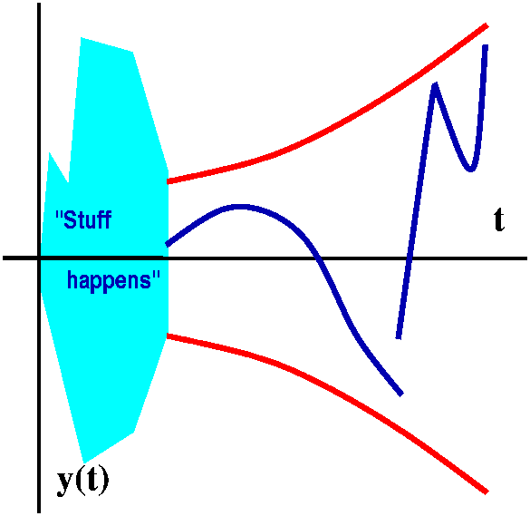
The classical Laplace transform works with functions that have growth
no bigger than exponential growth. This means that a function f(t)
must satisfy some sort of estimate of the following type:
There are positive constants A and B so that |y(t)|<AeBt
for t>C, where C is some additional positive constant.
There's sort of a picture of the situation to the right. The "Stuff
happens" doesn't sort of matter. What matters is that for t large
enough (t>C), y(t) is "trapped" between AeBt and
-AeBt. The two curves occur because there are absolute
value signs around the y(t). If y(t) is trapped that way, then in the
integral that defines the Laplace transform, 0infinitye-sty(t) dt,
when s>B, the integral is less than e(B-s)t in absolute
value, and since this is exponential decrease the integral must
converge.
t216,000/( .003e.000007t)
as
t-->infinity. Both the top and the bottom go to infinity. Use L'H lots
of times. If you use it 216,000 times, the result is
(Some huge constant)/[(Another stupid constant)e.000007t]
because the polynomial's powers go down to 0, and the bottom is still an exponential with positive exponent, and just "spits out" positive multiplicative constants upon differentiation. But the limit now, after 216,000 uses of L'H is 0, because the fraction is really just
CONSTANT/(exponential growth)
Therefore for large enough t, this is less than, say, 1.
tt=eln(t)·t.
Indeed, I agree: ln(t) can't be bounded by ANY POSITIVE CONSTANT,
so there's no B that will work.
Well, here in the board (I said, motioning to the side blackboard) is
a table of Laplace transforms. It turns out that it is also, more or
less, sort of, almost, also a table of inverse Laplace
transforms. Here in a wonderfully logical 640 subject course what
do the words "more or less, sort of, almost ..." mean?
If two functions have the same Laplace transform, then they differ only on a collection of values that the integral doesn't notice.
If F(s) is the Laplace transform of f(t), then the Laplace transform
of eatf(t) is F(s-a).
0infinitye-st+atf(t) dt
which is the same as 0infinitye-(s-a)tf(t) dt
and that is exactly the Laplace transform of f(t) evaluated at
s-a, or F(s-a).
Uhhh, can we find the Laplace transform of e5tsin(3t)? The
table stated that the transform of sin(3t) is 3/(s2+9). But
(take a=5) the Laplace transform of e5tsin(3t) must then be 3/((s-5)2+9).
More ofter we'll need to apply this result backwards. Can we find a
function whose Laplace transform is 5/(s+7)14? We look at
the table and see that this seemed to be Constant/s14
shifted. So this should be related to the Laplace transform of
t13. We needed to fix up the multiplicative constant so
that we would get 5. And therefore we multiply t13 by 5 and
divided it by 13! so that the Laplace transform of
(5/(13!)t13 is 5/s14. Now we need to shift by
-7, and conclude that the Laplace transform of
e-7t(5/(13!)t13 is 5/(s+7)14.
Isn't this cool!
I defined the Heaviside or unit step function, called
U(t) in your text (actually with a calligraphic U). Oliver
Heaviside was a brilliant English engineer whose life was,
overall, rather sad. U is the function which is 0 for t<0
and is 1 for t>=0. There's a jump of 1 at 0, and otherwise the
function's graph consists of two half lines.
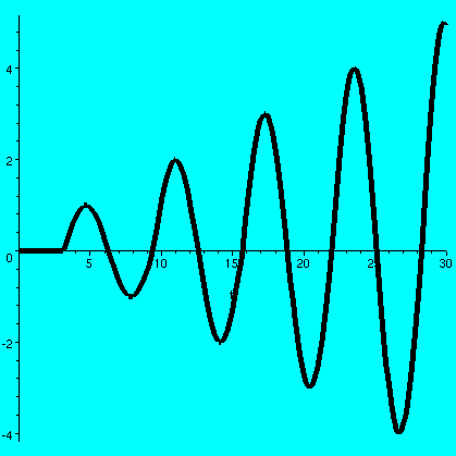
Using U
I think I graphed a few
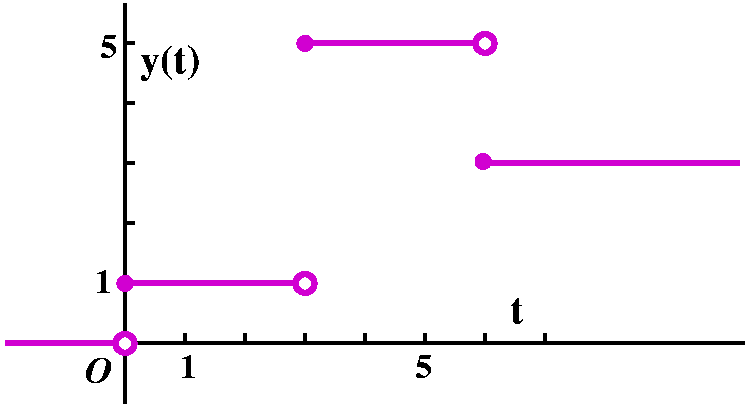
examples, like U(t-3) (the jump is moved to 3) and
U(t)+4U(t-3)-2U(t-6) (the graph "starts" at 0
with a jump up at 1, jumps up 4 (to 5) at 3, and then down 2 (to 3) at
t=6 - aside from the jumps the graph just is pieced together from
horizontal line segments.
U(t) allows us to write formulas for
other piecewise defined functions.
What's a formula for y(t)? I sort of work from left to right in t.
First there's nothing. Then we want to "turn on" t2 at t=0,
so we need t2U(t). Then we need to turn off t2
at t=1, and turn on a height of 1. Hey, change the formula to
t2U(t)+(-t2+1)U(t-1). Now let's continue to the
right, where we need to turn of the height of 1, and turn on the
downway parabolic arc. This change is (-1+(t-4)2)U(t-3) and
should be added to what we already had. Then, finally, at 4, turn off
(t-4)2 with -(t-4)2)U(t-4). So a formula for this function is
t2U(t)++(-t2+1)U(t-1)+
(-1+(t-4)2)U(t-3) -(t-4)2)U(t-4)
>y:=t->t^2*Heaviside(t)+(-t^2+1)*Heaviside(t-1)+(-1+(t-4)^2)*Heaviside(t-3) -(t-4)^2*Heaviside(t-4):
>plot(y(t), t=-1..6,thickness=3,scaling=constrained);
Now we are lost ...
This is all your fault. We are about 40% of a lecture behind. I think
I will begin on Thursday by remarking that you can easily catch up, so
I will begin where I should begin. Humph.
I retruned the Entrance Exam. I view this exam as a very useful
diagnostic, which has shown some correlation with final course grades
in Math 421. For me, it is useful because the exam shines a light on
two aspects of students. First, it clearly shows student knowledge of
representative content: everything asked on the exam will be
relevent to parts of the course, and, actually everything asked on the
exam is important in sections of the course. Second, given an
Entrance Exam like this to a group of somewhat sophisticated
educational "consumers" reveals a bit about their psychology: are they
willing to work, to review, to ask questions ... students who do these
things are more likely to learn, and not just barely survive. As I
mentioned in class, this is a fairly advanced undergraduate course,
and the person most resposible for teaching you is ... well, you! I
hope I will be helpful, but stuff will go by very rapidly. I strongly recommend working with one or more other
students in the course on a regular basis, meeting weekly or more
often for an hour or two. This is likely to keep you "on task", and
working together you will increase the odds of success.
My official office hours will be Busch period 4 on Monday and
Thursday, immediately after class. Since few of you are new college
students, you of course know that these times are first chosen to be
convenient for me. But, please, I will likely be in my office many
other times during the week. You can try to drop me. I may be busy,
but there's a good chance we'll be able to talk. Further I invite you
to make a mutually agreeable appointment with me. Probably the best
way to do this is by e-mail.
Confession
L(y1(t)+y2(t))=0infinitye-st[y1(t)+y2(t)] dt=0infinitye-st[y1(t)]+e-st[y2(t)] dt=0infinitye-sty1(t) dt+0infinitye-sty2(t) dt=L(y1(t))+L(y2(t)).
Similarly, if c is a constant, then L(cy(t))=cL(y(t)).
Linearity is a tremendously useful property, and we will use it
constantly.
In many of these computations, there will be plenty of minus signs and
much opportunity for error. I don't know how to avoid all errors.
One of great powers of the Laplace transform is its ability to deal
with rough functions: functions that may not be differentiable
or may not be continuous (or even, as we will see later, may not be
functions!). These rough functions are probably more accurate models
of many physical situations than the standard functions of calculus.
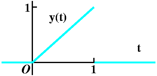
Here is an example. We will consider the piecewise-defined function
=0 for t<0
y(t)=t for t for t in [0,1]
=0 for t>1
A graph of this function is shown to the right. It certainly is not
continuous at t=1. We will compute its Laplace transform.
Strategic note You will do more computations using integration
by parts in this course than ever before during a similar period of
your life. (And maybe [likely!] during any similar period for the
remainder of your life!)
For integration by parts, I generally write all the details. I have
made too many mistakes and I've gotten
tired of fouling up. I usually write:
01e-stt dt=
u dv = uv] - v du
u= } { du=
dv= } { v=
Then I try to make a good choice for u and see what happens. Your
experience must guide you, but generally you want to "exchange" the
u dv integral for a "better" v du integral.
01e-stt dt=
-(t/s)e-st]01-01(-1/s)e-st dt
Now the "boundary term" (as the uv term is sometimes called) is
-(t/s)e-st]01 which contributes
-e-s/s to our result.
-01(-1/s)e-st dt can be
integrated directly and we get
-{-{-1/s2}}e-st]t=0t=1 and this is
-e-s/s2 (from t=1) -{-1/s2} (from
t=0).
The total result is
-e-s/s-e-s/s2+{1/s2} and, in one fraction, this is
(-se-s-e-s+1)/s2
It might be useful to have some simple things that can be checked
about Laplace transforms. Then we might be able to look for errors,
etc. Also, the asymptotic statements I'll make turn out to be what can
be observed. Frequently, for example, in chemical kinetics, we can
only see what happens for large values of the parameter -- things
change too quickly.
Suppose our y(t) is some sort of collection of lumps and bumps, sort
of as shown. Well, the Laplace transform formula multiplies this by
e-st, and integrates dt. We will only consider positive s,
so the exponential is always decreasing. When s gets larger and larger
positive, the exponential decreases more and more rapidly to 0. Yes,
it stays at 1 when t=0, but the dropoff gets very rapid indeed. The
product of the exponential with y(t) will be some collection
{l|b}umps, but the amplitude, the height, will surely -->0. So
for the functions we are considering, Y(s)-->0 as s-->infinity.
What about as s-->0+? Well, heck, you folks are engineering
students. I would first try "plugging in" s=0. The result is 0/0. I know what to try next: l'Hopital. So we d/ds the top and bottom of Y(s)
separately. The result is (if I do it correctly!)
(-e-s+se-s+e-s)/(2s). Now plug in
again. Hey, the result is ... uhhhh ... 0/0. You could use l'H again,
but in fact, if you clean up the fraction algebraically you'll
see that the result is e-s/2, and as s-->0+,
this certainly --> 1/2, the area of that little triangle region.
Diary entry in progress! More to
come.
two little triangles, change of variables
Diary entry in progress! More to
come.
infinitely many triangles (!)
Here is a major result which will help to answer "Why are we doing all
this?"
If F(s) is the Laplace transform of f(t),
what is the Laplace transform of f´(t)?
0infinitye-stf´(t) dt=e-stf(t)]0infinity-0infinity(-s e-stf(t) dt.
There is all sorts of sneaky stuff going on here, and we should be
very careful. Let's see. The boundary term is
e-stf(t)]0infinity. Now
s>0, so when t-->infinity, e-stf(t)-->0. Technically I
am using the fact that f(t) doesn't grow too fast (in fact, eventually
it is "killed" by exponentials decreasing fast enough, e-st
for large s), but let's just try to get the mood of this method. When
t=0, we get -f(0) since e0=1. What about the integral term?
Notice that there are two minus signs. They cancel. What's left
is s multiplied by the Laplace transform of f. So now we know:
Confession
Existence and Uniqueness Theorem for ODE's
Suppose f(t,y) is a differentiable function in both t and y for
(t,y)'s in a region in R2, and that the point
(t0,y0) is in the region. Then the ODE
y´=f(t,y) has a unique solution going through the point
(t0,y0).
Another way of writing the IC is y(t0)=y0.
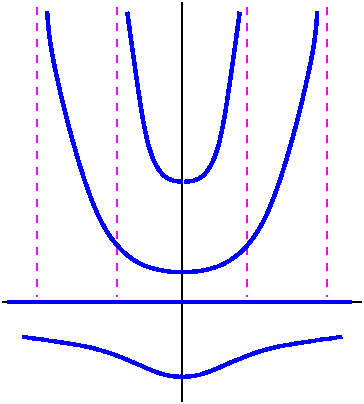
The picture to
the right is supposed to an impression of the geometry of the solution
curves to this ODE. Notice, please, that the Existence and Uniqueness
Theorem is totally correct, but really unhelpful. No inspection of
f(t,y)=ty2 seems to show anything wrong (!!) with the
function, but many of the solutions don't "live" very long, and they
live for different amounts of time.
The solutions blow up in the most immediate way
(y-->infinity) at different values of t. This ODE is nonlinear. We
will mostly concentrate on linear ODE's, where it turns out that such
problems don't occur.
This is very pleasant. If we go back momentarily to y´=ty2,
then look: even though 2/(.02-t) and 2/(.0002-t) are solutions, the sum,
2/(.02-t)+2/(.0002-t) is not a solution, and 22/(.02-t) is not a
solution. The linearity of the ODE is tremendously convenient. Linearity
has an elaborate classical name, the principle of
superposition. In mathspeak, the solutions of this homogeneous ODE
form a vector space. I would like to describe a convenient basis of
this vector space.
If y2 is a solution, then
y2´´+y2=0.
Add the equations to get
y1´´+y1+
y1´´+y1=0. Rearrange and recognize that this is
the same as
(y1+y2)´´+(y1+y2)=0, so
y1+y2 is a solution.
Multiply the equation by a
constant, C, to get
C(y1´´+y1)=0. Again, rearrange and recognize
that we have (Cy1)´´+(Cy1)=0, so Cy1
is a solution.
eit=cos(t)+i sin(t) and
cos(t)=[eit+e-it]/2
and
sin(t)=[eit-e-it]/(2i)
Part I of the course: Escaping the
wolves!
The snow was coming down thicker and the chill, at first merely
uncomfortable, was becoming a serious problem. With nightfall, we
could hear the howls of the wolves coming closer. It was time to try
for the Duke's castle and safety! I grabbed the child, and jumped on
my horse. I called to the others in the party, "Get on your brave
steeds, and ride rapidly to the castle ..."
Part I of the course: the Laplace transform
Remarks about the definition
Why should we study Laplace transforms?
Example 1 What is the Laplace transform of f(t)=1? We must
compute 0infinitye-stdt. I'll
work very slowly, with mathematical propriety:
0infinitye-stdt is the limit as
A-->infinity of
0Ae-stdt. Now we need an
antiderivative with respect to t of e-st. That's
-(1/s)e-st. Then we must evaluate
-(1/s)e-st]t=0t=A which is
-(1/s)e-sA-{-(1/s)}es·0.
I'm trying to go very slowly here, since it our first computation.
Now the exponential function's value at 0 is 1. And also the
exponential function dies off very quickly for negative real
arguments: the limit of ew is 0 as w-->-infinity, and, in
fact, it goes so rapidly to 0 that polynomial growth doesn't
stop it: w238ew-->0 as w-->-infinity also.
Since A>0,
-(1/s)e-sA-{-(1/s)}es·0=
-(1/s)e-sA+(1/s)-->1/s as A-->infinity.
Therefore the Laplace transform of 1 is 1/s.
which isn't much. I can think of several "patterns" which might extend
this table. So let us be a bit more patient, and compute the Laplace
transform of t2 directly from the definition:
0infinitye-sttdt. Again,
integration by parts works (we're going to do a great deal of
integration by parts, so get used to it!):
u=t2 so dv=e-stdt and du=2t dt and
v=-(1/s)e-st. The uv] term is
-(t2/s)e-st]t=0t=infinity
and this vanishes when t=0 surely, and as t-->infinity, since s>0
and exponential decay is faster than polynomial growth the
result is again 0. The remaining integral is (keep track of - signs!)
-e0infinty-st-(2t/s) dt. We pull
out the things which are constant relative to t, and get
(2/s)0infinitye-stt dt.
But the integral is the Laplace transform of t, which we already know
is 1/s2. Therefore we multiply this by 2/s to get the
Laplace transform of t<2.
If we look at the process, we see that if we want to get the Laplace
transform of t3 we will need to integrate by parts, and the
integration will "spit out" 3/s to multiply by 2/s3. Here
is where I hope a good physical scientist will "know" the Laplace
transform of nonnegative integer powers of t, and a mathematician will
attempt a proof by mathematical induction. In any case:
Here I wanted people to use the linearity of the Laplace
transform.
Please begin to read the chapter
in the book about Laplace transforms, and begin the problems. Do the
Entrance Exam, and have the result
of that ready to hand in next Thursday.