Math 251 diary, spring 2006
In reverse order: the most recent material is first.
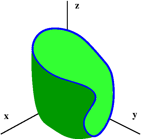
This is the fourth part of the diary: Vector calculus
A link to earlier material
Friday, April 28
[The last class: what sorrow, what
joy!]
Deriving the Heat Equation using the Divergence Theorem
I mostly followed the presentation here.
The heat equation governs a vast variety of propagation phenomena. I
know it is used to describe how heat distributes itself. It also is
used to analyze diffusion phenomena, such as salt in a solution of
water. It can be used, one colleague assures me, to study the
migration of moose. And how gossip spreads through a population. And
certain kinds of epidemics. And in finance, the heat equation applies
to analyze the flow (!) of money. The heat equation depends on two
fundamental assumptions. If "your" problem also can be translated so
it satisfies these two fundamental assumptions, then you also need the
heat equation. The names attached to what I'll describe here include
Newton, Euler, and Fourier.
We will deal with a homogeneous, isotropic material. Here
"homogeneous" means the material is the same from one point to the
next, and "isotropic" means that the directions around a point all
have similar properties. Bean soup is not homogeneous because of the
beans and the soup. A piece of
lumber is not isotropic because behavior with/against the grain is
different.
Assumption #1
The heat inside a small piece of material is directly proportional to
the mass of the material and the temperature. The constant of
proportionality is called specific heat. Using the language of
Math 251, we can write that the heat inside a small piece of
material= The pieceK(Density)u(x,y,z,t) dV.
Here K is the specific heat, and Density is the density of the
material (so Density dV is a small amount of mass). Density and K
are constants in our circumstances. u(x,y,z,t) is the temperature at
the point (x,y,z) of the material at time t. In class, and in the reference cited
above some specific heats are discussed (water has high K and
metals, lower).
The pieceK(Density)u(x,y,z,t) dV.
Here K is the specific heat, and Density is the density of the
material (so Density dV is a small amount of mass). Density and K
are constants in our circumstances. u(x,y,z,t) is the temperature at
the point (x,y,z) of the material at time t. In class, and in the reference cited
above some specific heats are discussed (water has high K and
metals, lower).
Assumption #2
Heat flows from hot to cold. The heat flow is directly proportional to
both the difference in temperature and to the cross-sectional area
through which the heat flows. If there is a big surface through which
the heat can flow, than there will be much more heat flow. And if the
temperature difference is high, there will be more heat flow. The
constant of proportionality here is called the conductivity,
c. Again, we discussed these assumptions in class and the reference
has further information. I can stir a hot stew safely with a wooden
spoon (relatively low conductivity) but I'd better be careful if I use
a spoon made of metal (higher conductivity).
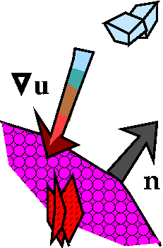
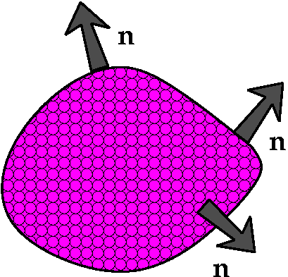
Hot inside
But I need to be careful. Consider a small part of the surface of our
small piece. Suppose, for example, that the inside of the piece is
warmer than the outside. The gradient of the
temperature,  u, points in the
direction of increasing temperature. So it will point towards the
inside of the piece. If we compare an outward-pointing unit normal,
then u·n will be negative because the
angle between the two vectors is between Pi/2 and Pi and cosine is
negative in that range. So if the inside is hotter,
u·n is negative.
u, points in the
direction of increasing temperature. So it will point towards the
inside of the piece. If we compare an outward-pointing unit normal,
then u·n will be negative because the
angle between the two vectors is between Pi/2 and Pi and cosine is
negative in that range. So if the inside is hotter,
u·n is negative.
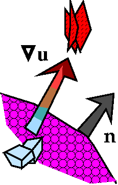 Hot outside
If the temperature is hotter outside, then the gradient vector of the
temperatur will point outwards, towards the higher temperature. Then
if we compute u·n the result will positive
because the angle between the two vectors is between 0 and Pi/2. So
the "contribution" of the dot product is positive if the outside is
hotter than the inside.
Hot outside
If the temperature is hotter outside, then the gradient vector of the
temperatur will point outwards, towards the higher temperature. Then
if we compute u·n the result will positive
because the angle between the two vectors is between 0 and Pi/2. So
the "contribution" of the dot product is positive if the outside is
hotter than the inside.
So the dot product u·n is positive when the heat flows
towards the piece and negative if the heat should flow away.
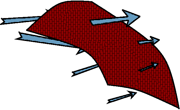
Art! By the
way, the pictures are supposed to show hot with flames and cold with
ice cubes. This is tremendously imaginative and wonderful. maybe
Therefore the amount of heat coming in/going out is The surface of the piececu·ndS.
But the change in the heat over time is also ( /t)The pieceK(Density)u(x,y,z,t) dV.
This is one place where our simplifying assumptions help a great
deal: K and the Density are constant. Only u varies with time. So
this is equal to
/t)The pieceK(Density)u(x,y,z,t) dV.
This is one place where our simplifying assumptions help a great
deal: K and the Density are constant. Only u varies with time. So
this is equal to
The pieceK(Density)(u/t) dV.
Now comes the magic! We apply the Divergence
Theorem to the surface integral giving the change in heat and get
The piecedivergence of cu dV.
Well, cu is
cuxi+cuyj+cuzk
and the divergence of this (c is a constant) is
c(uxx+uyy+uzz). By the way, the
collection of derivatives uxx+uyy+uzz
also has a specific name: it is called the Laplacian. Notation
for the Laplacian of u varies. In some places, 2u is used, and, otherwise,
 u is used.
And so:
We now know that for any little piece of the material, the following
triple integrals are equal because they both give the change in heat
of the little piece:
The pieceK(Density)(u/t) dV=The piecec(uxx+uyy+uzz) dV.
If we take a really really tiny piece, then the functions inside each
integral are approximately constant (because they are continuous!) so
we can approximate the integrals by the function values and the
volume:
K(Density)(u/t)The Volume=c(uxx+uyy+uzz)The Volume
Divide both sides by The Volume and get The Heat Equation:
K(Density)(u/t)=c(uxx+uyy+uzz)
Then we can "study" this equation: try to find approximate solutions
or to study qualitative aspects of solutions, or ... well, I will
admit it: only very rarely can exact solutions which are physically
interesting be found. It turns out that the heat equation and its
"solutions" are good models of many physical situations.
Another way to evaluate double integrals
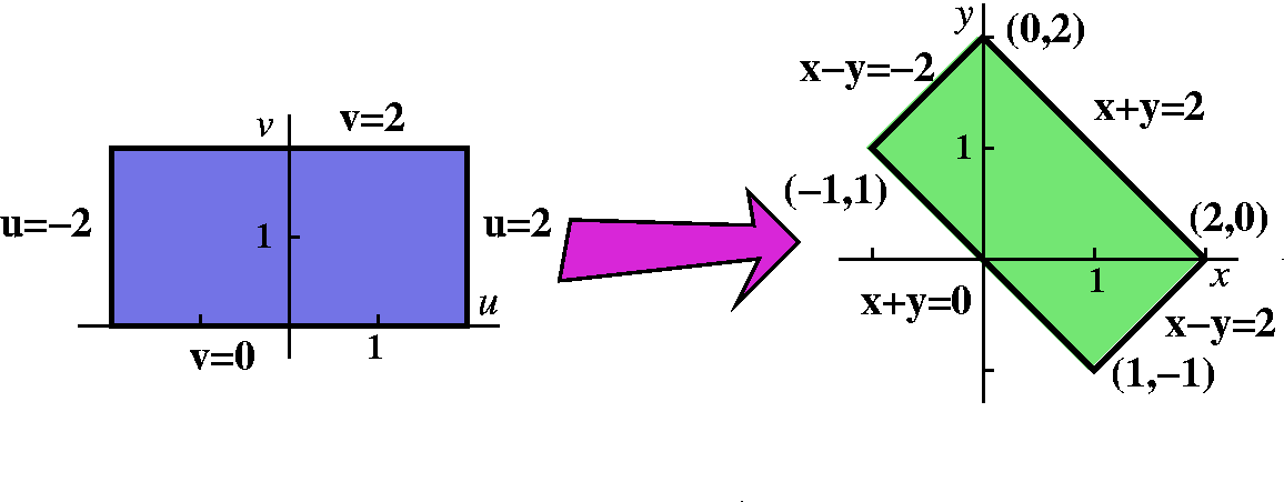
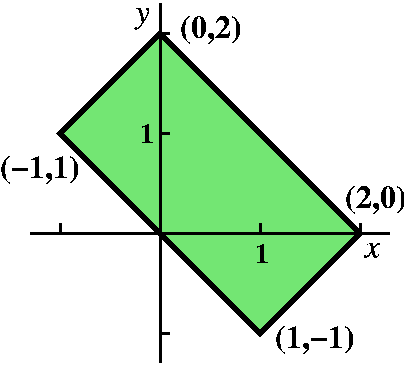 I began with the following example: compute
R(x-y)40(x+y)50dA where R is
the rectangular region with corners (1,-1), (2,0), (0,2), and (-1,1).
This is an irritating integral. But there is some not well concealed
symmetry. The boundaries of rectangle can be written as x+y=2,
x+y=0, x-y=-2, and x-y=2.
I began with the following example: compute
R(x-y)40(x+y)50dA where R is
the rectangular region with corners (1,-1), (2,0), (0,2), and (-1,1).
This is an irritating integral. But there is some not well concealed
symmetry. The boundaries of rectangle can be written as x+y=2,
x+y=0, x-y=-2, and x-y=2.
It almost seems as if the integrand and the region are begging
us to rewrite everything in terms of u and v where u=x-y and
v=x+y. Then the region of integration can be described -2<=u<=2
and 0<=v<=2. The integrand becomes
u40v50. Notice that if we add the equations
u=x-y and v=x+y and divide by 2 we get x=(1/2)(u+v). If we subtract
the first equation from the second and divide by 2 we get
y=(1/2)(v-u).
 We have parameterized the xy-plane by
r(u,v)=(1/2)(u+v)i+(1/2)(v-u)j+0k. There
is an area distortion factor which we computed as:
dAx,y=|ruxrv|dAu,v.
So let's compute:
We have parameterized the xy-plane by
r(u,v)=(1/2)(u+v)i+(1/2)(v-u)j+0k. There
is an area distortion factor which we computed as:
dAx,y=|ruxrv|dAu,v.
So let's compute:
ru=(1/2)i-(1/2)j+0k and
rv=(1/2)i+(1/2)j+0k and:
   (  i    j  k )
det( 1/2 -1/2 0 )=0i+0k+(1/2)k
   ( 1/2  1/2 0 )
Therefore:
v=0v=1u=-2u=2u40(x+y)50dA
becomes R(x-y)40v50(1/2)du dv.
This can be evaluated exactly easily:
(1/2)2·(241/41)(251/51).
What's going on?
If there is something common among the algebraic and geometric
specifications of a double (or a triple!) integral, then we can
sometimes take advantage. We can parameterize with
r(u,v)=x(u,v)i+y(u,v)j+0k. The functions
x(u,v) and y(u,v) are chosen (ideally!) so that description of the
region and the specifications of integrand are simpler. The "area
distortion factor", |ruxrv|, then turns out to
be the absolute value of the 2-by-2 determinant,
( x/u y/u )
( x/v y/v )
This is just the k
component of |ruxrv|: the i and
j components are 0 in this case. This determinant is called the
Jacobian.
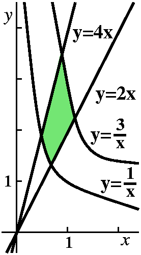 Another example
The following example could arise in thermodynamics or physical
chemistry. Suppose R is the region in the first quadrant bounded by
y=2x, y=4x, y=1/x, and y=3/x. Let's compute Rx4y dA.
Here a neat "change of variables" is a bit hidden, but maybe you can
see that the boundary curves of the region are y/x=2 and y/x=4 and
xy=1 and xy=3. Then you might (!) think to define u=y/x and v=xy. If
you do, then uv=(y/x)(xy)=y2 so that
y=u1/2v1/2. Then v=xy becomes
v=x(u1/2v1/2) so that
x=u-1/2v1/2. With the equations
x=u-1/2v1/2 and y=u1/2v1/2
the original integrand
x4y becomes u-3/2v5/2. The Jacobian
computation is:
( x/u y/u )  ( -(1/2)u-3/2v1/2   (1/2)u-1/2v1/2 )
( x/v y/v )  ( (1/2)u-1/2v-1/2   (1/2)u1/2v-1/2 )
and this is -(1/4)u-1-(1/4)u-1. We want
the absolute value (the magnitude of ruxrv) so we have
(1/2)(1/u). The double integral which results is
1324u-3/2v5/2(1/2)(1/u)du dv.
The region of integration has become a rectangle, the integrand is not
horrible, and the Jacobian factor is also not too bad.
I won't compute this, but I hope that you see it is easy enough.
This material is in section 15.9 of the text, Changing
Variables. It will not be tested on the final exam,
but you should see that the technique may be useful.
And so we end what one student in the class,
Ms. Karanam, called, perhaps appropriately, a course in

Tuesday, April 25
Problem R from the first set of review problems
Suppose that G(u,v) is a differentiable function of two
variables and that g(x,y)=G(x/y,y/x). Show
that xgx(x,y)+ygy(x,y)=0.
Solution Let's compute gx(x,y):
gx(x,y)=(/x)G(x/y,y/x)=(G/u)((x/y)/x)+(G/v)((y/x)/x)=(G/u)(1/y)+(G/v)(-y/x2).
And now gy(x,y):
gy(x,y)=(/y)G(x/y,y/x)=(G/u)((x/y)/y)+(G/v)((y/x)/y)=(G/u)(-x/y2)+(G/v)(1/x).
Both of these computations needed the Chain Rule in several
variables. Now we assemble
xgx(x,y)+ygy(x,y):
xgx(x,y)+ygy(x,y)=x[(G/u)(1/y)+(G/v)(-y/x2)]+y[(G/u)(-x/y2)+(G/v)(1/x)]=
(G/u)(x/y)+(G/v)(-y/x)+(G/u)(-x/y)+(G/v)(y/x)=0.
All the terms cancel.
Problem U from the first set of review problems
Suppose Q(x,y) is defined by the equation Q(x,y)=exf(y)
where f is a differentiable function of one variable with f(0)=A,
f´(0)=B, and f´´(0)=C. Use this information to compute these
quantities:
Q(0,0),
(Q/x)(0,0),
(Q/y)(0,0),
(2Q/x2)(0,0),
(2Q/xy)(0,0),
and
(2Q/y2)(0,0).
Solution Q(0,0)=e0f(0)=e0=1.
The other computations need the Chain Rule.
Q/x=(/x)exf(y)=exf(y)f(y), so
(Q/x)(0,0)=
e0f(0)f(0)=e0A=A.
Q/y=(/y)exf(y)=exf(y)xf´(y), so
(Q/y)(0,0)=
e0f(0)0·f´(0)=0.
2Q/x2=(/x)[exf(y)f(y)]=exf(y)f(y)2, so (2Q/x2)(0,0)=e0f(0)f(0)2=1·A2=A2.
2Q/xy=(/x)[exf(y)f(y)]=exf(y)xf(y)2+exf(y)f´(y), so
(2Q/xy)(0,0)=exf(y)xf(y)2+exf(y)f´(y)=e0f(0)0f(0)2+e0f(0)f´(0)=B.
2Q/y2=(/y)[exf(y)xf´(y)]=exf(y)x2f´(y)2+exf(y)xf´´(y), so
(2Q/y2)(0,0)=e0f(0)02f´(0)2+e0f(0)0f´´(0)=0.
[Not discussed in lecture.]
In the last three computations (the second derivatives) we use the
formulas for the first derivatives (before they are evaluated).
Statement of the Divergence Theorem
Suppose E is a solid bounded region in space (R3) and S is
the boundary of E, with n the outward pointing normal on
S. Suppose also that F is a vector field with differentiable
coefficients. Then:
SF·n dS=Ediv F dV.
The vector field, F(x,y,z), should be
P(x,y,z)i+Q(x,y,z)j+R(x,y,z)k and P, Q, and R
should be differentiable functions. The divergence of F is ·F: (P/x)+(Q/y)+(R/z).
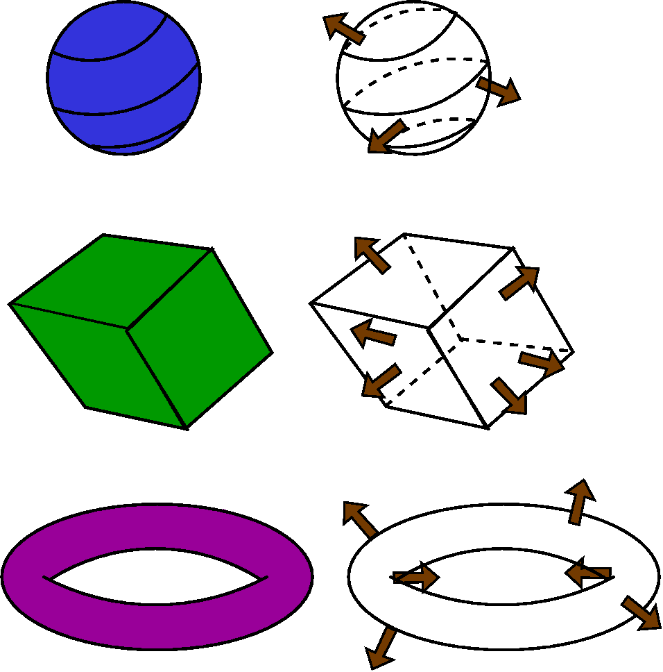
Simple examples of regions and surfaces
| Most "concrete" computations with the Divergence
Theorem will likely involve fairly simple shapes. |
- The sphere
Here the spatial region is the inside of a sphere (a ball). The
surface is the sphere, and the normals, a few of which are shown,
point outward from the center of the sphere.
- A parallelopiped
This is supposed to be an object with six flat sides, with the
opposite sides parallel in pairs. The surface has exactly 6 outward
normal vectors, one for each side.
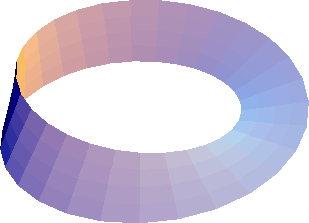
- A torus
The region in space is the region inside a torus. The surface has
normals pointing out, but now the surface is more complicated. Indeed
there are even some normals which point at each other!
|
|
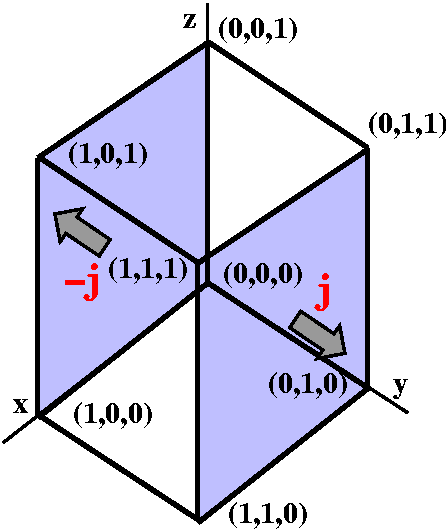
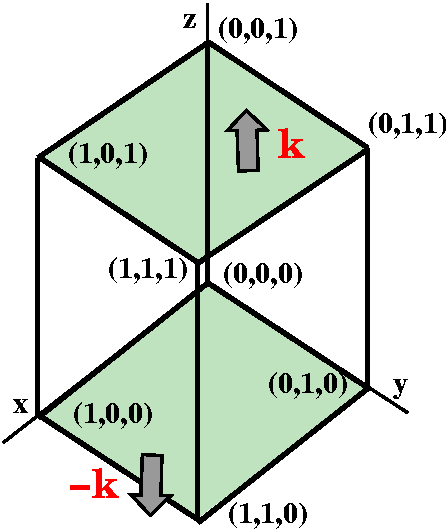
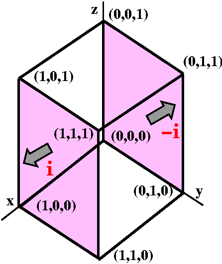
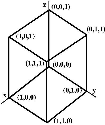 Proving the Divergence Theorem for the unit cube
I tried to "demystify" the Divergence Theorem by explaining why it is
true for the unit cube in R3.
The unit cube is a parallelopiped whose vertices (corners) have
entries 0 or 1. There are 8 vertices: (0,0,0), (1,0,0), (0,1,0),
(0,0,1), (1,1,0), (1,0,1), (0,1,1), and (1,1,1). There are 12
edges. Edges join at two vertices whose coordinates differ by one
entry. There are 6 faces, each obtained by holding one coordinate
equal either to 0 or to 1. By the way, the unit cube and its
generalizations in higher dimensions turn out to be very
interesting. One reason is the existence of Gray codes.
Now the triple integral side of the Divergence Theorem is
The cube(P/x)+(Q/y)+(R/z) dV. I will
split this into three separate integrals, and analyze each part.
 Let's look at The cube(Q/y) dV. I chose to write dV here as dy dAx,z. The reason for this is that the integration with respect to y will "undo" the
/y.
Let's look at The cube(Q/y) dV. I chose to write dV here as dy dAx,z. The reason for this is that the integration with respect to y will "undo" the
/y.
The innermost integral is then
y=0y=1(Q/y) dy. The Fundamental Theorem of Calculus immediately applies and we get Q(x,y,z)]y=0y=1=Q(x,1,z)-Q(x,0,z). We then integrate both of these:
x,z between 0&1Q(x,1,z) dAx,z-x,z between 0&1Q(x,0,z) dAx,z
Now look at the surface. The (x,1,z) part of the surface integral has
j as normal, and the (x,0-j
as normal. The surface integral of F·n will be -Q(x,0,z) and will be
+Q(x,1,z): both x and z will range from 0 to 1. The Fundamental
Theorem of Calculus yields a minus sign when "stuff" is at the lower
end of the integral. Geometrically, we get a minus sign on part of the
boundary because the normals are directed outward.
Let's look at The cube(R/z) dV. I would write dV as dz dAx,y. The
Fundamental Theorem of Calculus would apply to the innermost
integral:
z=0z=1(R/z) dz=Q(x,y,z)]z=0z=1=Q(x,y,1)-Q(x,y,0). Again
integrate both of these:
x,y between 0&1Q(x,y,1) dAx,y-x,y between 0&1Q(x,y,0) dAx,z
The minus sign comes from the Fundamental Theorem of Calculus and it comes from the +/-orientation of the normals.
Finally the last term is The cube(P/x) dV. I hope that you see dV here should be written as
dx dAy,z. Then the Fundamental Theorem of Calculus
applies and we've got this:
 x=0x=1(P/x) dx=P(x,y,z)]x=0x=1=P(1,y,z)-Q(1,y,z).
Each of these terms needs to be integrated with respect to y and z
from 0 to 1. The + part (that is, at
(1,y,z) in the cube) has a normal vector of i and the - part (that is, at (0,y,z) in the cube) has a
normal vector of -i. So this part of the triple integral, after
using the Fundamental Theorem of Calculus, gives the flux over the two
indicated pieces of the boundary of the cube.
If now we add up the three pieces of the triple integral we will get
the surface integral of F·n over
the boundary of the cube with the "correct" (outward) orientation. I
wanted to tell you that the Divergence Theorem is a version of the
Fundamental Theorem of Calculus, and that the signs checked out:
algebraically, they occur because of FTC and ]. Geometrically, they come from the
outward choices.
An old computation
We first introducted flux computations on April 18. And one of the examples given was this:
If F(x,y,z)= x2i+yzj-4zk, and
the surface is the sphere of radius 5 centered at the origin, what is
the total flux of F through this sphere (directed
outwards). Please look at what we did on April 18. We can also use the
Divergence Theorem:
The flux would be the (triple) integral over the whole sphere (its
inside!) of div F=((x2)/x)+((yz)/y)+((-4z)/z)=2x+z-4.
The integral of 2x over the whole sphere will be 0: there are
positive and negative chunks of the sphere which will
cancel. Similarly, the integral of z over the whole sphere will be 0
(the sphere is terrific, and has "balance" with respect to all of its
variables). by the way, the total integral of x33 and
y47 and z2003 over this sphere will be 0, for
the same reasons. I don't know what the integral of even powers would
be.
Therefore the flux is equal to the integral of -4 over the sphere. And
that's -4 multiplied by the volume of the sphere:
(4/3)Pi·53. The result is -(2000/3)Pi, that same
answer as we got from a direct computation. But I could use the
Divergence Theorem and symmetry/assymetry rather rapidly. So this is
good.
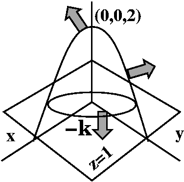 16.9, #20
Here is a standard textbook problem in the Divergence Theorem section.
F(x,y,z)=z arctan(y2)i+z3ln(x2+1)j+zk. Find
the flux of F across the part of the paraboloid
x2+y2+z=2 that lies above the plane z=1 and is
oriented upward.
Discussion and solution
The divergence of F is 0+0+1: we've gotten rid of a great deal
of mess! The paraboloid is z=2-x2-y2: it "opens"
down. The vertex or top is at (0,0,2). The normals to the paraboloid
vary a great deal. While it might be possible to compute the flux
directly, the Divergence Theorem states that the integral of 1 (that's
div F) over the solid region above z=1 and below
z=2-x2-y2 will equal the flux through the
parabolic cap plus the flux through the disc on the plane z=1. That
disc has radius 1, centered at the origin, since the boundary is
1=2-x2-y2 or x2+y2=1. Also
the outward normal on the disc is constant because the disc is flat,
and the outward normal is -k.
Let's compute the triple integral: The cup1 dV. Probably this is
simplest to compute with cylindrical coordinates.  will go from 0
to 2Pi, and r will go from 0 to 1. That's a polar description of the
base of the solid. What's the height? The bottom is at z=1, and the
top is at z=2-x2-y2, or (in "polar"),
z=2-r2. So we compute
will go from 0
to 2Pi, and r will go from 0 to 1. That's a polar description of the
base of the solid. What's the height? The bottom is at z=1, and the
top is at z=2-x2-y2, or (in "polar"),
z=2-r2. So we compute
=0=2Pir=0r=1z=1z=2-r21 dz r dr d==0=2Pir=0r=1(2-r2-1)r dr d=
=0=2Pir=0r=1(r-r3)dr d=
=0=2Pi(r2/2-r4/4)]r=0r=0d==0=2Pi(1/4)d=Pi/2.
Now the surface integral over the "bottom" disc. F·n is (z arctan(y2)i+z3ln(x2+1)j+zk)·(-k) which is -z. But z=1 on this disc, so we need to integrate -1 over a disc bounded by a circle of radius 1: the answer is -Pi.
We now have: Pi/2 (the divergence integral) equal to the flux over the
paraboloid plus -Pi (the flux over the disc). Therefore the flux over
the paraboloid must be (3Pi)/2.
Other uses
While textbook problems are (sometimes) nice, more interesting uses of
the Divergence Theorem include a discussion of heat transfer (Friday)
and maybe some mention of Gauss's Law. I tried to do Gauss's law and
screwed up in the lecture to sections 8, 9, and 10. Maybe I can do
better here.
Gauss's Law [Not discussed in lecture.]
Let's start with an inverse square force field in R3
centered at the origin:
F=-xi/(x2+y2+z2)3/2-yj/(x2+y2+z2)3/2-zk/(x2+y2+z2)3/2
I want the divergence of F so I probably need to compute things
like this: (/x)(-x/(x2+y2+z2)3/2)=I'm tired! I'll have a friend compute this:
> A:=diff(-x/(x^2+y^2+z^2)^(3/2),x):
> B:=diff(-y/(x^2+y^2+z^2)^(3/2),y):
> C:=diff(-z/(x^2+y^2+z^2)^(3/2),z):
> A+B+C;
                                             2       2       2
                                    3     3 x     3 y     3 z
                                - ----- + ----- + ----- + -----
                                    3/2     5/2     5/2     5/2
                                  %1      %1      %1      %1

                                             2    2    2
                                      %1 := x  + y  + z

> simplify(A+B+C);
                                               0
So the divergence of F is 0. But now let me compute the flux of
F across a sphere of radius A centered at the origin:
x2+y2+z2=A2. We can get a
normal to this sphere by taking the gradient:
2xi+2yj+2zk. A unit normal pointing "out" is
n=(x/A)i+(y/A)j+(z/A)k. Then F·n is
(-xi/(x2+y2+z2)3/2-yj/(x2+y2+z2)3/2-zk/(x2+y2+z2)3/2)·[(x/A)i+(y/A)j+(z/A)k]
Remember we're on the sphere
x2+y2+z2=A2 so this is:
(-xi/(A2)3/2-yj/(A2)3/2-zk/(A2)3/2)·[(x/A)i+(y/A)j+(z/A)k]=-(x2+y2+z2)/A4=-A2/A4=-1/A2
This should be integrated over the surface of the sphere. This is a
constant, so we just multiply the constant by the area of the sphere,
which is 4PiA2.
The flux is -1/A2(4PiA2)=-4Pi.
 Confusion!
But the divergence is 0 and the flux should be the integral of the
divergence, so ... what's going on? Again (we saw this earlier in an example with Green's Theorem) the vector field
F is not differentiable in all of the inside of the sphere: it
is not even defined at the origin. Here we have the flux equal to a
(non-zero) constant, not depending on the radius of the sphere.
Take any surface which completely surrounds the origin. Put a sphere
centered at the origin with very small radius between that surface and
the charge at the origin. The Divergence Theorem applies to the region
between the sphere and the origin since F is
differentiable away from the origin. But div F is 0 in
that region, so the total flux integral must be 0. That means
the flux integral outward through the surface is exactly balanced by
the flux integral inward through the sphere. The flux integral through
the sphere does not depend on the radius of the sphere, so the
surface flux doesn't depend on anything except that the surface
does wrap completely around the origin. And this is (a version of)
Gauss's Law: the flux integral around an isolated point charge is
always constant.
Gauss's Law is discussed in many physics books. Also you can look at
pages 1130 and 1131 of the textbook. Again, my apologies for messing
this up in lecture!
Friday, April 21
The remainder of the semester (hey: only 3 meetings!)
- Today: Stokes' Theorem, statement and discussion and examples
- Tuesday: The Divergence Theorem, statement and discussion and examples
- Next Friday: Change of variables, and the Heat Equation
Also I will discuss some review problems which had no answers sent to
me -- therefore they must be inaccessible and difficult and weird.
Today:
Problem Q from the second set of review problems
Sketch the three level curves of the function
W(x,y)=yex which pass through the points P=(0,2) and
Q=(2,0) and R=(1,-1). Label each curve with the
appropriate function value. Be sure that your drawing is clear and
unambiguous.
Also, sketch on the same axes the vectors of the gradient vector field
W at the points P and Q and R and
S and T. The point S=(0,-2) and the point T=(-2,0).
Problem solution and discussion
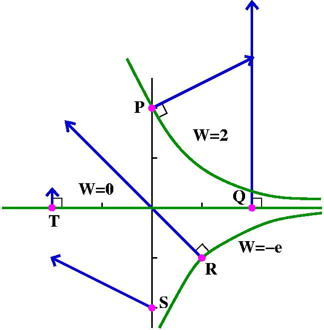 W(0,2)=2e0=2, so the level curve through P is
yex=2 or y=2e-x, an exponential decay.
W(0,2)=2e0=2, so the level curve through P is
yex=2 or y=2e-x, an exponential decay.
W(2,0)=0e2=0, so the level curve through Q is
yex=0 or y=0, a horizontal line.
W(1,-1)=-e1=-e, so the level curve through R is
yex=-e or y=-e1-x, sort of negative exponential
decay.
W=yexi+exj.
At P=(0,2), W=2i+1j.
At Q=(2,0), W=0i+e2j.
At R=(1,-1), W=-ei+ej.
At S=(0,-2), W=-2i+1j.
At T=(-2,0), W=0i+e-2j.
The drawing is shown, with level curves and points labeled. Please
note that the gradient vector field should always be perpendicular to
the level curves.
|
The ingredients for Stokes' Theorem
A simple closed curve
So this is a curve in space (R3) with START=END
and no other self-intersections.
|  |
A piece of surface
This should be a piece of a surface, all of whose boundary is the
curve mentioned above. As several students remarked, specifying the
boundary curve does not mean there's only one surface. In fact,
there are many really neat and clever computations which depend on
changing the surfaces involved. (We will do one of these below).
Work and flux
Stokes' Theorem involved computing the work of a vector field around
the closed curve, and then the flux of a related vector field over the
surface. So this means that we need to have a direction on the curve
(how we push things around) and we also need to make a selection of
normal vector on the surface. These choices need to be made together.
|  |
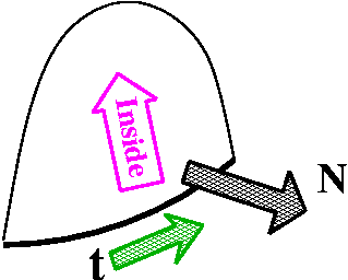
How the surface and curve interact (by their orientations)
The word "orientation" here means how to select t, the unit
tangent vector on the boundary curve, and N, the unit normal on
the surface. The boundary curve will be a parameterized curve. It has
a unit tangent vector, t, pointing in the direction of
increasing parameter value. If we "walk" along the boundary curve in
this direction, the surface should be to our left. Now we have
t and a direction to the left. Complete this to a right-handed
coordinate system. The selection of N, the unit normal vector
to the surface, is made so N points in the direction of the
last entry of the right-handed coordinate system. I think in the
accompanying picture to the right, the N would point "out" of
the page, and towards the "inside" of the cup-shaped surface.
| 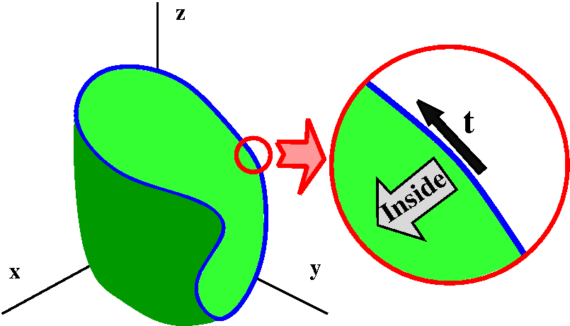 |
Under these conditions, then the Stokes Theorem Equation is
true:
The boundary curveF·t ds=The surfacecurl F·N dS
A textbook problem
 Here is problem 13 from section 16.7 of our textbook:
Verify that Stokes' Theorem is true for ... the vector field
F(x,y,z)=y2i+xj+z2k
and the surface is the part of the paraboloid
z=x2+y2 that lies below the plane z=1, oriented
upward.
Some discussion
The plane z=1 intersects the paraboloid in a circle. This is a circle
of radius 1 centered at (0,0,1). The paraboloid "overlays" a region
inside a circle of radius 1 centered at the origin in the xy-plane. We
will compute both integrals in Stokes' Theorem and (I hope!) get the
same answers. If the paraboloid is "oriented upward" then I presume
that the N points up. Going around the blue circle in the
standard (counterclockwise/positive) direction will orient the
boundary curve "compatibly": the t, the leftish piece of
surface next to the boundary curve, and the up N form a
right-handed triple.
The work integral
So I need to compute The curvey2dx+x dy+z2dz.
The curve is a circle, and can be parameterized as:
x=1cos(t) dx=-sin(t)dt
y=1sin(t) dy=cos(t)dt
z=1       dz=0
and the
parameterization interval for the whole circle is [0,2Pi]. Then The curvey2dx+x dy+z2dz
becomes
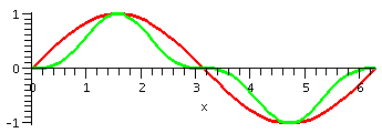
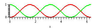
t=0t=2Pi-[sin(t)]3+[cos(t)]2dt.
I can "compute" this integral with tricks. It can also be
computed using the things done in Calc 2. But we're near the end of
the term, and tricks make the computations flow faster.
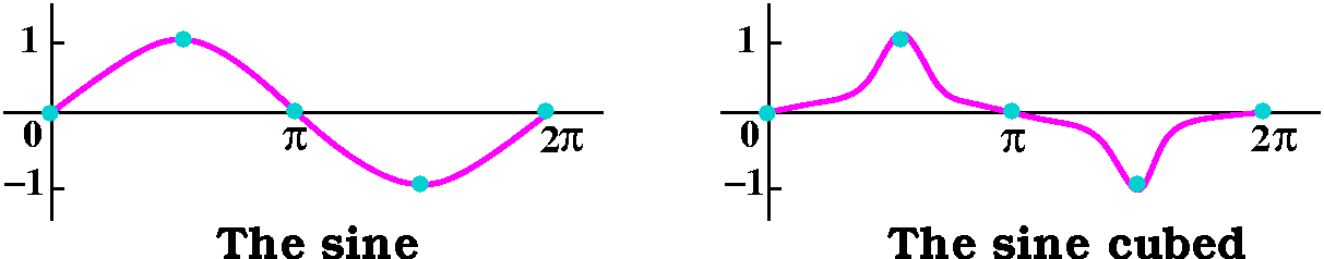
First, look at sine on the interval [0,Pi/2], and then look at
[sin(x)]3. Both the curves go up from 0 to 1. The
appearance is flipped left/right on [Pi/2,Pi], and then the appearance
on [0,Pi] is flipped down|up on [Pi,2Pi]. The total integral from 0 to
2Pi must be 0 because of the cancellation. The first picture below
shows my drawings of sine and the cube of sine. The red/green picture
with two curves shows a Maple graph of the two
curves. Consequence: t=0t=2Pi[sin(t)]3dt=0.
How about the integral of [cos(t)]2 on [0,2Pi]? The value
should certainly be the same as the integral of [sin(t)]2
on the same interval since the shapes are the same, just one quarter
period out of phase. The sum of these curves is 1
(sin2+cos2) which on [0,2Pi] has integral
2Pi. So t=0t=2Pi[cos(t)]2dt must be
half of that and it equals Pi.
The line integral side of Stokes' Theorem is Pi.
The surface integral
Now we need to compute The paraboloidcurl F·N dS.
The curl
This is xF, so:
   (  i     j    k   )
det( /x /y /z )=0i-0j+(1-2y)k
   (  y2    x     z2 )
Parameterizing the surface, etc.
Since the surface is presented as a graph, try the graph function
itself as a parameterization:
r(u,v)=ui+vj+(u2+v2)k so
ru(u,v)=1i+2ukand
rv(u,v)=1j+2vk.
Then ruxrv=
   ( i  j  k )
det( 1  0 2u )=-2ui-2vk+1k
   ( 0  1 2v )
We discussed the magical cancellation in the
last lecture. V·N dS became
V·(ruxrv) dAu,v.
curl F here is (1-2y)k=(1-2v)k so that
curl F·N dS=(1-2v)k·(-2ui-2vk+1k)dAu,v=(1-2v)dAu,v.
Computation of the surface integral
We need to identify the domain in the uv-plane which parameterizes our
little cup. The uv-plane is the xy-plane in different clothing, but
the cup is the graph over the region inside the unit circle:
u2+v2<=1. So we need
Inside the unit circle(1-2v)dAu,v
But the 2v integrates to 0, since the region is symmetric in v and 2v is "odd" (the + and - cancels totally). The 1 in the integrand just gives the area, and the area inside the unit circle is Pi(12), and this is Pi.
This instantiation (?) of Stokes' Theorem is verified: Pi=Pi.
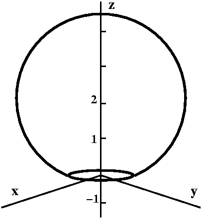 Another textbook problem
Here is a slightly more vicious (viscous?) problem from the Stokes'
Theorem section of a calculus text by Robert A. Adams:
Find The surfacecurl F·N dS where the surface is that part of
the sphere x2+y2+(z-2)2=8 which lies
above the xy-plane, and N is the outward unit normal on the
surface, and F is
y2cos(xz)i+x3eyzj-e-xyzk.
Since the problem occurs in the Stokes' Theorem section of the text we
should probably use Stokes' Theorem. The region of the sphere is shown
to the right. The sphere is centered at (0,0,2) and its radius is
sqrt(8)=2sqrt(2). So a portion of the sphere extends below the
xy-plane.
 The boundary of the top portion occurs if z=0 in the
equation
x2+y2+(z-2)2=8. Then
x2+y2+(-2)2=8 and
x2+y2=4. This is a circle of radius 2 centered
at the origin in the xy-plane. We should establish the orientation of
this circle. If we look closely at a small piece of the surface near
the boundary curve, the outward unit normal points slightly down. We
must "walk" along the curve so that the surface is to the left. The
t direction is the standard counterclockwise direction on the
boundary circle. I hope the local picture to the right helps to
convince you of that.
The boundary of the top portion occurs if z=0 in the
equation
x2+y2+(z-2)2=8. Then
x2+y2+(-2)2=8 and
x2+y2=4. This is a circle of radius 2 centered
at the origin in the xy-plane. We should establish the orientation of
this circle. If we look closely at a small piece of the surface near
the boundary curve, the outward unit normal points slightly down. We
must "walk" along the curve so that the surface is to the left. The
t direction is the standard counterclockwise direction on the
boundary circle. I hope the local picture to the right helps to
convince you of that.
Now Stokes' Theorem applies:
The spherical surfacecurl F·N dS=The boundary circleF·t ds.
 But notice: this circle is also the correctly oriented boundary of the
disc of radius 2 centered at the origin in the xy-plane. So I can use
Stokes' Theorem a second time to change the line integral to a
much simpler surface integral:
But notice: this circle is also the correctly oriented boundary of the
disc of radius 2 centered at the origin in the xy-plane. So I can use
Stokes' Theorem a second time to change the line integral to a
much simpler surface integral:
The boundary circleF·t ds=The disccurl F·N dS
This is simpler for several reasons. The region over which we're
integrating is flat, a disc in the xy-plane. The correctly oriented
normal, N, is just k. I hope the picture convinces you
of that.
We should compute curl F. Wait, we just need to compute
the k part of curl F:
    (     i       j      k   )
det (   /x    /y   /z )=Blah!i-Blah, blah!j+[3x2eyz-2ycos(xz)]k
    ( y2cos(xz) x3eyz -e-xyz  )
I further simplification occurs. We're on the xy-plane, where z=0. So
the k component [3x2eyz-2ycos(xz)] becomes
3x2-2y because cos(0)=1 and e0=1.
So we need The disc3x2-2y dAu,v. Just
as in the previous problem, the -2y integral over the disc is 0,
because there is cancellation of the positive and negative
contributions of y. I see no clever way to compute the 3x2
integral and will do this using polar coordinates (with
x=rcos()):
The disc3x2dAu,v=
=0=2Pir=0r=2r2[cos()]2r dr d=
3=0=2Pi[cos()]2dr=0r=2r3dr. The
integral is Pi (a trick used before) and the r integral is 16/4. So
the flux is 12Pi.
Comment I did this problem because using the same boundary
curve to switch surfaces is a very common "trick" done in
electromagnetism and fluid flow. If two surfaces have the same
boundary and if the vector field is nice, then the flux of the curls
of the vector fields through the two surfaces must be the same. This
is weird and wonderful, and people use it.
Green's Theorem [Not discussed in lecture.]
If the boundary curve is in R2 and the "surface" is a
region in R2 then Stokes' Theorem is Green's
Theorem. The only part of the curl that we see is the k, and if
the vector field is Pi+Qj+Rk, the normal N
is k and the k component of the curl of the vector field
is Qx-Py. So the integral of Pdx+Qdy over the
boundary curve (properly oriented) equals the double integral of
Qx-Py over the interior.
See page 1121 of the text.
What is curl?[Not discussed in
lecture.]
See page 1124 of the text. If F is a vector field, the text
shows how, using Stokes' Theorem, the vector curl F
represents how much the fluid flow
corresponding to F rotates.
Simply connected [Not discussed in
lecture.]
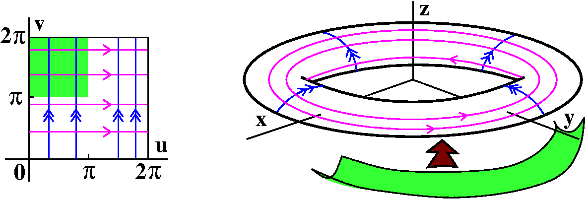
A region is simply connected if every simple closed curve can
be contracted to a point where the shrinking only occurs inside the
region. The picture below shows one simple closed curve shrinking to a point. In the torus, though, the red curve can't be shrunk to a point inside the torus.
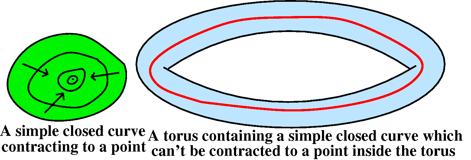
If a closed curve can be contracted to a point, and if F is a
vector field with curl F=0, then you can use Stokes'
Theorem to change the work integral around the curve to a flux
integral over a surface (the surface is green in the left-hand part of
the picture), and that integral is 0 since curl F=0. This
means in a simply connected region, any vector field whose curl is 0
must be conservative, and therefore must be a gradient vector
field. This doesn't necessarily happen in a non-simply connected
region, such as the torus. It turns out that such phenomena are
relevant to real-world applications.
This is on the bottom of page 1124 of the text.
Tuesday, April 18
Evaluations
You can evaluate the course, the instructor, and the penguin on
Friday, the next lecture.
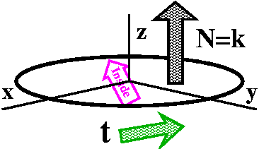
Coordinate charts
The picture and the understanding I wanted from the last lecture are:
a coordinate chart is a vector-valued function of two variables,
r(u,v). The u and the v live in some domain in R2,
and each pair (u,v) in that domain give (using ) a unique point on
the surface. Actually,
r(u,v)=x(u,v)i+y(u,v)j+z(u,v)k. is a
function with two inputs, u and v, and three outputs, x and y and
z. Dealing with a function like r abstractly can be
difficult. There are many variables and derivatives to keep track
of. In most cases that you're likely to encounter, the functions will
be related to some obvious geometry or other properties of the system
you're considering (look at the plane and sphere and torus from last
time). If v is constant and u varies, we get a curve on the surface in
R3. The velocity vector of that curve is
ru, the partial derivative of r with respect
to u. A similar thing is true about rv. The image of
a little u by v box in the uv-plane is a tiny
parallelogram (well, almost a parallelogram!) on the surface in
R3. The parallelogram is distorted by the velocity
vectors. The area of this parallelogram is |ruxrv|uV.
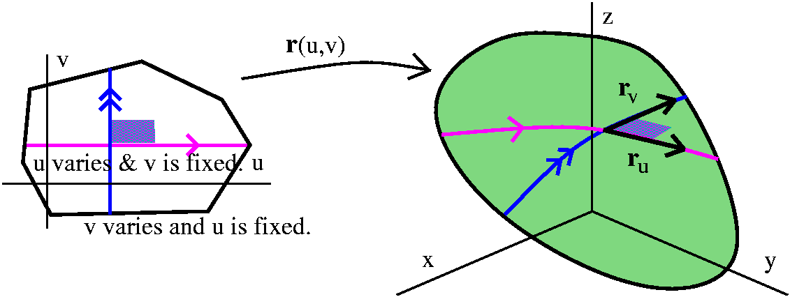
The advantage of (u,v) space is that things are easy to understand
there. On the surface itself, the coordinate curves need not be
orthogonal and the way they are put together can vary tremendously
from one point to the next.
dS
dS=|ruxrv|du dv.
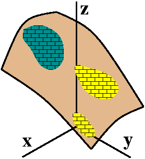 Surface integrals
If we believe a piece of surface in R3 could be a
mathematical model of a thin curved plate, then the plate could have
varying density. We could add up the density multiplied by the area to
get mass. This is a surface integral:
The SurfaceThe "density" function dS.
This will be computed using a coordinate chart, much as we computed
line integrals with parameterizations. Below are two textbook
problems. The picture to the right is supposed to be showing a thin
plate with ... uhhh ... some heavier and some lighter regions. As we
will see, this model doesn't correspond too well with the surface
integrals people actually compute, but, well, we can practice a bit
first.
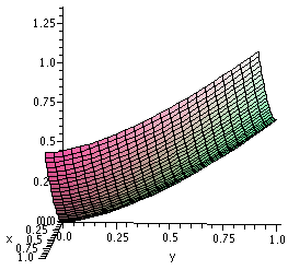 16.7, #8
Evaluate the surface integral.
The Surfacey dS,
S is the surface z=(2/3)(x3/2+y3/2), 0<=x<=1, 0<=y<=1
A picture of this textbook example is to the right.
The surface is a graph, and, for a graph, a first try at
parameterization would use the graph variables, and the graph
function:
x=u, y=v, and z=(2/3)(u3/2+v3/2) so
that
r(u,v)=ui+vj+(2/3)(u3/2+v3/2)k. We
can compute ruxrv:
   (  i   j    k  )
det(  1   0  u1/2  )=-u1/2i-v1/2j+k
   (  0   1  v1/2  )
The magnitude of this vector is sqrt(u+v+1). I hope that you realize the example
has been "invented" quite carefully so that the dS term is not very horrible. Imagine
if other powers had been used in the graph equation!
So dS=sqrt(u+v+1)dAuv where dAuv is just a piece
of (u,v) area. Since y=v, the integral The Surfacey dS in (u,v)-land is
v=0v=1u=0u=1v·sqrt(u+v+1) du dv.
Evaluating the integral
u=0u=1v·sqrt(u+v+1) du=(2/3)v(u+v+1)3/2]u=0u=1=(2/3)v(v+2)3/2-(2/3)v(v+1)3/2
because the integrand is just (integrating du!)
Constant1·sqrt(v+Constant2).
Now we need to antidifferentiate (dv) the function (2/3)v(v+2)3/2-(2/3)v(v+1)3/2. I'll do the first part:
(2/3)v(v+2)3/2dv=(2/3)(w-2)w3/2dw if the
substitution v+2=w, dv=dw, and v=w-2 is done. Then (2/3)(w-2)w3/2dw=(2/3)w5/2-(4/3)w3/2dw=
(4/21)w7/2-(8/15)w5/2=(4/21)(v+2)7/2-(8/15)(v+2)5/2. Then the definite integral (Maple tells me!) is
(12/35)sqrt(3)+(64/105)sqrt(2).
Students should try the other piece! You may check your answer:
the value of v=0v=1-(2/3)v(v+1)3/2dv is
reported to be -(8/105)-(16/35)sqrt(2).
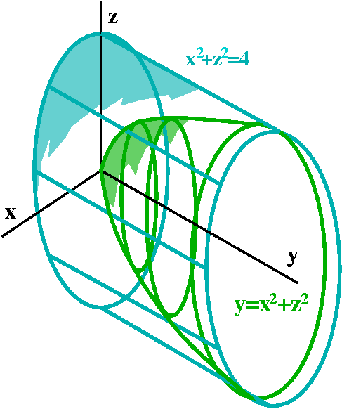 16.7, #11
Evaluate the surface integral.
The Surfacey dS,
S is the part of the paraboloid y=x2+z2 that lies inside the
cylinder x2+z2=4
In this case I decided to create a "hand" drawn picture since I
couldn't find an angle that I liked for a Maple graph. The
cylinder x2+z2=4 is a right circular cylinder
over a circle in the xz-plane. That circle has center at the origin
and radius 2. Then the cylindircal surface is gotten by pulling the
circle "out" parallel to the y-axis, which is the axis of symmetry of
the cylinder. The paraboloid y=x2+z2 also has
the y-axis as axis of symmetry. It "opens" out to the positive
y-axis. The cylinder and paraboloid intersect where y=4. The
paraboloid over which we will integrate is a graph over the inside of
the circle x2+z2=4 in the xz-plane.
Since the paraboloid is a graph, that suggests a parameterization:
x=u, y=u2+v2, and z=v, so that
r(u,v)=ui+(2/3)(u2+v2)j+vk.
And now ruxrv:
   (  i  j   k  )
det(  1   2u  0 )=2ui-1j+2vk
   (  0   2v  1 )
The magnitude of this vector is sqrt(4u2+4v2+1). y is
u2+v2. The surface integral we'd like to compute is
Inside (u,v) circle radius 2(u2+v2)sqrt(4u2+4v2+1) dAuv.
The computation
In this case, I hope that both the region of integration and the integrand suggest polar coordinates in the (u,v) plane. Then: dAuv=r dr d and the u2+v2 will be replaced by r2. The region of integration can be described in polar coordinates in a straightforward manner: goes from 2 to 2Pi and r goes from 0 to 2. So we need to compute:
=0=2Pir=0r=2r2sqrt(4r2+1) r dr d.
The most horrible thing in this antidifferentiation is
4r2+1, so I will try to compute the antiderivative of
r2sqrt(4r2+1) r with the substitution
w=4r2+1. This is a textbook problem, and things should
work! Also I see that I have a very helpful r along with dr. So:
r2sqrt(4r2+1) r dr=[(w-1)/4]sqrt(w)(1/8)dw since:
w=4r2+1. so dw=8r dr and (1/8)dw=r dr and
[(w-1)/4]=r2. I can compute this:
[(w-1)/4]sqrt(w)(1/8)dw= (1/32)[w3/2)-w1/2]dw=(1/80)w5/2-(1/48)w3/2=(1/80)(4r2+1)5/2-(1/48)(4r2+1)3/2. And now we need to substitute, etc. Or:
> int(int(r^2*sqrt(4*r^2+1)*r,r=0..2),theta=0..2*Pi);
                                                /         1/2   1/2       1/2\
                                            1/2 |  3128 Pi    17      8 Pi   |
                                          Pi    |- ---------------- - -------|
                                                ¥         15            15   /
                                        - ------------------------------------
                                                           32
> simplify(%);
                                                            1/2
                                                  Pi (391 17    + 1)
                                                  ------------------
                                                          60
Flux
The horrible factor |ruxrv| makes a "random" surface integral almost
impossible to compute in terms of antidifferentiations involving
familiar functions. It is very nice that the surface integrals of most
interest in physical and engineering problems are not "random" but
result from computations of flux, and it turns out that the horrible
factor disappears for such computations.
 Suppose we have a vector field, F in R3. We could
imagine a surface in R3, and then try to see how the flow
of the vector field interacts with the surface. The picture to the
right is quite imaginary. I've never seen the arrows of a vector
field, and I want the surface, sort of like a net, not to give any
resistance to the imaginary arrows. It is, of course, an imaginary
surface.
Suppose we have a vector field, F in R3. We could
imagine a surface in R3, and then try to see how the flow
of the vector field interacts with the surface. The picture to the
right is quite imaginary. I've never seen the arrows of a vector
field, and I want the surface, sort of like a net, not to give any
resistance to the imaginary arrows. It is, of course, an imaginary
surface.
The flux is the net flow through the surface.
What do the words mean?
net The direction the fluid flows means something. It is
possible that at some points the fluid crosses the surface in
different directions. We should have some way of giving a sign to the
flow, left to right/right to left, inward/outward, and then totaling
the different contributions, with signs, to see whether the net
flow is positive or negative.
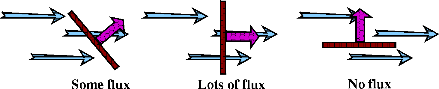 through The flow through the surface is important. The same
piece of surface ("dS") can have different flux, even if the vector
field is constant -- always the same direction and magnitude. What can
then change can be the angle of the dS piece relative to the flow. If
it is perpendicular to the flow, there will be the most flux. If the
dS is parallel to the flow, there will be no flux. In between,
there will be some "in between" amount. In fact, if you think about
this, the amount of flux will depend on the cosine of the angle the
surface makes with the vector field. We can compute this with
F·N where N is a unit vector
normal or perpendicular to the surface.
through The flow through the surface is important. The same
piece of surface ("dS") can have different flux, even if the vector
field is constant -- always the same direction and magnitude. What can
then change can be the angle of the dS piece relative to the flow. If
it is perpendicular to the flow, there will be the most flux. If the
dS is parallel to the flow, there will be no flux. In between,
there will be some "in between" amount. In fact, if you think about
this, the amount of flux will depend on the cosine of the angle the
surface makes with the vector field. We can compute this with
F·N where N is a unit vector
normal or perpendicular to the surface.
 The whole surface If we want to
compute the net flux through the whole surface, then we will need to
assign unit normal vectors at every point of the surface. There are
some surfaces which can't accept such assignments. The simplest
example is the Mobius strip (take a long rectangle, make a half-twist
in the long direction, and attach the short edges together). If you
give an N at any one point, and then follow around the
assignment continuously, when you get back to the point, you'll
discover that you have reversed the normal! So there will be no nice
way to define and compute flux through surfaces which don't permit
nice "assignments" of normals. I will assume such a problem will not
occur in the remainder of this course (hey, it doesn't for planes and
spheres and toruses and ... almost anything you will encounter in
applications).
The whole surface If we want to
compute the net flux through the whole surface, then we will need to
assign unit normal vectors at every point of the surface. There are
some surfaces which can't accept such assignments. The simplest
example is the Mobius strip (take a long rectangle, make a half-twist
in the long direction, and attach the short edges together). If you
give an N at any one point, and then follow around the
assignment continuously, when you get back to the point, you'll
discover that you have reversed the normal! So there will be no nice
way to define and compute flux through surfaces which don't permit
nice "assignments" of normals. I will assume such a problem will not
occur in the remainder of this course (hey, it doesn't for planes and
spheres and toruses and ... almost anything you will encounter in
applications).
Magical cancellation!
If our surface is parameterized there is a natural way to get a
unit normal. Just take ru and rv:
these are velocity vectors for curves on the surface, and are tangent
ot the surface. Their cross-product will be perpendicular to the
surface. If we then normalize (divide by the magnitude) we'll get an
acceptable N. So we can take N to be
ruxrv
divided by the scalar |ruxrv|. If Flux=The surfaceF·N dS this will be the same as
The surface[F·(ruxrv)/|ruxrv|] |ruxrv| dAuv
Look at the marvelous cancellation (much the same as what occurred in
the line integral case).
The flux integral is The surfaceF·(ruxrv) dAuv.
While a "plain" surface integral needs to be very carefully prepared
to be "computable" (as in the two previous examples), the cancellation
here means no horrible square root terms, and many flux integrals
should be computable.
An example on the sphere
Suppose F is x2i+yzj-4zk and I
would like to know the flux through the sphere of radius 5 centered at
the origin. We considered this surface before and
there we learned
ruxrv=-25cos(u)[sin(v)]2i-25sin(u)[sin(v)]2j-25sin(v)cos(v)k
and the parameterization itself was
x(u,v)=5cos(u)sin(v); y(u,v)=5sin(u)sin(v); z(u,v)=5cos(v). This means that F described in (u,v) terms becomes
25sin(u)2sin(v)2i+25sin(u)sin(v)cos(v)j-20cos(v)k
We need to integrate F·N dS, but
this, because of the cancellation of the horrible factor |ruxrv| becomes just F·(ruxrv) dAu,v. Let me match up the
components and get the integrand:
-625sin(u)2sin(v)4cos(u)-625
sin(u)2sin(v)3cos(v)+500cos(v)2sin(v).
This must be integrated from 0 to 2Pi in u and from 0 to Pi in v. I
emphasized in class that this integration is not difficult, even by
hand. You should at least vaguely remember integrating powers
of sines and cosines: they really weren't too hard. Maple
used about a tenth of a second of CPU time to tell me the value of
this double integral: -(2000/3)Pi. Next week, I'll show you how to get
the value of this flux integral using the Divergence Theorem with
practically no effort!
HOMEWORK
Read and do
problems in Chapter 16. Do problems! Do many problems!!
Friday, April 14
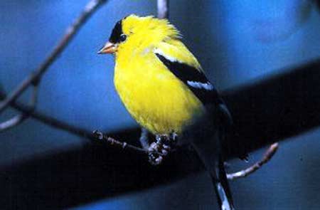 The state bird of New Jersey was in my backyard this morning. The
state bird of New Jersey is:
The state bird of New Jersey was in my backyard this morning. The
state bird of New Jersey is:
- The mosquito
- The bald eagle
- The corrupt politician
- The goldfinch
The answer is here.
The five integrals you meet in Math 251
Here's the list.
- One-dimensional integrals
13x2dx.
- Two-dimensional integrals
13xx3x2y5dA.
These can be rearranged, for example, in polar coordinates.
- Three-dimensional integrals
13xx3x+yx+y2x2y5z5dV.
And these also can be rearranged, for example, in spherical or
cylindrical coordinates.
- Line integrals
Cx2y3dx+zy2dy+xz2dz.
- Surface integrals
We will begin a discussion of parametric surfaces today, and then will
go on to considerations of surface area. We will meet surface
integrals themselves at the next lecture, Tuesday.
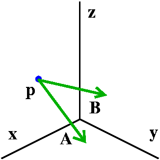
How to describe a plane
Suppose I give you a point, p=(3,1,2), and two vectors,
A=<4,-1,3> and B=<1,5,2>. I would like to
describe algebraically the plane which contains the point p in the
direction of the vectors A and B. Here is how we did
this problem earlier in the course.
An implicit description of the plane
Compute the cross-product of A and B:
   ( i   j  k )
det( 4  -1  3 )=-17i-5j+21k.
   ( 1   5  2 )
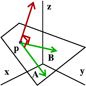 It is easy to check (I just did!) that the resulting vector is
perpendicular to both A and B and is a normal vector to
the plane we'd like to describe. A point with coordinates (x,y,z) is
on this plane if
It is easy to check (I just did!) that the resulting vector is
perpendicular to both A and B and is a normal vector to
the plane we'd like to describe. A point with coordinates (x,y,z) is
on this plane if
-17(x-3)-5(y-1)+21(z-2)=0.
This inplicit description, using a normal vector, was very convenient
for parts of the course since the gradient always gives a vector
normal to a level surface, and therefore normal to a tangent
plane. But there's another way to describe the plane.
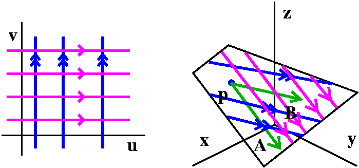
An explicit description
Change the point p=(3,1,2) to a position vector,
P=<3,1,2>. Then every point on this plane has a unique
description as P plus some multiple of A plus some
(possibly other) multiple of B. Your text calls these
multiplies u and v, so I will also. So the plane is anything which can
be written as P+uA+vB. We can write this with
more details:
<3,1,2>+u<4,-1,3>+v<1,5,2>=<3+4u+1v,1-u+5v,2+3u+2v>. The
textbook writes this as a vector position function:
r(u,v)=(3+4u+1v)i+(1-u+5v)j+(2+3u+2v)j
The i component is called x(u,v), the j component is
called y(u,v), and the k component is called z(u,v), Each point
on the plane has a unique "address" in terms of the pair of numbers
(u,v). This is like the central Manhattan street grid: streets and
avenues. So 3rd Avenue and 47th Street is a
unique point, and every intersection has a unique address.
 A sphere
Creating a "mapping" from a piece of the (u,v) plane to a surface in
R3 is frequently called a coordinate chart (although
not in your book). Getting a coordinate charts for a plane is not
difficult. Getting (useful!) coordinate charts for curved surfaces can
be much harder. Here's an example which is only moderately difficult
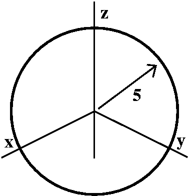
because we have studied spherical coordinates: a sphere of radius 5
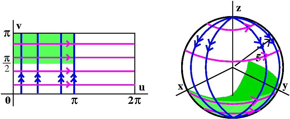
centered at the origin in R3.
Now let's use spherical coordinates, with rho fixed at 5. We see that
a point on the sphere will be described by (I use u for and v for phi):
x(u,v)=5cos(u)sin(v); y(u,v)=5sin(u)sin(v); z(u,v)=5cos(v).
I want points on the sphere to have unique (u,v) addresses, and the conventional choice for restriction of the (u,v) domain is 0<=u<=2Pi and 0<=v<=Pi.
Horizontal lines in the (u,v) domain become circles parallel to the
xy-plane on the sphere (latitudes?). Vertical lines in the (u,v)
domain, where v varies and u is fixed, become half great circles on
the sphere, going from the "North Pole" to the "South Pole". The
region in the (u,v) domain where 0<=u<=Pi and Pi/2<=v<=Pi
becomes the lower (z<=0) and "forward" (y>=0) quarter sphere.
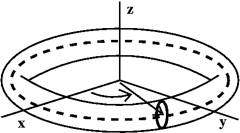 A torus
I'll try now to give a parametric description of a torus. So the torus
(the surface of a doughnut) will be a surface which is gotten when a
circle perpendicular to the xy-plane, and radially oriented, is
revolved around the z-axis. One view of what I'm trying to describe is to the right.
The center of the circle to be revolved around the z-axis is moved so that it describes a circle in the xy-plane centered at the origin. There are two more views below of the surface. One is from "above", looked down the z-axis. The other is from the "side", looking along the y-axis.
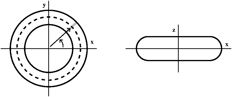
I can give points on the torus a unique "address" in terms of two
numbers. These two numbers will represent angles. One angle will be
, but I'll call it u to agree with the text.
I'll make this specific torus more definite: the length of the vector
from the z-axis to the center of the circle will be 4, and the radius
of the circle being revolved around the z-axis will be 2. The left
picture below shows the angle u. The right picture shows a slice
perpendicular to the xy-plane, through the vector of length 4. I will
specify a point on the torus by letting v be the angle made by a line
from the point on the torus to the center of the circle compared to
the xy-plane itself.
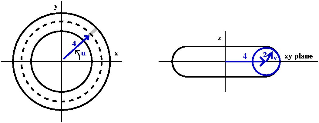
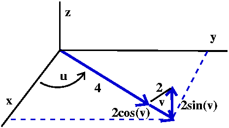 The z coordinate of the point only involves v. The z coordinate is the
"opposite" side of a right triangle with acute angle v and hypoteneuse
2. So z=2sin(v). The vector from the origin to the center of the
circle has length 4. The angle v adds on another 2cos(v) to that
length. But then we use this total length, 4=2cos(v), along with the
angle u (secretly, ) to get the x and y coordinates. So
x=(4+2cos(v))cos(u) and y=(4+2cos(v))sin(u).
The z coordinate of the point only involves v. The z coordinate is the
"opposite" side of a right triangle with acute angle v and hypoteneuse
2. So z=2sin(v). The vector from the origin to the center of the
circle has length 4. The angle v adds on another 2cos(v) to that
length. But then we use this total length, 4=2cos(v), along with the
angle u (secretly, ) to get the x and y coordinates. So
x=(4+2cos(v))cos(u) and y=(4+2cos(v))sin(u).
Therefore the torus will be given by the following vector-valued function:
r(u,v)=x(u,v)i+y(u,v)j+z(u,v)k with
x(u,v)=(4+2cos(v))cos(u) and
y(u,v)=(4+2cos(v))sin(u) and z(u,v)=2sin(v).
The domain of the coordinate chart, which will give each point on the
torus surface a unique (u,v) address, will be 0<=u<=2Pi and
0<=u<=2Pi.
In the 21st century I can check what I've just
written. Below is a Maple command and its output. I should
remark, if you've never been in my office watching me try to
use Maple, that typing this command and looking at its output
took 5 attempts before I was successful. Such wonderful effort may
explain why I wouldn't trust myself to use Maple in class
while people watched and giggled, and we all wasted time.
plot3d([4+2*cos(v))*cos(u),4+2*cos(v))*sin(u),2*sin(v)], u=0..2*Pi,v=0..2*Pi, scaling=constrained,axes=normal);
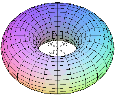
Finally, we can consider horizontal lines across the domain of the
coordinate chart, r(u,v), and ask what kinds of curves these
create on the torus. These lines, where u changes and v is unchanged,
become circles around the z-axis. Similarly, the vertical lines in the
domain of r become lines "around" the torus, for fixed u=.
If we restrict to region where 0<=u<=Pi and Pi<=v<=2Pi,
then the part of the torus which results is "forward" of the xz-plane
(where y>=0) and below the xy-plane (where z<=0). This is a
quarter of the torus.
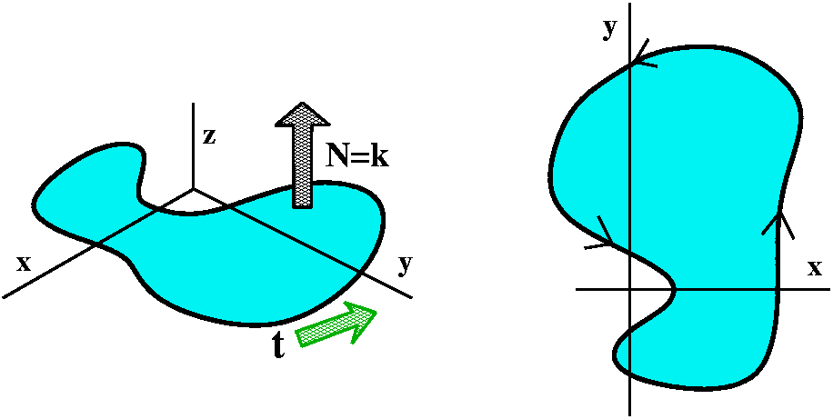
A graph
Here I considered a rather simple surface given by a graph:
z=3x2+5y4. Certainly all I expected people to
see and say was this this surface is (vaguely) cup-shaped, and its
lowest point is at (0,0,0). There's a really simple way to
parameterize such surfaces: just use x and y. So
r(u,v)=ui+vj+3u2+5v4k. The
parameterization geometrically consists of pushing up a grid from the
xy-plane until it hits the graph.
Surface area
Here once again was used the wonderful integral calculus slogan:
Cut up, approximate, sum, limit
This is very brief, since my eyes are tired! Please look in the
text for more details.
Small rectangles in the uv domain, of
dimension u by v were changed to approximate
parellelograms, and they were magnified by ru and
rv, respectively. The resulting area is obtained by
taking a cross product, and we get |ruxrv|uu. Then add these up and take the
limit. The surface area for a part of the surface which is
parameterized by a domain, D, in the uv-plane turns out to be
D|ruxrv| du dv. The
textbook calls |ruxrv| du dv by the
name, dS, for a piece of surface area.
The surface area of the sphere
Here
r(u,v)=5cos(u)sin(v)i+5sin(u)sin(v)j+5cos(v)k
Therefore
ru=-5sin(u)sin(v)i+5cos(u)sin(v)j+0k
and
rv=5cos(u)cos(v)i+5sin(u)cos(v)j-5sin(v)k
         (      i               j           k    )
ruxrv=det(-5sin(u)sin(v)  5cos(u)sin(v)     0    )
         ( 5cos(u)cos(v) 5sin(u)cos(v)  -5sin(v) )
The i component is just -25cos(u)[sin(v)]2 and the
j component is -25sin(u)[sin(v)]2 and the k
component is
-25[sin(u)]2sin(v)cos(v)-25[cos(u)]2sin(v)cos(v). The
last component simplifies (sin(u)2+cos(u)2=1) and the
result is
ruxrv=-25cos(u)[sin(v)]2i-25sin(u)[sin(v)]2j-25sin(v)cos(v)k
Now for the magnitude of this vector: the square root of the sum of
the squares of the components. There's a common factor of
252[sin(v)]2 when everything is squared, so I'll
take that out of the square root (sin(v) is positive when v is between
0 and Pi as it is here). So we must multiply 25sin(v) by
{cos(u)sin(v)]2+[sin(u)sin(v)]2+[cos(v)]2. Now
look at this: one use of sin(u)2+cos(u)2=1 turns
this into sin(v)2+cos(v)2 and that's 1 also! So
therefore we square root things and see that |ruxrv|=25sin(v). We get the whole sphere when the
coordinate patch is 0<=u<=2Pi and 0<=v<=pi, so the whole
surface area is 0Pi02Pi25sin(v) du dv. We
computed this integral and it was 100Pi. The surface area of a sphere
of radius r is supposed to be 4Pi r2 (four "great
circles") so when r=5 this is the textbook answer.
The surface area of the torus [Not discussed in lecture.]
You could try this yourself. The answer is 32Pi2, and a
detailed explanation is below.
Let's try this:
r(u,v)=(4+2cos(v))cos(u)i+(4+2cos(v))sin(u)j+2sin(v)k.
Then
ru=-(4+2cos(v))sin(u)i+(4+2cos(v))cos(u)j+0k
and
rv=(-2sin(v))cos(u)i+(-2sin(v))sin(u)j+2cos(v)k
         (          i               j               k   )
ruxrv=det(-(4+2cos(v))sin(u)  (4+2cos(v))cos(u)     0   )
         ( -2sin(v)cos(u)      -2sin(v)sin(u)   2cos(v) )
The i component is
8cos(v)cos(u)+4cos(v)2cos(u)=4cos(v)(2cos(u)+cos(v)cos(u)). This
is 4cos(v)cos(u)(2+cos(v)).
The j component is
8cos(v)sin(u)+4[cos(v)]2sin(u)=4cos(v)(2sin(u)+cos(v)sin(u)). This
is 4cos(v)sin(u)(2+cos(v)).
The k component is
8[sin(u)]2sin(v)+4[sin(u)]2cos(v)sin(v)+8sin(v)[cos(u)]2+4[cos(u)]2sin(v)cos(v). This
simplifies (again with sin2+cos2) to
8sin(v)+4sin(v)cos(v)=4sin(v)(2+cos(v)).
I have never done this computation before, but I hope it will work out. Now let us square and add the components:
42cos(v)2cos(u)2(2+cos(v))2+
42cos(v)2sin(u)2(2+cos(v))2+
42sin(v)2(2+cos(v))2
Again sin2+cos2 as indicated, and we get:
42cos(v)2(2+cos(v))2+
42sin(v)2(2+cos(v))2
One last time, sin2+cos2, and this becomes:
42(2+cos(v))2
This is |ruxrv|2, so we take the square root and
get 4(2+cos(v)) (notice that 2+cos(v) is always non-negative so the
square of its square is itself). Now to get the area of the whole
torus we need to integrate this over the uv-square which is [0,2Pi] by
[0,2Pi]. So the area is 02Pi02Pi4(2+cos(v)) du dv. The
answer is 32Pi2.
This answer is correct. A torus is such a symmetric figure that
its surface area can be determined using a (sort of) calculus-free
method called the Theorem
of Pappus.
The surface area of a piece of the graph
Here the integral turns out to be 0101sqrt(1+36x2+400y6) dx dy. Maple
can't "do" this integral, and gives the approximate value 6.8005 when
asked. Most surface areas can't be computed explicitely in terms of values of familiar functions.
Wednesday, April 12
I asked the beloved recitation instructors to return the exams and
give some basic statistics (see here
for further information). I also asked them to try to cover material
in 16.5. I hope that you saw something like this:
Vector fields in R3
Some simple examples of a three-dimensional vector
field. Again, fluid flows and force fields are examples.
If F=x2i+yj+yzk, compute the work done
along the twisted cubic x=t, y=t2, z=t3 for t
going from 0 to 1. What's this? Well, dx=dt and dy=2t dt and
dz=3t2 dt, so that
Twisted cubicx2dx+y dy+yz dz=t=0t=1(
t2+(t2)2t+(t2)(t3)3t2)dt=
t2+2t33t7dt=(1/2)+(2/4)+(3/8).
Now with the same vector field, the work done along a straight line
segment from (0,0,0) to (1,1,1). So one parameterization is x=t and
y=t and z=t with dx=dt and dy=dt and dz=dt. Then
Line segmentx2dx+y dy+yz dz=t=0t=1t2+t+t2dt=
2t2+t dt=(2/3)+(1/2).
The results are not the same, so we can again look for path
independence. A vector field is conservative if it is a gradient vector field. If P(x,y,z)i+Q(x,y,z)j+R(x,y,z)k has a potential f(x,y,z), then
fx=P and fy=Q and fz=R.
If there is a potential, then (just as in two dimensions and
for exactly the same reasons (the chain rule!) a line integral can be
evaluated with this simple idea:
CP(x,y,z)i+Q(x,y,z)j+R(x,y,z)k=Potential evaluated at the END of C-Potential evaluated at the START of C.
Getting a potential from a conservative vector field
You can try to find a potential by integrating in each variable
separately and comparing the resulting candidate descriptions of
f(x,y,z). Here is an example.
We will consider:
[2x·cos(2y)+3x2]i+[2x·cos(2y)+3x2]j+[-2x2sin(2y)+3y2e3z]k.
The coefficients of i and j and k will be called
P and Q and R, respectively, all functions of x and y and z.
- If P(x,y,z)=2x·cos(2y)+3x2 and if there is a potential
f(x,y,z), then since f/x should be equal to P, we know
that
2x·cos(2y)+3x2dx=x2cos(2y)+x3+C1(y,z).
- If Q(x,y,z)=-2x2sin(2y)+3y2e3z and if
there is a potential f(x,y,z), then since f/y should be equal to Q, we know that
-2x2sin(2y)+3y2e3zdy=x2cos(2y)+y2e3z+C2(x,z).
- If R(x,y,z)=3y3e3z-7 and if there is a
potential f(x,y,z), then since f/z should be equal to
R, we know that
3y3e3z-7 dz=y3e3-7z+C3(x,y).
Now we need to "reconcile" the three descriptions of
f(x,y,z). C1(y,z) is an appropriate "constant of
integration": here, any function of y and z. Similar remarks are true
for C2(x,z) and C3(x,y).
So f(x,y,z)=x2cos(2y)+x3+C1(y,z)
and
f(x,y,z)=x2cos(2y)+y2e3z+C2(x,z)
and f(x,y,z)=y3e3z-7z+C3(x,y).
If I look through these three descriptions, I can see where each piece
is "hiding" in each description and I can detect an f(x,y,z) which has
all of the desired features:
f(x,y,z)=x2cos(2y)+x3+y2e3z-7z.
Most important, look back: this formula satisfies all of the three
descriptions.
A quick way to check that there can't
be a potential is to consider the compatibility
conditions which follow.
Compatibility conditions
If P(x,y,z)i+Q(x,y,z)j+R(x,y,z)k is a gradient vector field, then
Py=Qx and Pz=Rx
and Qz=Ry
as a consequence of Clairaut's Theorem (equality of mixed partials)
applied to the mixed partials (the second derivatives) of the
potential function. To me this says that being a gradient vector field
is more difficult in 3 dimensions than in 2. In 2 dimensions there's
only one compatibility condition. In 3 dimensions there are 3. Things
only get worse as the dimensions increase. In classical physics,
describing the dynamics of just one particle means giving the position
(3 numbers) and the momentum (3 more numbers): you're already in
R6.
In R6 there are 6·5/2=15 equations required for the
compatibility conditions. So ... a gradient vector field there is
really rare.
Some notation which many people think is helpful
The conditions Py=Qx and
Pz=Rx and Qz=Ry may be
difficult to remember. Some new notation which is supposed to help
follows. Here is a quote from a web page entitled Earliest Uses of
Symbols of Calculus:
| The vector
differential operator, now written as an upside-down delta and called
nabla or del, was introduced by William Rowan Hamilton
(1805-1865). |
So "del" is given by: =(/x)i+(/y)j+(/z)k. Here are some uses:
- The gradient
We already know that if f(x,y,z) is a scalar function, then f is
fxi+fjj+fzk is
the gradient of f. This is a vector field.
- The curl
If F(x,y,z)=P(x,y,z)i+Q(x,y,z)j+R(x,y,z)k,
then the curl of F is another vector field, xF. It is a cross-product, and can be
evaluated by taking the determinant:
    (     i         j        k   )
det (   /x     /y     /z  )
    ( P(x,y,z) Q(x,y,z) R(x,y,z) )
It turns out this is equal to (if I don't foul up the signs!) the
following vector field:
(Ry-Qz)i-(Rx-Pz)j+(Qx-Py)k.
F satisfies the compatibility conditions above if
curl F=xF is 0. This isn't an accident. Hamilton
invented the del so that it would be useful!
- The divergence
If F(x,y,z)=P(x,y,z)i+Q(x,y,z)j+R(x,y,z)k,
then the divergence of F is a scalar function,
div F, defined by ·F. Written out in
more detail, div F is
Px+Qy+Rz.
The curl of a vector field is supposed to give some measure of how a
fluid flow modeled by the vector field curls "infinitesimally" around
each axis (x and y and z) at a point. The divergence of a vector field
is supposed to show for a fluid flow what the source or sink rate of
this flow is at a point. I will try later in the course to give more
information about this but I don't know if I will have time. A good
readable reference for students is the paperback previously recommended, Div, Grad,
Curl, and All That: An Informal Text on Vector Calculus, by
H. M. Schley which "I especially recommend for students
interested in physics and in mechanical or chemical engineering."
(That's just me quoting me.)
Here is a version of the big picture, sort of.
        =gradient           (x)=curl          (·)=div
Functions become Vector fields become Vector fields become Functions
Some examples computed
So start with f(x,y,z)=xy2z3. Then f=y2z3i+2xyz3j+3xy2z2k.
Let's take this vector field and compute its curl: ( i j k )
det ( /x /y /z )
( y2z3 2xyz3 3xy2z2 )
I think that the i component is (/y)(3xy2z2)-(/z)(2xyz3)=6xyz2-2xy(3z2)=0. The
other components are also 0 because of Clairaut! So
curl(grad of anything) is 0. Some people call vector fields
whose curl is 0 irrotational.
A gradient vector field is always irrotational.
Let me try another vector field:
F=y2zi+x2yzj+x3zk. The first component of the curl of F is (/y)(x3z)-(/z)(x2yz)=0-x2y=-x2y.
But please look at this:
> with(VectorCalculus):
> SetCoordinates('cartesian'[x,y,z]);
                                    cartesian[x, y, z]
> F:=VectorField();
                                  2   _     2     _     3   _
                            F := y  z e  + x  y z e  + x  z e
                                       x           y         z
> Curl(F);
                      2   _      2      2    _                      _
                    -x  y e  + (y  - 3 x  z) e  + (2 x y z - 2 y z) e
                           x                  y                      z
I did not know (but I suspected!) that Maple had a
curl command. I typed help(curl) and learned just a little about the
command. So the curl of our F is a vector field I will call
G, and G is
-x2yi+(y2-3x2z)j+(2xyz-2yz)k.
I'll compute the divergence of G. This div G is a
function, a scalar function. It is (/x)(-x2y)+(/y)(y2-3x2z)+(/x)(2xyz-2yz)=(-2xy)+(2y)+(2xy-2y)=0. The divergence of a curl
is always equal to 0: div(curl of anything)=0. If the
divergence of a vector field is 0, it is called
incompressible. So the curl of a vector field is
incompressible.
The vector field x2i+yj+z3k
has divergence equal to 2x+1+3z2, so it is not
incompressible.
HOMEWORK
Read on in
chapter 16. The next lecture will be about parametric surfaces (15.6)
and surface area (16.6).
Tuesday, April 11
Unfortunate event
I have had a detached retina which has been surgically
repaired. Convalescence from this has made me work at approximately 50%
efficiency. Consequences for the course include:
Return of graded exams has been delayed. I strongly prefer to
return exams as soon as possible. I also know that Friday may well be
a religious holiday for many people. Exams will be returned in
recitations tomorrow, April 12, along with solutions. At that time the
usual material relating to exams will be posted on the web.
I don't actually outsource writing the diary to Tibet, India, or
Nebraska. I do it myself, and each entry takes about 3 to 5
hours. Since I am working quite a bit more slowly now, I will probably
trim diary entries a good deal. The diary will become more of an
outline and have much less detail. Please attend class and take
notes.
The chemical of the day is Sulfur Hexafluoride. It seems to be colored dark
blue and I have a bubble of it in my eye. How interesting?
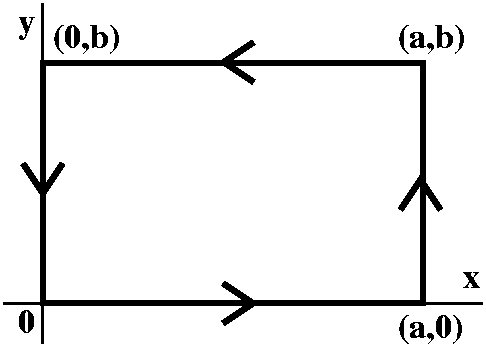 Rectangular Green's Theorem
During the last lecture (which may feel as if it were given a century
ago, due to the intervention of an exam), I verified a result called
Green's Theorem for a rectangle with corners at (0,0), (a,0),
(a,b), and (0,b).The verification amounted to some juggling with the
Fundamental Theorem of Calculus. The result was the following:
Rectangular bdryP(x,y)dx+Q(x,y)dy=Inside of rectQ(x,y)/x-P(x,y)/y dA.
Silly example
I first tried a rather silly example which was something like the
following. I think I took a=3 and b=2, and specified that
P(x,y)=5y+Junk1(x) and
Q(x,y)=x2+Junk1(y). Here the
Junk functions were some absurd formulas:
arctan(y3) or ecos(x). I wanted to compute the
line integral of P(x,y)dx+Q(x,y)dy around the boundary of the
rectangle. Of course I used the version of Green's Theorem stated
above, and the two Junk terms disappeared after the partial
differentiations, and the double integral had integrand 2x-5, which is
rather simple to compute over a rectangle.
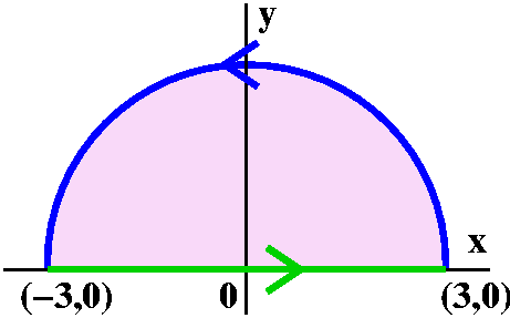 Computation on a semicircle
This is another example created for the classroom, but it is more
complex, and more resembles some real uses of Green's Theorem. Here I
considered the line integral Sy dx+x2dy
where S represents the upper half of the
circle of radius 3 centered at the origin. I think this integral
certainly can be computed straightforwardly by a parameterization but
I'd like to show another technique. First, what is the value of Ly dx+x2dy where L is the line segment along the x-axis stretching
from (-3,0) to (3,0)? Since y doesn't change on L, dy=0. Also notice that y=0 on all of L. Therefore y dx+x2dy is 0 on all
of L.
So Sy dx+x2dy=Sy dx+x2dy+Ly dx+x2dy=S+Ly dx+x2dy, and the
curve S+L, which is S
followed by L, encloses the upper half
of the area inside a circle of radius 3 centered at the origin: a
semidisc. I'll call it Q.
Then a version of Green's Theorem allows us to replace S+Ly dx+x2dy by Q(x2)/x-y/y dA. The
integrand is 2x-1, and we need to integrate it over Q.
The integral Q2x dA is actually 0, because
the region Q is symmetric with
respect to the y-axis, and 2x takes equally positive and negative
values on this region. So the values cancel each other. And the integral
Q-1 dA is minus one-half the area of a circle of radius 3. Therefore the original line integral,
Sy dx+x2dy, has the
value -9Pi/2.
I would agree that this is an awkward, even ludicrous way of
evaluating the line integral. I went through it because in a week
we'll be trying computations like this in three dimensions and maybe
things there won't be as clear.
The text's version of Green's Theorem
Suppose C is a positively oriented piecewise smooth simple closed
curve, and D is the region bounded by C. Suppose that P(x,y) and
Q(x,y) are functions with continuous first partial derivatives in
D. Then:
CP(x,y)dx+Q(x,y)dy=DQ(x,y)/x-P(x,y)/y dA.
Definitions of terms
The statement above is complicated, and I think many of the words need
some explanation.
- Closed curve
We have encountered this phrase before. A closed curve is a
parameterized curve which has an initial point (START) equal
to its terminal point (END).
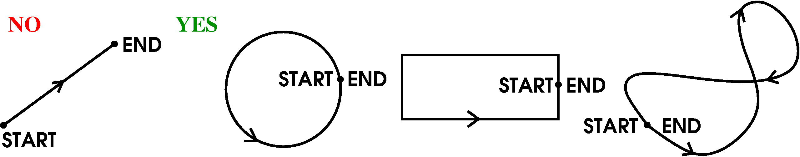
- Simple closed curve
A simple closed curve is a curve with no self-intersections
(crossings) except for the START=END.
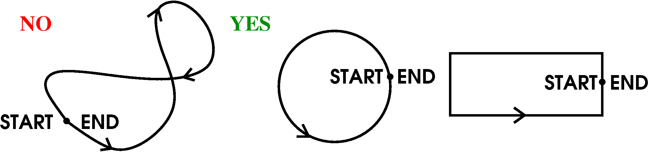
 One additional remark, please: simple closed curves don't have to be
so "simple" in the non-technical meaning of the word. I sketched
something like what is shown to the right. It may not even be clear
whether the point indicated in magenta (purple?) is inside or outside
the curve. So things can really get complicated if you want to do curves more complicated than circles or rectangles.
One additional remark, please: simple closed curves don't have to be
so "simple" in the non-technical meaning of the word. I sketched
something like what is shown to the right. It may not even be clear
whether the point indicated in magenta (purple?) is inside or outside
the curve. So things can really get complicated if you want to do curves more complicated than circles or rectangles.
- Positively oriented
This is more subtle. The boundary curve C is parameterized. You can
think of the parameter as time: it describes walking along the
curve. And the phrase positively oriented here means that as
the parameter describing C increases, the neighboring region D
should be to the left. Finally, a victory for left-handed folks!
Below are two "local" pictures of how D should look in relation to
increasing values of the parameter on C. The arrows are pointing in
the direction of increasing values of the parameter.
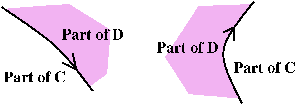 Look back at the rectangle picture. You should see, I hope, that the
boundary is a simple closed curve, which is positively oriented with
respect to the interior. And look again at the semidisc (can't be a
word!). The inside of the semidisc is to the left of the boundary as
the parameter increases.
Look back at the rectangle picture. You should see, I hope, that the
boundary is a simple closed curve, which is positively oriented with
respect to the interior. And look again at the semidisc (can't be a
word!). The inside of the semidisc is to the left of the boundary as
the parameter increases.
- Piecewise smooth
This means that the functions parameterizing the boundary should be
differentiable, or that they should be a finite "sum" of
differentiable functions. For example, a rectangle is a "sum" of four
smooth boundary parameterizations. Here the sum is understood to be in
the sense of curves, where one curve followed by another is sometimes
thought of as adding the curves.
Information transported from the boundary to the inside
Suppose P(x,y)=-(1/2)y and Q(x,y)=(1/2)x. Then
Q(x,y)/x-P(x,y)/y just
"happens" to be 1. And the double integral of 1 over the region is
equal to its area. So apparently C-(1/2)y dx+(1/2)x dy is the area of
D. Let me try to make this even sharper. The curve C should be
parameterized. So x=x(t) and y=y(t) for t between a and b. The line
integral gets translated into the following Riemann integral:
t=at=b-(1/2)y(t)x´(t)+(1/2)x(t)y´(t) dt.
So suppose you are in a race car, driving around a "closed
course". Your position could be measured with a GPS device, so you
would know <x(t),y(t)> (the position vector). You could also
imagine that you have some idea of your velocity:
<x´(t),y´(t)>. So from this "boundary data" you could
compute (at least approximately) the Riemann integral t=at=b-(1/2)y(t)x´(t)+(1/2)x(t)y´(t) dt
and this must be the area of enclosed by the race track. This is
astonishing to me.
People designed interesting mechanical linkages to compute areas based
on such results. These instruments are called planimeters. People can be very clever.
Analogous results in higher dimensions would allow some knowledge of
the heart based upon electrical readings on the skin. Weird,
wonderful, terrific!
Another example, somewhat paradoxical
Here I will tell you what P(x,y) and Q(x,y) should be. These are
certainly not randomly chosen but are specific functions which are
used to model important physical phenomena.
P(x,y)=-y/(x2+y2) and
Q(x,y)=x/(x2+y2)
It just happens (!!) that:
P/y=[-(x2+y2)+y(2y)]/(x2+y2)2=[y2-x2]/(x2+y2)2
and
Q/x=[(x2+y2)-2x(x)]/(x2+y2)2=[y2-x2]/(x2+y2)2.
Therefore in this case, Py=Qx so that
Qx-Py is 0.
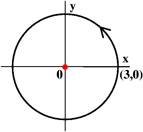 Now let me compute the line integral CP(x,y)dx+Q(x,y)dy, where C is, say, the circle of
radius 3 centered at (0,0). The first parameterization you should
consider is this: x=3cos(t) and y=3sin(t) so that dx=-3sin(t) dt
and dy=3cos(t) dt. Then x2+y2=32
because sin2+cos2=1. Thus
Now let me compute the line integral CP(x,y)dx+Q(x,y)dy, where C is, say, the circle of
radius 3 centered at (0,0). The first parameterization you should
consider is this: x=3cos(t) and y=3sin(t) so that dx=-3sin(t) dt
and dy=3cos(t) dt. Then x2+y2=32
because sin2+cos2=1. Thus
C-y/(x2+y2)dx+x/(x2+y2)dy
becomes t=0t=2Pi([-3sin(t)/32](-3sin(t))+[3cos(t)/32]3cos(t))dt. If the arithmetic is done correctly we need to
integrate 1 from 0 to 2Pi (almost everything cancels!) and the result
is 2Pi.
But but but ... the integrand on the "other side" of Green's Theorem
is Qx-Py and we computed that to be 0. A circle
certainly is a simple closed curve, positively oriented, etc. We
haven't made any errors. Maybe it is true that 2Pi=0? No! That is not true.
Technicalities matter.
I've ignored the requirements on P(x,y) and Q(x,y). Here the
requirements definitely are relevant. Both P(x,y) and Q(x,y), and
their first partial derivatives, are quotients of polynomials, and
have x2+y2 in the denominator (the bottom of the
fraction). That expression is 0 at the origin, (0,0). In fact, P(x,y)
and Q(x,y) and their first partial derivatives are not
continuous at (0,0), which I will call the "bad point". This bad point
is inside the circle. The example shows that even if the hypothesis
"P(x,y) and Q(x,y) are functions with continuous first partial
derivatives" fials at just one point of D, the equality predicted by
Green's Theorem can fail very very emphatically (I think "zero equals
something non-zero" is a fairly emphatic failure).
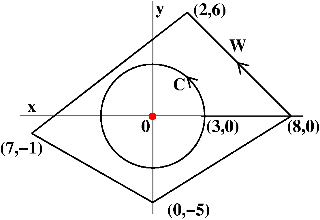
Information transported from one curve to another, using the inside
The example considered is, however, very important in practice. Let me
show why. Let's consider another path, W, which is a quadrilateral. W
is a simple closed curve made of four straight line segments. It
starts at (8,0), goes to (2,6), then to (7,-1), then to (0,-5), and
finally back to (8,0). I would like to compute W-y/(x2+y2)dx+x/(x2+y2)dy. Here
I am not so sure I could "easily" compute the integrals which would
come out of parameterizing the four line segments, and changing the
x,y language to t language. At least the task would be lengthy. So let
me show you another way. Again, I can't just apply Green's Theorem to
W and the region inside W, since W encloses the same bad point. But I
can do something very clever using Green's Theorem.
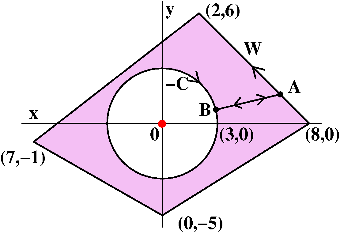
Crosscut
Let me select a point A on W and a point B on C and join them by a
line segment. Now I want to describe a closed curve in the plane, and
this is very very clever. I'll go first from (8,0) on W to A. Then I
will go from A to B on the crosscut. Then around C in reverse (note
that the picture now has the arrowhead on C reversed and the label
states "-C"). Then I go from B to A, and finally, I follow the
remainder of W around to (8,0). What about the integral of
P(x,y)dx+Q(x,y)dy along this path? The integrals on the crosscut line
segments cancel, and the integral on -C is minus the integral along C,
and the remainder is the integral on W. So the result is the integral along W minus the integral along C.
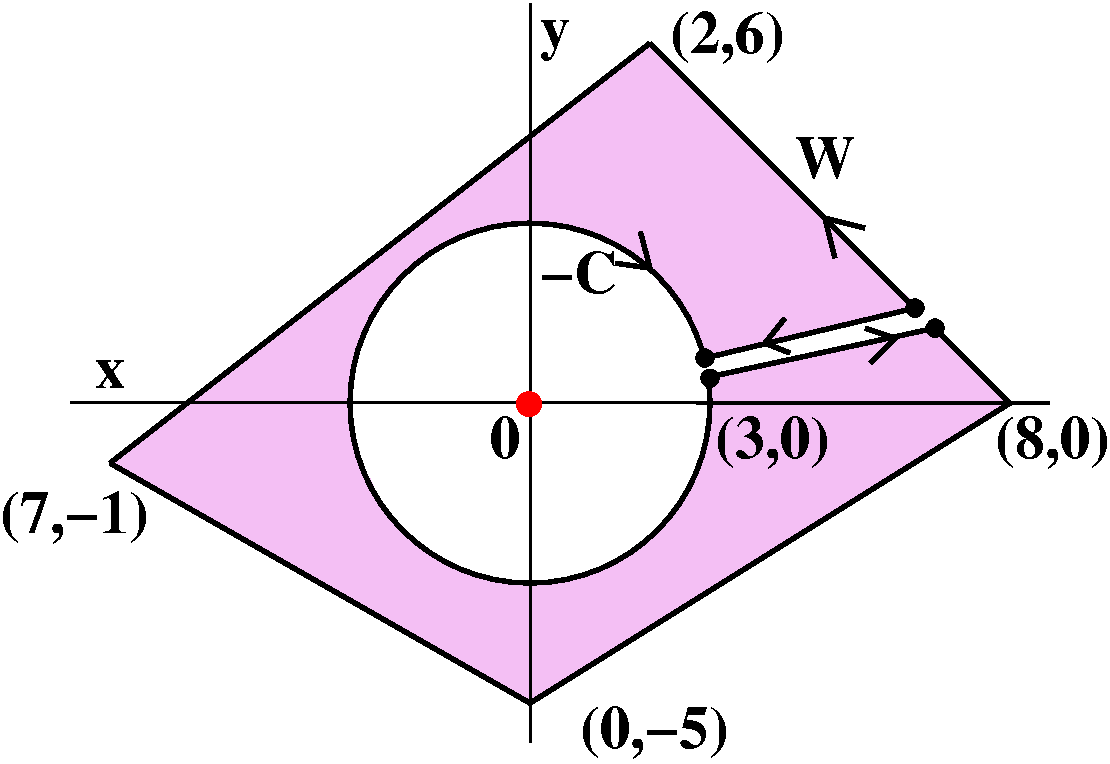
Now let me split up the crosscut into two distinct line segments, one
directed from W to C and one directed backwards. The points A and B
become doubled, and each pair is slightly separated. Now the closed
curve is a simple closed curve. The region this simple closed
curve bounds does not include the origin, the bad point. Inside
the region, Py=Qx and therefore the double
integral side of the Green's Theorem equation is 0. The line integral
side is also 0. This will work for any separation, no matter how
small. Now the line integral will vary quite continuously as the
separation --> 0. And therefore, when the separation=0, the line
integral will still be 0. And so, clearly the integral along W
minus the integral along C is 0 (because the crosscuts cancel!) so the
integral along W is the same as the integral along C: it must be 2Pi!
That clearly may be the worst
clearly in the course. I don't think an accusation of excessive
rigor (too much proving: "the quality of being logically valid") would
be correct in Math 251, and the statement I am asserting as clear
needs proof. What I am asserting is that if one path is close to
another, and if P(x,y) and Q(x,y) are, say, at least continuous, then
the work along the two paths will be close. To me this is physically
reasonable. I hope it is to you.
This crosscutting technique is so familiar to people who use it that
it is rarely discussed in detail. In fact, any curve which goes around
the origin exactly once will have the line integral of our
P(x,y)dx+Q(x,y)dy equal to 2Pi for similar reasons.
A physical model?
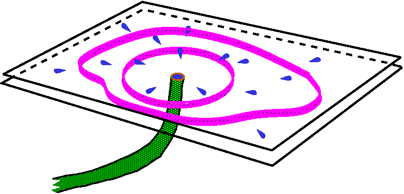 I think the computations I've just done are difficult to understand. I
mentioned the following physical model to some students after
class. Line integrals can also be thought of as measuring flux,
the net flow through the curve. We will investigate this situation in
R3 soon. But consider the following physical setup: two
parallel planes of plastic, and a hose inserted through one of the
planes, pumping water in at a steady rate (the blue things in the
picture are not minnows, they are water drops!). If we surround this
source with some sort of circular detection "fence" then we can
look at how the water goes through the fence, and from that deduce the
rate at which water is being pumped in. But we could also install
another detection fence. If we do the same computations for that
fence, the source rate should be the same, because the hose is pumping
water in steadily: its rate is not varying. The mathematical
computation with the crosscuts above is a version of this physical
situation. When Py-Qx=0, away from the hose (at
the origin) the source rate is 0. Any comprehensive measurement of
flow surrounding the origin will get the same answer.
I think the computations I've just done are difficult to understand. I
mentioned the following physical model to some students after
class. Line integrals can also be thought of as measuring flux,
the net flow through the curve. We will investigate this situation in
R3 soon. But consider the following physical setup: two
parallel planes of plastic, and a hose inserted through one of the
planes, pumping water in at a steady rate (the blue things in the
picture are not minnows, they are water drops!). If we surround this
source with some sort of circular detection "fence" then we can
look at how the water goes through the fence, and from that deduce the
rate at which water is being pumped in. But we could also install
another detection fence. If we do the same computations for that
fence, the source rate should be the same, because the hose is pumping
water in steadily: its rate is not varying. The mathematical
computation with the crosscuts above is a version of this physical
situation. When Py-Qx=0, away from the hose (at
the origin) the source rate is 0. Any comprehensive measurement of
flow surrounding the origin will get the same answer.
Another physical setup which this P and Q model is an isolated point
charge. There the work done in moving around the charge will always be
the same. We will encounter this in three dimensions soon, and maybe
there it will be easier to understand.
Another application (important!) of Green's Theorem
I did not get a chance to discuss this in class. When is a vector
field P(x,y)i+Q(x,y)j conservative? Certainly when it is
a gradient vector field: so there is a potential function, f(x,y),
with f/x=P(x,y) and f/y=Q(x,y). We can try to find f(x,y) by integrating and
matching the descriptions. But this can be difficult and
lengthy. Differentiation is easier, and certainly if
there is a potential, f(x,y), then P/y=Q/x by Clairaut's Theorem. But the example above (the isolated
electric charge or the fluid flow point source) shows that we can have
P/y=Q/x without having a
potential. Why? If we had a potential then the integral around closed
curves would be 0, but we saw that such an integral for out example
may not be 0. If we had no bad points, then the integral around closed
curves would be 0 using Green's Theorem. So any region where
there are no bad points has the converse true:
If P/y=Q/x and there are no
"bad points" for P or Q, then there is a potential.
This can sometimes be very useful because differentiation is
... easier! So people have given a name to regions which have no
holes. So: a region is simply connected if it has no
holes. In such a region, if the condition P/y=Q/x is correct at all points, then
there is a potential, so the vector field is conservative. A disc (the
inside of a circle) is simply connected. But if you remove a point,
the result is not simply connected.
Tuesday, April 4
Restatement and summary of previous results
A vector field is conservative if the work done along paths
depends only on the endpoints of the paths. Such a vector field is
also called path independent. This is logically equivalent to
having the integrals around all closed curves (curves whose
START equals their END) be equal to
0.
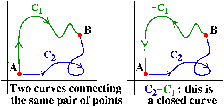 Why?
Why?
Take two points, A and B, in the plane and suppose that C1
and C2 are two paths going from A to B. If the line
integrals along C1 and C2 are equal, then if you
first integrate along C1 and then backwards along
C2 (this is usually called, not surprisingly,
-C2) the net result will be 0. So the integral along any
closed curve will be 0. On the other hand, if you know the integral
around all closed curves is always 0, then you can compare integrals
around two paths, say C1 and C2, from A to B by
just looking at the work done around
C1-C2. Since, by assumption, the integrals
around closed curves are 0, the integral along C1
must exactly be canceled by the integral along
-C2. Therefore the integral along C1 is the same
as the integral along C2: this is path independence.
More restatement and summary
We showed that a gradient vector field is actually path
independent. Even further, if we happen to know a potential,
that is, a function whose gradient is that vector field, then the
integral from START to END will just be the
difference: the value of the potential at the END minus the
value of the potential at the START.
How to answer the previous QotD
So V is
(x3-Ax2y-y3)i+(Bxy2-2x3)j. We're
told that there are values of the constants A and B which make
V a gradient vector field. What are these constants? Here is
one approach, which also "creates" the potential function. The reason
to use this approach is that (looking ahead in the problem) we'll need
to use the potential function to evaluate a line integral. Suppose
f(x,y) is a potential function for V. Then:
f/x=x3-Ax2y-y3
f/x=Bxy2-2x3
Let's integrate the first equation with respect to x (I put
that in bold type because it is easy to get confused about what is
variable and what is constant -- here x is the variable,
and A and y are constants):
f(x,y)=(1/4)x4-(A/3)x3y-xy3+C1(y). The function C1(y) is an antidifferentiation "constant". It could contain any function of y (including just ordinary constants).
The second equation, integrated with respect to y, gives:
f(x,y)=(B/3)xy3-2x3y+C2(x). The
function C2(x) is similar to the previous "constant": it
can contain any function of x.
Now we have two descriptions of the potential, f(x,y):
Description #1
(1/4)x4-(A/3)x3y-xy3+C1(y)
Description #1
(B/3)xy3-2x3y+C2(x)
We can compare and cross-check. Everything should appear exactly once
and only once in f(x,y). So the (1/4)x4 appearing in #1
must be somewhere in #2: ahhh, it is hiding inside
C2(x). The -(A/3)x3y in #1 must be
-2x3y in #2, and therefore -A/3=-2 so that A=6. The
-xy3 in #1 is (B/3)xy3 in #2, and we infer that
-1=B/3 so that B=-3. There's nothing corresponding to C1(y)
in #2, so I might as well (to make my life simpler!) take
C1(y) to be 0. If I were working on an exam (or any time,
actually), I think I would add suspenders to my belt and check the
other way: that is, look at all the terms in #2 and make sure I can
find them in #1. That is indeed true here. I combine all the
information about my description and tell you that a potential for
V is f(x,y)=(1/4)x4-2x3y-xy3.
The second part of the QotD told us that C was a curve starting at
(0,2) and ending at (3,1). We were requested to find the line integral
CV·T ds. We have a potential, so
this is just
f(END)-f(START)=f(3,1)-f(0,2)=(1/4)34-2(33)1-3(13)-0
(all the terms of f(x,y) have an x in them and x=0 at the
START).
Comment If this problem occurred on an exam I gave, I would
want students to leave the answer as it is. Don't touch it -- you
might break it. If you break it, then you "buy" it, and I should
reduce the score.
Another way to find A and B
If we just wanted to find A and B, well, differentiation is almost
always easier than antidifferentiation (that doesn't occur here, with
polynomials). We can use Clairaut's Theorem (equality of mixed partial derivatives) to find A and B. Since
f/x=x3-Ax2y-y3
f/x=Bxy2-2x3
we know that (/y)f/x=(/x)f/y
and therefore (/y)(x3-Ax2y-y3)
must equal (/x)(Bxy2-2x3),
so that
-Ax2-3y2=By2-6x2. Again we
compare these two descriptions of polynomials. If these
descriptions are to be the same, then -A=-6 and -3=B. This leads to
the same values of A and B as we got before. I didn't use this method,
which is frequently quicker than integrating, because I believe the
person who wrote the problem: that there would be values of A and B
making this vector field conservative, and that I would need the
potential to complete the problem. If I just done the differentiations
here, then I still would have had to integrate to get a potential.
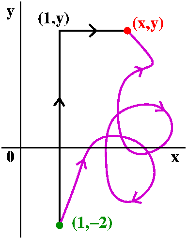 Another way to find a potential
Sometimes in physics and engineering applications there are reasons to
"prefer" one point in the plane to another. This sounds awfully silly,
but ... it does occur. When this happens, "construction" of a
potential can be done by paying attention to this specified
point. I'll call the specified point, "the ground state". Here in this
example I'll use (1,-2) as the ground state. This is certainly
artificial, but the choice will illustrate the method.
If someone gives me a vector field which is guaranteed path
independent, then I might want to believe the potential could be
revealed by making measurements relative to the ground state. I might
take paths from (1,-2) to (x,y) and call the work done f(x,y). Since
the vector field is supposed to be path independent, the choice of
path won't matter. I don't think I would take the silly curvy path shown. That's hard
to work with. Indeed, as I mentioned in class, almost all of the paths
you're likely to see in "real life" will be line segments and arcs of
circles. I'd probably take the path shown, a line segment from (1,-2)
to (1,y) and then a line segment from (1,y) to (x,y). An alternative
suggested by students is the direct trip: from (1,-2) to (x,y) and
that is certainly used some of the time, but I am lazy (I don't want
to compute the darn tilted line!).
I will write this as a sum of two integrals:
f(x,y)=Vertical segment(x3-6x2y-y3)dx+(-3xy2-2x3)dy
+ Horizontal segment(x3-6x2y-y3)dx+(-3xy2-2x3)dy
What's going on?
Why shouldn't the integral over closed curves always be equal to 0?
A computation
A realization
Example
Green
Diary entry in progress! More to
come.
Friday, March 31
Diary entry in progress! More to
come.
Irrelevant (?) computations while preparing for the exam
I did several chain rule computations. The first was something like
what follows but easier (only polynomials inside):
if z=f(5cos(x)+3ey) and f is a differentiable function of
one variable, compute some partial derivatives of z with respect to x
and y.
z/x
Use the chain rule. The result is f´(5cos(x)+3ey)(-5sin(x)).
z/y
Use the chain rule. The
result is f´(5cos(x)+3ey)(3ey).
2z/x2
Use the chain rule and the product rule beginning with the very first
result about z: differentiate zx with respect to x.
So we get
f´´(5cos(x)+3ey)(-5sin(x))2+f'(5cos(x)+3ey)(-5cos(x)).
A more difficult example might be f(7cos(x)e2y).
A second example
I think I then did an almost useful two variable example. Suppose that
z=f(x,y), where f is a differentiable function of two variables, and
x=r cos() and
y=r sin().
z/r
This is (f/x)·(x/r)+(f/y)·(y/r)= (f/x)cos()+(f/y)sin()
z/
A line integral
Let's look at the curve
x(t)=-cos(t)
y(t)=sin(t)+4cos(t)
for t in the interval [-Pi/2,Pi]. This is the curve C.
Let's look at the "force field" (vector field)
F=3i-xj.
To the right is a picture of the curve. It goes from the
START at (0,1) (plug in t=-Pi/2 in the equations for x(t) and
y(t)) to END at (-1,4). It seems to be and is three-quarters
of a tilted ellipse.
The work integral CF·T ds which I immediately
translate to C3 dx-x dy. Since we are given a
parameterized C, I retranslate to t-land:
x(t)=-cos(t) leads to dx=sin(t)dt
y(t)=sin(t)+4cos(t) leads to dy=[cos(t)-4sin(t)]dt
The dictionary gets us
t=-Pi/2 [START]t=Pi [END](-3cos(t)-{-cos(t)}[cos(t)-4sin(t)])dt
and we can multiply etc.:
t=-Pi/2t=Pi(-3cos(t)+cos(t)2-4cos(t)sin(t))dt
Another line integral
 The path I wanted here was a line segment from (0,1) to (-1,4). This
path is shown to the right. In vector notation, we want
(1-t)<0,1>+t<-1,4>. This takes us from t=0 at (0,1) to
(-1,4) at t=1.
The path I wanted here was a line segment from (0,1) to (-1,4). This
path is shown to the right. In vector notation, we want
(1-t)<0,1>+t<-1,4>. This takes us from t=0 at (0,1) to
(-1,4) at t=1.
Understanding what we did
We showed that work done by the same vector field between the same
pair of points can depend on the path traveled. This is actually
realistic. If you push a marble from point A to point B, then the
local conditions of the path (friction, slipperiness, etc.) can matter
a great deal.
Computationally what we did was really fairly
straightforward. We took the work, turned it into a
P dx+Q dy integral, then parameterized and turned everything
into t-land. And we computed.
Conceptually I would like to try to understand why there is a
difference in the work done. I would like to understand when the work
is the same.
Abstract version of the computation
What if ...
the vector field involved was a gradient vector field?
Consequences, prose version
A conservative vector field is one where the work done along
paths depends only on the start and end points. Such a vector field is
also called path independent. This condition is the same as
asking that the integrals along closed curves (where the
starting point and ending points agree) must always be zero.
If a vector field is a gradient vector field so that it is the
gradient of a function called a potential of that vector field,
then that vector field is conservative. The work done along a
curve is equal to the value of the potential at the end of the curve
minus the value of the potential at the start of the curve.
Gravitation
For example, the inverse square law we introduced is conservative
because it is a gradient vector field. We can verify this by
exhibiting a potential, and the validity of being a potential can be
checked with two derivative computations. Then all work integrals will
be "easy".
Vocabulary
Conservative
Closed curves
Gradient
Potential
The earlier example
is not a gradient vector field.
Reason #1: it is not conservative
Reason #2: try to create a potential
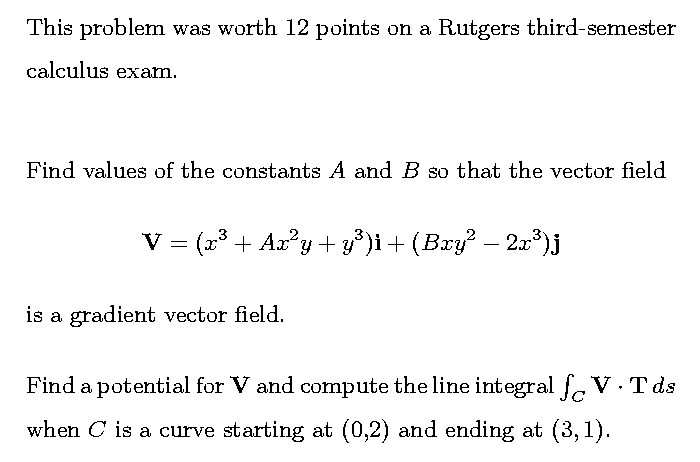 An exam question as the QotD
Diary entry in progress! More to
come.
HOMEWORK
Prepare the
Maple assignment. Read and do the syllabus problems for
16.3. Look at the review questions and select one or two at random and
write out solutions. If I don't have the solutions posted already,
then send them to me, please. I will check them and post them, thank
you then.
Tuesday, March 24
 This morning I observed a Song Sparrow, Melospiza melodia,
pictured to the right, at my bird feeder. As I entered SEC at 8:40 AM
(almost on time!) I heard and saw a Chipping Sparrow, Spizella
passerina, pictured to the left. The significance of both events
is that these birds are summer residents of central New Jersey. Spring
definitely is here! Hooray!! By the way, I do not offhand know
the Latin (Linnean) names of the bird species. I look them up, and put
them here because I want to be a good academic.
This morning I observed a Song Sparrow, Melospiza melodia,
pictured to the right, at my bird feeder. As I entered SEC at 8:40 AM
(almost on time!) I heard and saw a Chipping Sparrow, Spizella
passerina, pictured to the left. The significance of both events
is that these birds are summer residents of central New Jersey. Spring
definitely is here! Hooray!! By the way, I do not offhand know
the Latin (Linnean) names of the bird species. I look them up, and put
them here because I want to be a good academic.
Maple
If you did not get information about the third Maple
assignment, please send me
e-mail immediately. Messages were sent out by midday
Saturday. This assignment is somewhat longer than the previous two
assignments and likely will need more time.
Exam
There will be an exam on Friday, April 7. A draft formula sheet has been
prepared. Please look at it. I don't want any further mistakes to
occur, and you could also advise me if you think something important
is not there. Some review problems
have also been prepared. I hope that students will write solutions to
some of these problems. These solutions can be sent to me. I will
proofread them, and post them. Everyone can benefit from this. There
are a number of review problems, and they probably can't all be done
the night before the exam! The sheet of review problems also contains
information about what will be tested by the exam.
Irrelevance awards
I asked in the last diary entry for the identity of the individual
pierced by arrows and for the painter. The answers are, respectively,
St. Sebastian and Andreas Mantegna
(c. 1431-1506). St. Sebastian was martyred c.288 at Rome. I found the
following information which I did not know before:
|
During the 14th century, the random nature of infection with the Black
Death caused people to liken the plague to their villages being shot
by an army of nature's archers. In desparation they prayed for the
intercession of a saint associated with archers, and Saint Sebastian
became associated with the plague.
|
Four students responded from the class responded with identifications,
and these four students have received professionally selected and
packaged awards. Their names are
Demetrio Koloseus-Ganon and Ralitza Varlakova and
Christopher Martin and Chirag Walawalkar.
I thank them
for their effort and interest.
Look at these names. Isn't Rutgers wonderfully
diverse?
Vector fields
- Geometrically, a vector field "is" a collection of arrows in the
plane.
- Algebraically, a vector field "is" a pair of functions,
f(x,y)i+g(x,y)j.
The simplest ways students discover vector fields in their studies
is:
Force fields A typical example is the inverse square
"law" analyzed last time.
Fluid flow A vortex is one example. Explicitly, it was
-yi+xj. This sort of describes a swirling flow around
the origin.
Gradient vector fields We haven't discussed this so far, and
these are an important type of vector fields.
Gradient vector fields
This could be in either two or three variables. Let's suppose for
simplicity we have a function F(x,y) of two variables. Then the
gradient of F is F=[F/x]i+[F/y]j is a vector field: it is
a function multiplied by i plus a function multiplied by
j.
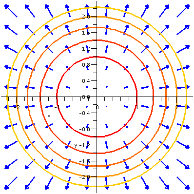 An example
I looked at F(x,y)=x2+y2. Here I recalled that
the contour lines were x2+y2=Constant. These are
all circles centered at the origin. If we draw a collection of contour
lines for equally spaced constants (for example, for 1 and 2 and 3 and
4 and ...) then it turns out that the lines get closer and closer
together as the equally spaced constants increase. This is because the
function is increasing more rapidly as x and y get larger in absolute
value. The associated gradient vector field is
2xi+2yj. At (x,y), these vectors are perpendicular to
the circles and point away from the origin in the direction of
increase of F. As (x,y) "moves" farther from (0,0), the magnitude of
the vectors increases.
To the right is a picture of this gradient vector field together with
some contour lines. Previously I had defined F:=x^2+y^2;. The
picture displays the output of these Maple
commands:
> contourplot(F,x=-2.5..2.5,y=-2.5..2.5, thickness=2,
contours=[1,2,3,4,5], grid=[40,40]);
>
fieldplot(2*x,2*y],x=-2.15..2.15,y=-2.15..2.15,arrows=slim,grid=[10,10],
fieldstrength=maximal(.9)color=blue,thickness=2);
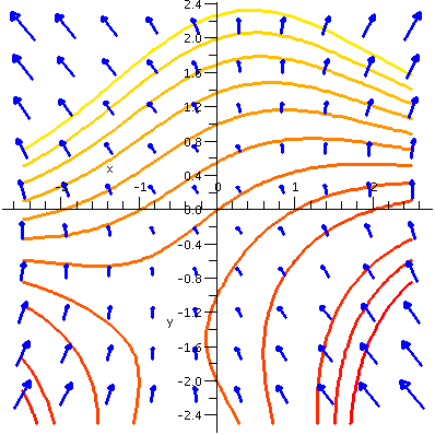 Another example
This example uses a function which is less symmetric and less
simple. The function is x2y-2x+y2+3y. The level
curves are shown for the values -12, -10, -8, -6, -4, -2, 0, 2, 4, 6,
8, and 10: the even integers from -12 to 12. Notice that the arrows
seem to be perpendicular to the level curves, and that the arrows are
longer when the spacing between the contour lines (corresponding to
equal differences in the constants) gets closer.
Comment
I looked at this picture and wondered what the
heck happened where the arrows got really small. What does
happen? Well, we can look for a critical point: Fx=2xy-2=0
and Fy=x2+3y+3=0. The first equation
tells me that y=1/x and then the second equation becomes
x3+3x+3=0, and I can't "solve" that. So I asked
fsolve and was told there was one critical point, at
(approximately) x=-.596 and y=1.678: this looks correct. What kind of
critical point? (Max/min/saddle) If you look at the picture and the
level curves you can probably guess. I actually computed the Hessian,
and it is a saddle. Ain't math fun?
In general ...
What was written above is generally true about a gradient vector field
and the contour lines or curves (contour surfaces in
R3). That is, the gradient vector field "arrows" are
perpendicular to the level curves. They "point" towards increasing
values of the function. Their magnitude (the length of the arrows) is
a measure of the density (?) of the contour lines: if the function is
rapidly changing then the length will be longer.
By the way, if F=V,
then F is called a potential of the vector field,
V. The word and concepts connected with it are important in
physics. I'll discuss more about this during the next class.
Is the vortex flow a gradient vector field?
Look at -yi+xj. Is this vector field a gradient vector
field? If it is, can we find a potential for it? If it is not, can we
explain why? This turns out to be a serious and interesting question,
because of things we will learn very soon (Friday). Also it has some
interesting physical consequences. Well, here is one way to decide the
answer.
Suppose F(x,y) is a potential for -yi+xj. That
means
      /y
Fx=-y -----> Fxy=-1
      /x
Fy=x  -----> Fyx=1
But "mixed" partial derivatives are supposed to be equal (that is, if
some hypotheses are satisfied, but these are all very reasonable
functions and nothing weird happens). Since -1 is not equal to 1 (this
week?) we know that the vortex flow is not a gradient vector
field. I don't think this is an obvious fact.
Line integrals
We need an additional technical tool to investigate vector fields:
line integrals. Line integrals will allow the computation of work for
force fields, and flux for fluid flow, and something for gradient
vector fields. Work and flux and other things are important physical
quantities and turn out to have nice mathematical properties. So here
we go.
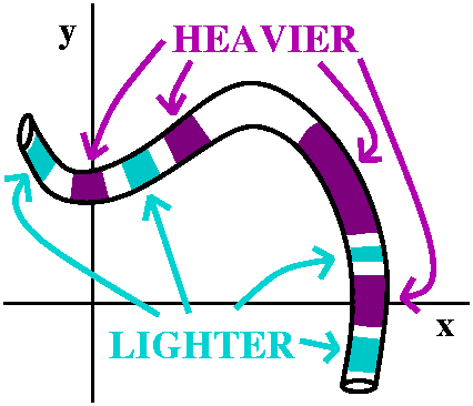 Mass of a wire
I'll introduce line integrals using the metaphor of the mass of a wire.
The integral calculus mantra is:
chop up, approximate, sum, limit.
Here I'll assume that there is a wire sitting in R2. Its
geometry is simple, with a constant cross-sectional area (assumed to
be 1 in the measurement system used). The density of the wire will
vary according to the position on the wire: at some points the density
will be high, and the wire heavy, and at other points, the density
will be low, and the wire rather light. The task is to create some
technical tool which will represent the total mass of the wire. By the
way, the accompanying picture looks like a particularly ugly
worm or snake. I am sorry.
Suppose I cut the wire up into lots of little chunks. How little?
Well, the length of each chunk will be ds, a tiny piece of arc length
(we discussed this in several lectures given late January, long, long
ago). If I assume that the density D(x,y) varies only a small amount
because the chunk of the wire is very small, then dm, the mass of this
piece, is nearly D(x,y) ds (remember I made the cross-sectional
area equal to 1). Further, I can add up these pieces of mass to get
the total mass. I can take the limit as the number of pieces gets
large and the length of the pieces gets small. The result is that the mass
of the wire should be given by
The wireD(x,y) ds.
This integral is called a line integral, where the word
line doesn't mean "straight line" but is used in the sense "A
thin continuous mark, as that made by a pen, pencil, or brush applied
to a surface." Now I need to show you what this means. So I will
compute a very artificial example.
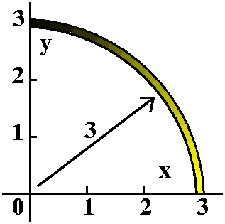 Silly example
My example was the following: the wire follows the part of the circle
of radius 3 which is in the first quadrant. The density of the wire at
the point (x,y) is 7y+5. Find the mass of the wire. Well, I will take
the integral The wireD(x,y) ds and parameterize
everything in sight. To me the natural parameterization of an arc of a
circle uses essentially the angle from the center. The text likes to
use t here, so I will parameterize this quarter circle with x=3cos(t)
and y=3cos(t). The interval of this parameterization is [0,Pi/2]. Now
ds is sqrt([dx/dt]2+[dy/dt]2) dt. The
square root stuff is the magnitude of the velocity vector, the
speed. And ds=SPEED·dt is a translation of
distance=rate·time of course. In this case, dx/dt=-3sin(t) and
dy/dt=3cos(t) so that
sqrt([dx/dt]2+[dy/dt]2) just happens (!!!) to
simplify to 3. And ds=3 dt. What about the density? Since
D(x,y)=-7y+5, we know that the density is 7(3sin(t))+5. And the
integral should go from 0 to Pi/2. Therefore
The mass=The wireD(x,y) ds=t=0t=Pi/2{21sin(t)+5}3 dt=-63cos(t)+15t]t=0t=Pi/2=63+(15/2)Pi.
This is a totally insignificant, physically unrealistic (to me)
computation. The only thing I had fun with is drawing the picture,
which with its varying colors is supposed to suggest the increasing
density of the wire as y increases. There is one very important
fact which should be mentioned now:
Independence of parameterization
In this line integral and in all line integrals, the result will be
the same no matter which parameterization is used. Verification of
this uses the one variable chain rule and is not too interesting right
now. So let me go on.
Random example
I then featured a really random example. I asked students for some
random (positive) integers which I then used to construct an example
very much like the one presented in what follows. The previous example
was arranged so that ds was nice. I now tried to compute something
like the mass of a wire where the wire was sitting on the curve
y=x4 from, say, (0,0) to (2, 16), and the density is
D(x,y)=x4y7. I not being totally idiotic
here. Any computational strategy in calculus should be able to handle
low-degree polynomials fairly efficiently, even by hand. So here's
what we did.
A simple parameterization of a graph of a function is just to use the
independent variable as the parameter. So I used x=t and
y=t4 and then the density x4y7 became
t4(t4)7=t28. This isn't
too bad, but I am saving the worst for last, and in this computation
the worst is ds. So dx/dt=1 and dy/dt=4t3,
and therefore ds/dt=sqrt(1+16t6). The line integral for
this "mass" translates in t-land as follows:
The wireD(x,y) ds=t=0t=2t28sqrt(1+16t6)dt.
This integral cannot be computed exactly in terms of standard
"familiar" functions. I found to my amazement that Maple does
have a storehouse of weird functions which it can use to "evaluate"
this integral. But then I have no feeling for the functions it used
and certainly not for the values of the functions.
ds is the obstacle
What is horrible about most line integrals is ds. Almost no ds except
for those included in textbook problems lead to familiar
antiderivatives. At the same time, important quantities such as work
and flux are defined as mathematical objects in terms of line
integrals, and the general expectation is that these quantities
can be computed exactly in terms of familiar functions.
To me this is an excellent example of the psychological phenomenon
known as cognitive
dissonance:
| Cognitive dissonance arises from conflicting
cognitions. Cognitive dissonance is the perception of incompatibility
between two cognitions, which for the purpose of cognitive dissonance
theory can be defined as any element of knowledge, attitude, emotion,
belief or value, as well as a goal, plan, or an interest. In brief,
the theory of cognitive dissonance holds that contradicting cognitions
serve as a driving force that compels the mind to acquire or invent
new thoughts or beliefs, or to modify existing beliefs, so as to
minimize the amount of dissonance (conflict) between cognitions.
|
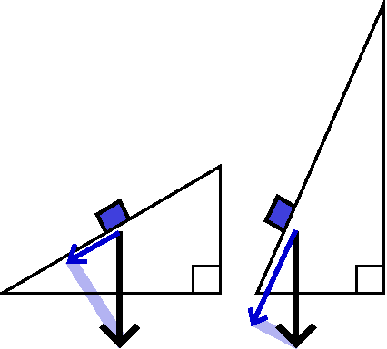 Work
Work
Let's consider the physical concept called work. This is
"force" times "distance", loosely, but we're going to need to be a bit
more specific. For example, consider a mass being pushed up a
frictionless triangle. If the triangle is steeper, then more force is
needed. In the picture, the force of gravity is directed down. The
blue arrows on each inclined plane (triangle) show the force component
needed to move the box up that triangle.
So instead of dieting, avoid steep triangles and your weight
will decrease ... no no no
... this is just more bad information from the lecturer!
Anyway, what really matters is the component of the force in the
direction of motion (we could take the dot product of the force and
the displacement also).
Work with a varying vector field along a curve
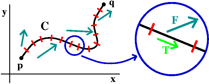 Again, chop up, approximate, sum,
limit.
Again, chop up, approximate, sum,
limit.
I would like to describe how to compute the work done against a
varying force field F as we travel from p to q (in
R2 but the same ideas will work in R3, also)
along a curve, C. We chop up C into small pieces (the red lines are
the chopping places). One of them is displayed under a "magnifying
glass" (sort of) in the picture. The piece is so small that it is
almost a straight line, and its length is ds. The piece is also so
small that the vector field, F, is almost constant near the
piece. Remember that a unit tangent vector, pointing in the direction
of the piece, is called T (go back and think of January!). Then
the part of the force field along the curve is F·T and
the piece of the work will be approximately F·Tds. All
of the work will be the integral along C of this quantity. Therefore
the work is CF·Tds.
A computation
Let us "test" this definition with a random computation: well,
sort of "random". C will be the curve y=x4 and p will be
the point (0,0) and q will be the point (2,16). I will have the force
field be
x2y3i+xy5j. Now let
us compute. We need to change everything
into t-land, where I will choose a most routine parameter: x=t so that
y=t4.
ds
As before, the speed becomes
sqrt([dx/dt]2+[dy/dt]2)=sqrt([1]2+[4t3]2)=sqrt(1+16t6)
which is horrible enough. Thus ds=sqrt(1+16t6)dt.
F
At the point (x,y), F is
x2y3i+xy5j so that at
(t,t4) on the curve, F is
t2(t4)3i+t(t4)5j=t14i+t21j.
T
Now comes almost the miracle. In the movie Shakespeare in Love,
one character states, "The natural condition is one of insurmountable
obstacles on the road to imminent disaster." He then says almost
immediately, "Strangely enough , it all turns out well." When asked
"How", the character replies, "I don't know. It's a mystery." So, if
not a miracle, let me show you the little mystery here.
The unit
tangent vector, T, is a vector in the direction of the
curve. The position vector of the curve is <t,t4> so
that the velocity vector is <1,4t3>. But we need a
unit vector to get the projection of F in the direction
of the curve. Divide by the magnitude of
<1,4t3>. Therefore,
T=<1,4t3>/sqrt(1+16t6).
Assembling the work integral
CF·Tds=t=0t=2(t14i+t21j)·
(<1,4t3>/sqrt(1+16t6))sqrt(1+16t6)dt. This is
t=0t=2t14+4t24 dt.
which with totally routine polynomial calculations can be evaluated:
it is 215/15+(4/25)225.
What happens?
The speed comes in to squeeze down the velocity vector to get the unit
tangent vector. The speed comes in as the factor which multiplies dt
to get ds. The two appearances of the speed cancel. They will always cancel!.
Using the notation to help
Here is how people use notation to guide their way through the
computation. No one computes the speed (the square root stuff) when
computing work because it will cancel. So:
Problem statement
Compute the work if
F(x,y)=x2y3i+xy5j
and the curve is y=x4 going from (0,0) to (2,16).
A solution
So I initially write CF·Tds but then I immediately change
to Cx2y3dx+xy5dy. I
evaluate this line integral again by changing everything to t-land. So
x=t and y=t4 and dx=1dt and dy=4t3dt, Also,
x2y3=t2(t4)3=t14
and
xy5=t(t4)5=t21. Therefore
x2y3dx+xy5dy=t14dt+t214t3dt.
Therefore Cx2y3dx+xy5dy=
t=0 [START]t=2 [END]
t14+4t24dt. And the result will be the
same. Almost everyone uses this notation, and never bothers with
computing T and ds and then canceling, etc. Of course, the
ideas are important: the physical quantity we are computing has
certain properties (wait until Friday!) which make this computation
extremely interesting.
QotD
What is the work done if F is the vector field
x2i+yj is and the curve is x=t and
y=t3-t as the parameter goes from t=0 to t=1? The answer
turns out to be 1/3.
Caution!!!
I just read students' answers to the QotD. Many people did this
problem completely correctly. Many others clearly had the ideas
correct but made one or two or three algebra or
arithmetic errors. This sort of thing can really hurt you on
exams!
The word iatrogenic refers to illnesses or other problems
"caused by medical examination or treatment." Please don't let your
solutions make the problems worse!
HOMEWORK
Keep reading
chapter 16. I will discuss conservative vector fields, etc. (16.3) on
Friday. Please be there.
Friday, March 24
Exam?
There may be an exam two weeks from today. More definite information
will be available next week.
Maple?
I hope that either today or tomorrow information about the third
Maple lab will be sent to students. This lab will be worth
20 points (!). Please watch for e-mail.
Spherical coordinates
I drew the same picture I showed last
time. I deduced the following formulas (with errors but they were
corrected):
x=(rho)sin(phi)cos()
y=(rho)sin(phi)cos()
z=(rho)cos(phi)
I remarked that it was useful to know that such formulas existed, but
that I had rarely used them. One result that I have used frequently
comes from the fact that rho represents the distance from (x,y,z) to
the origin.
x2+y2+z2=rho2.
Standard restrictions on spherical coordinates
Because the angles sort of fold over when Pi's and 2Pi's are added,
most people who use spherical coordinates put some restrictions on how
big/small and phi can be. If we only allow to be between 0
and 2Pi and only allow phi to be between 0 and Pi, then there will be
unique spherical coordinates for every point in R3. So I
will generally work with these restrictions.
Some shapes in spherical coordinates
|
rho=constant gives a sphere centered at the origin. So, for example,
rho=5 is a sphere centered at the origin of radius 5.
|
phi=constant gives a right circular cone whose axis of symmetry is the
z-axis. For example, phi=Pi/6 is a cone with vertex at the origin and
whose axis of symmetry is the positive z-axis. The angle between the
positive z-axis and any of the cone's "generators" (lines from the
vertex on the surface of the cone) iw Pi/6 (yes, 30o). The
bottom half of the cone is not included because that is where phi is
between Pi/2 and Pi.
|
=constant gives a half-plane, with the z-axis being the edge of
the half-plane. For example, =Pi/4 gives a half-plane which is
perpendicular to the half-line y=x (x>0) in the xy-plane. The other
half of the plane is where is 3Pi/2, and so it is not included
in this obhect.
|
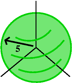 |
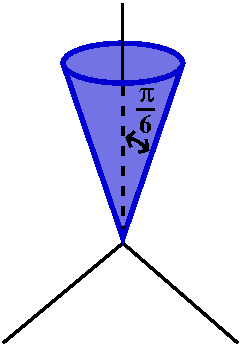 |
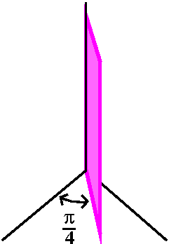 |
Integral #1
A spherical region of radius R is filled with material whose density
is directly proportional to the distance from the origin. What is its
mass?
This is not very realistic. The center is light and
fluffy and the outer edge is heavy and tough (my kind of
cooking?). The density is supposed to interpolate linearly between
these extremes. Maybe the appropriate assignment would be to build an
object of this type.
The math setup
Take a small piece of volume, dV, in the sphere. The corresponding
piece of mass, dm, is related to dV by dm=(density)dV. We know that
the "density is directly proportional to the distance from the
origin." Place the origin of the coordinate system at the center of
the sphere. So there is some constant C>0 so
density=C rho. And the total mass is the sum of the dm's. This
"sum" should be a triple integral:
Total mass=The whole ballC rho dV.
In spherical coordinates, a description of a sphere of radius R
centered at the origin is easy: rho goes from 0 to R, goes from
0 to 2Pi, and phi goes from 0 to Pi. We just use the agreed upon
ranges for the angles to sweep out a whole sphere. There is one sticky
point, however.
dV in spherical coordinates
We need to convert dV to spherical coordinates. In fact,
dV=(rho)2sin(phi)d(rho)dd(phi)
I know this is true. First, there is a diagram which is supposed to be
convincing in the text (figure 8, page 1035). Second, I said it in
class. Third, I actually can give an understandable argument if there
is enough time later in the course. In any case, when I use spherical
coordinates, I almost never bother thinking about this weird mess, but
I just write it.
Vocabulary Several students commented that the "weird mess" is called
the Jacobian, which is how area or volume is distorted with a change
of coordinates. Again, if there is time I'll discuss Jacobians later
in the course (see 15.9 for more information right now, if you'd
like).
The computation
So we have
Total mass=phi=0phi=Pi=0=2Pirho=0rho=R(C rho)(rho)2sin(phi)d(rho)dd(phi).
The inner integral
rho=0rho=R(C rho)(rho)2sin(phi)d(rho)=rho=0rho=RC(rho)3sin(phi)d(rho)=Csin(phi)(rho)4/4]rho=0rho=R=Csin(phi)R4/4.
The middle integral
=0=2PiCsin(phi)R4/4 d=(2Pi C)sin(phi)R4/4=[(Pi C)/2]sin(phi)R4.
(Just multiply by 2Pi, since there is no in the integrand.)
The outer integral
phi=0phi=Pi[(Pi C)/2]sin(phi)R4d(phi)=-[(Pi C)/2]cos(phi)R4]phi=0phi=Pi=(Pi C)R4.
I don't know any way to check this answer. Build a model? Weigh it?
Is this silly?
Well, yes, it is silly. The problem is invented and certainly designed
exactly for spherical coordinates. But I would not use spherical
coordinates, which definitely have peculiarities (look at the pictures
above and look at the expression for dV) unless both the region and the integrand
can both be described in a nice fashion with spherical coordinates. I
won't use this coordinate system otherwise. (Could you imagine using
spherical coordinates to describe a cube?)
Integral #2
Consider the region in the first octant consisting of points whose
distance to the origin is at least 1. Imagine that this is filled with
material whose density is inversely proportional to the fifth power of
the distance to the origin. What is the mass of this object?
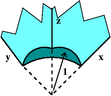
Translating
All of R3 is divided into eight parts by the coordinate
planes: x=0, y=0, and z=0. Each part is called an octant. While
the corresponding regions in the plane (the quadrants) have individual
designations, the
only octant that is named is the first: the octant where
x>0 and y>0 and z>0. In this first octant, I'm
excluding points whose distance to the origin is less than
1. What does the remaining region look like? I think the best picture
I drew in class was one looking at the octant from the back, so here
is a version of that picture. In this picture (sort of the corner of a
rectangular box), a spherical "bite" has been taken out of the
corner. The bite is centered at the vertex (the origin) and has radius
1. Wow!
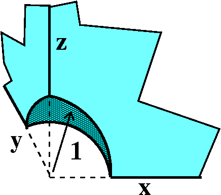 To the right is a more oblique view of the octant with the bite.
The nice thing about this region is that it can be described very briefly
in terms of spherical coordinates. Certainly, rho will go from
1 (as close to the origin as the bite will let us get) out to ... out
to ... infinity (an improper integral!). What about and
phi? Here students should look closely at the definitions of and
phi. Each of them will go from 0 to Pi/2. This is best confirmed by
taking "angles" with vertex at the origin and a side along the x-
(respectively, z-axis) and then opening the second side of the angle
to an aperture of Pi/2 (I think "aperture" means the angle's opening).
To the right is a more oblique view of the octant with the bite.
The nice thing about this region is that it can be described very briefly
in terms of spherical coordinates. Certainly, rho will go from
1 (as close to the origin as the bite will let us get) out to ... out
to ... infinity (an improper integral!). What about and
phi? Here students should look closely at the definitions of and
phi. Each of them will go from 0 to Pi/2. This is best confirmed by
taking "angles" with vertex at the origin and a side along the x-
(respectively, z-axis) and then opening the second side of the angle
to an aperture of Pi/2 (I think "aperture" means the angle's opening).
By the way, as I remarked in class, this is actually a more realistic
example than the first integral. Things like this do occur in
electricity and magnetism.
The computation
Again dm=(density)dV=[C/(rho)5]dV because "density is
inversely proportional to the fifth power of the distance to the
origin." And we know the limits from the discussion above, so the
total mass is
phi=1phi=Pi/2=0=Pi/2rho=1rho=infinity[C/(rho)5](rho)2sin(phi)d(rho)dd(phi).
The integrand is [C/(rho)3]sin(phi) after cancelling some powers.
The inner integral
This is an improper integral, so I will be careful.
rho=1rho=BIGC/(rho)3sin(phi)d(rho)=-C/(2(rho)2)sin(phi)]rho=1rho=BIG=-C/(2(BIG)2)sin(phi)
+C/(2(1)2)sin(phi). As BIG-->infinity, the
term -C/(2(BIG)2)sin(phi)-->0 so the improper
integral
rho=1rho=infinityC/(rho)3sin(phi)d(rho) converges and its value is
(C/2)sin(phi).
The middle integral
=0=Pi/2(C/2)sin(phi)d=(C/2)sin(phi)(Pi/2)=[(C Pi)/4]sin(phi).
The outer integral
phi=0phi=Pi/2[(C Pi)/4]sin(phi)d(phi)=-[(C Pi)/4]cos(phi)]phi=0phi=Pi/2=[(C Pi)/4]
Again, I will admit that I don't know any way to check this
answer. When such an integral comes from a real physical problem,
there is frequently some way to see if the final answer is reasonable.
Further defense of silly (the same defense)
I would only use this technique, I hope!, where both the region
and the integrand are suitable. So, although the problems may have
seemed silly, they are the sort of applications which might occur. We
will need integration in spherical coordinates a few times later in
the course.
Where are we? Where are we going?
About 75% of the course has gone by. Much of what we've done will be
very useful for many of the students, but, perhaps, some of what
we've done will be neeeded less often (I am trying to be
"diplomatic"). The last portion of the course, about what is
frequently called Vector Calculus, can help students understand
many complicated "things" they will likely encounter.
For example, consider a big "chunk" of "stuff". Look at the heat in
the chunk. Sometimes some of the heat might originate inside the
object, and sometimes there might be cooling. And there are also
boundary effects. If there's something really hot near part of the
boundary, heat will flow in around that part, and, similarly, there
might be cool things (?) near some other part of the boundary, and
heat will flow out that part of the boundary. This is all very
complicated. Somehow, there should be some way of balancing the heat
sources and sinks inside the region, and the boundary flow of heat,
and expressing this in some neat way. We'll try to understand this.
The Fundamental Theorem of Calculus, one of the wonderful results of
calc 1, is something like this:
If F´=f, then x=ax=bf(x) dx=F(b)-F(a)
This is a wonderful result. Think about it. It states that some sort
of stuff inside the interval [a,b] (we could think about height times
width, f(x)dx, or some accumulation of "stuff": f(x) inside [a,b] and
added up over the whole interval, [a,b]) is equal to an edge
quantity. There isn't much "edge" to an interval. Here the edge
quantity is F(b)-F(a). You can, with some effort, see things as some
sort of balance between interior accumulation and stuff in and out
the edges. The remainder of the course is an effort to generalize this
to dimensions 2 (Green's Theorem) and 3 (Divergence Theorem) and
dimension (sort of) 2.5: Stokes' Theorem and Gauss's Theorem. These
results provide a language for considering edge effects compared to
inside effects for things like heat flow and fluid flow and ... lots
of other phenomena. So please listen and look carefully. We still
need to learn a few more vocabulary notions.
Vector fields
I'm going to begin with two dimensional vector fields, since the
pictures are easier to draw. Those of you who have seen Euler's method
in calculus will remember bunches of arrows in the plane. So in the
most elementary sense, a vector field is such a "bunch of arrows". In
fact, it is an arrow, a vector, sitting at every point, (x,y).
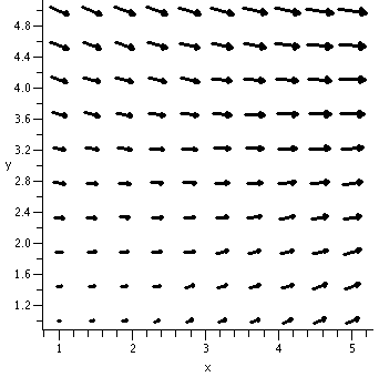 To the right is a "picture" of part of a vector field. The picture was
produced by Maple using a command I learned only
recently (there are thousands of commands, and I believe I know less
than a tenth of one percent of them). This command is in the
plots package. The picture was produced by
To the right is a "picture" of part of a vector field. The picture was
produced by Maple using a command I learned only
recently (there are thousands of commands, and I believe I know less
than a tenth of one percent of them). This command is in the
plots package. The picture was produced by
fieldplot([x^2+10*y,3*x-y^2], x=1..5,y=1..5, arrows=slim,
grid=[10,10], fieldstrength=maximal(.9), thickness=2);
This vector field is the vector
(x2+10y)i+(3x-y2)j at the point (x,y). The
Maple command sketches a few of the arrows ([10,10] gives 100
of them). Sometimes such a picture of a vector field can be very
helpful.
Models?
Vector fields are mathematical models of some basic physical
phenomena. Two that are immediate are force fields and fluid flows.
The force field (gravity, electromagnetism, etc.) might be the
simplest. The "arrow" at every point denotes the presence of a "force"
which can act on the proper kind of object (gravitation: an object
with mass, magnetism, an object with magnetic "stuff", etc.). In
Newton's law of gravitation, we could think of a powerful mass, M,
(the sun?) at the center of the universe, and other very small masses, m's,
scattered around. Ignore interactions between the m's. Each m will be
attracted to the M with a force of magnitude GmM/(dist)2
where "dist" is the distance from m to M. The direction of the
attraction is from m to M. To get a vector field, just sketch an arrow
in the direction of the force, with a length proportional to the
magnitude of the force. Then to complete the creation (?) of the force
field, just remove all the little m's and leave the arrows. This is
quite an idea, really a big leap of imagination. I haven't seen any of
these arrows, but imagining them is sometimes quite helpful. A quote
from Albert Einstein describing radio
may be appropriate here:
|
You see, wire telegraph is a kind of a very, very long cat. You pull
his tail in New York and his head is meowing in Los Angeles. Do you
understand this? And radio operates exactly the same way: you send
signals here, they receive them there. The only difference is that
there is no cat. |
More detail about the inverse square law
Suppose we stand at (x,y) with a mass m, and the origin has a mass,
M. Then the gravitational attraction is a force of magnitude
GmM/(x2+y2). What's on the bootm is the square
of the distance from (x,y) to (0,0). I'll forget the m now (erasing
the mass m and leaving the arrow). So we need a force of magnitude
GM/(x2+y2). The direction should be from (x,y)
to (0,0): the direction of -xi-yj. But that vector has
length sqrt(x2+y2). So to get a vector of the
correct magnitude and direction we need to divide by
sqrt(x2+y2) (that creates a unit vector pointing
in the correct direction) and then multiply by
GM/(x2+y2). So an inverse square law pointing at
the origin is
-[x/(x2+y2)3/2]i-[y/(x2+y2)3/2]j.
Is this complicated enough? It can be difficult to see the inverse
square law under all this algebra. To the right is a picture of this
inverse square vector field in the first quadrant. The magnitude of
the vector field decreases rapidly away from the origin.
| 
|
Fluid flow: vortex flow
The velocity field of a fluid flow may be less familiar. Here
we could think of water flowing in between two parallel planes, close
together. At a point we could insert a drop of ink, and look a short
time later. The ink might be stretched into a short segment. This
would be the velocity vector of the fluid at that point. It could
change from one point to another, both in length and in direction. The
length of the segment will (hopefully!) depend on the speed of the
fluid, and the direction of the line segment will be the direction of
the fluid flow.
|
|
I gave an example, which turned out to be difficult to explain (this
means "I didn't do it well"), of a vortex: a counterclockwise velocity
field of a fluid spinning with uniform angular
velocity. Suppose the vector field was Ai+Bj at the
point (x,y). This "vortex" would need to be perpendicular to the
circle centered at (0,0) going through (x,y). That means the vector
field would be perpendicular to the radius vector,
xi+yj. We can check perpendicularity with the dot
product: Ax+By must be 0. But the magnitude of the vector,
sqrt(A2+B2), also should increase directly in
proportion to the distance of (x,y) to the origin, so the fluid flow
will have constant angular velocity. After some computation we saw
that this would have to be -Kyi+Kxj, with K positive to
keep this counterclockwise. |  |
Other flows: 3i+0j (uniform flow to the right)
Please note that adjustments were made to the fieldstrength
option in this fieldplot command and others to avoid having
the arrows overlap each other and to display better some of the other
vector fields.
| 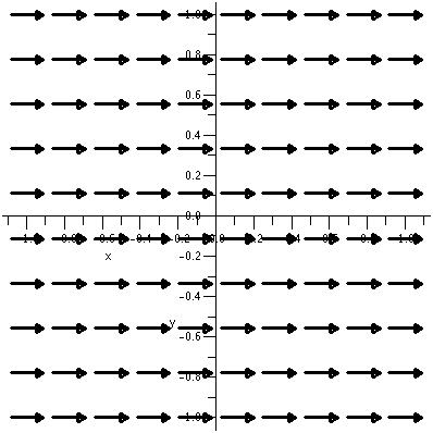
|
|
3xi+0j, a flow which doesn't move on the y-axis, but
flows away from the y-axis otherwise, and faster, the farther the
fluid was away from the axis.
| 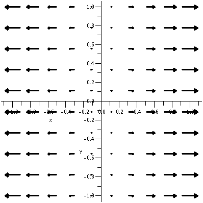 |
|
Associated to a fluid flow are streamlines, which would describe how a fluid
actually flows (the velocity vector field only would give what's called the
"instantaneous" flow). Such streamlines are investigated and can
sometimes be described exactly by solving differential equations.
So, what is a vector field?
- Geometrically, a vector field "is" a collection of arrows in the
plane.
- Algebraically, a vector field "is" a pair of functions,
f(x,y)i+g(x,y)j.
HOMEWORK
Please read about cylindrical and spherical coordinates and begin
reading chapter 16, at least 16.1 and 16.2.
Hand in at the next recitation:
15.8: 8, 19; 16.2: 3, 11; hand in a plot of the vector field ((10/x)+x2)i+((10/y)+y2)j with 100 vectors in the region
1/2<x<5 and 1/2<y<5.
Hint Don't do this by hand!
|
| Not this kind of arrow! |
|---|
 |
| Identify the historical figure
and the painter and win BIG! |
|---|
|
Maintained by
greenfie@math.rutgers.edu and last modified 3/24/2006.