Math 251 diary, spring 2010
Much later material
Later material
In reverse order: the most recent material is first.
Monday, February 22, lecture #11
(first 25 minutes!)
As I mentioned in class, a goal of the QotD is to help me assess how
successful the lecture was. The last lecture didn't get this
assessment. Here is what I might have liked to use.
Leading up to the QotD
Suppose I have a function of two variables, f(x,y), and I know the
following information:
f(0,0)=A and (∂f/∂x)(0,0)=B and (∂f/∂y)(0,0)=C
and
(∂2f/∂x2)(0,0)=D
and (∂2f/∂x∂y)(0,0)=E
and (∂2f/∂y2)(0,0)=F
Now I will define a function g with a one-variable input by the
equation g(t)=f(4t1+5t2,6t3). 1 2 3 4 5 6 This is entirely absurd -- I just assigned
the powers and the coefficients in a direct way.
Some questions and some answers
- What is g(0)?
Since g(t)=f(4t+5t2,6t3), I know
g(0)=f(4·0+5·02,6·03+2)=f(0,0)=A.
- What is g´(0)?
Since g(t)=f(4t+5t2,6t3), I will use the
Chain Rule and the fact that f is differentiable in two
variables. That is,
g´(t)=(∂f/∂x)(4t+5t2,6t3)(4+10t)+(∂f/∂y)(4t+5t2,6t3)(18t2).
If we plug in t=0, then we get
g´(0)=(∂f/∂x)(0,0)(4)+(∂f/∂y)(0,0)(0)=4B.
- What is g´´(0)?
Well, this is a curious computation. I need to start with the
formula for g´(t). I don't care about g´(0): that's a
specific number and looking at it will not help me at all.
Since
g´(t)=(∂f/∂x)(4t+5t2,6t3)(4+10t)+(∂f/∂y)(4t+5t2,6t3)(18t2)
I need to consider how to differentiate things like
(∂f/∂x)(4t+5t2,6t3)(4+10t).
I will need the Product Rule, surely (this is a product). But the
first piece, (∂f/∂x)(4t+5t2,6t3), has
a strange function of two variable and so I will need to use
the Chain Rule for a two variable function. Let me try this piece
alone:
d/dt((∂f/∂x)(4t+5t2,6t3))=(∂2f/∂x2)(4t+5t2,6t3)(4+10t)+(∂2f/∂x∂y)(4t+5t2,6t3)(18t2)
When t=0 this is 4D+0E, just 4D. But this is only a piece of the
computation. It should be multiplied by (4+10t). And then there is the
other part of the Product Rule, and then there is the other term,
which similarly needs the Product Rule and the Chain Rule.
Here is, I hope, the correct formula for g´´(t):
((∂2f/∂x2)(4t+5t2,6t3)(4+10t)+(∂2f/∂x∂y)(4t+5t2,6t3)(18t2))(4+10t)+
(∂f/∂x)(4t+5t2,6t3)(0+10)+
((∂2f/∂x∂y)(4t+5t2,6t3)(4+10t)+(∂2f/∂y2)(4t+5t2,6t3)(18t2))(18t2)+
(∂f/∂y)(4t+5t2,6t3)(36t)
When t=0, many things drop out. The result is 16D+10B. I hope this is
what people got in class. Oh well, maybe 5 out of 85 people completed
this computation correctly.
The remainder of this lecture will be in the next
section of the diary. It won't be covered on the exam. Please
study.
Thursday, February 18, lecture #10
So let me review a little bit of what I should have covered
last time.
Directional derivative
If u is a unit vector, then the directional derivative of T at (x,y,z)
in the direction u is the rate of change of T at unit speed in the
direction u (at the point). The textbook's notation for this is
DuT(x,y,z) and the preceding discussion should convince you
that the directional derivative's value is ∇T(x,y,z)·u.
So suppose you are looking at the function
Q=x3w+zy2–2z. When x=1 and w=3 and y=2 and z=–1,
Q's value is 133+(–1)22–2(–1) which is
2–4+2=0. Isn't that nice? Maybe, but suppose I have the
task of trying to increase this function as much as possible, with the
restriction being that the square root sum of the squares of the
changes should be at most, say, .01 (maybe there is a restriction on
various kinds of costs or material or ...). What should be done?
The gradient of this function is a 4-dimensional vector with
components (x, y, z, w derivatives in order) 3x2w and 2zy
and y2–2 and x3. When x=1 and w=3 and y=2 and
z=–1, this is the vector ∇Q=<9,–4,2,1>: the gradient
vector. A unit vector in this direction is this vector divided by
sqrt(102). The direction of this vector is the direction of greatest
increase. That direction is
<9/sqrt(102),–4/sqrt(102),2/sqrt(102),1/sqrt(102)>. If I want
something whose length is .01 which will likely increase the value of
the function the most, I would bet on
<.01[9/sqrt(102)],.01[–4/sqrt(102)],.01[2/sqrt(102)],.01[1/sqrt(102)]>.
This is definitely too computational. Let me try a
differentiation problem which is more conceptual. It resembles some
calc 1 computations, but things will get more complicated soon.
A sphere problem
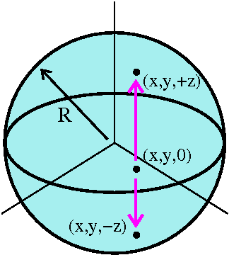 The points in R3 which satisfy
x2+y2+z2=R2 are a sphere
of radius R centered at (0,0,0). We could say that z is defined as a
function of x and y by this equation. In fact, since the situation is
relatively simple, we can actually solve for z in terms of x
and y:
z=±sqrt(R2–x2–y2). From
this equation we can compute ∂z/∂x etc. But if we assume
that z is defined implicitly as a function of x and y by the
equation, we can compute using the Chain Rule by just
∂/∂x'ing the whole equation:
x2+y2+z2=R2
becomes
2x+0+2z(∂z/∂x)=0 so
∂z/∂x=–2x/2z.
Some of the details of this computation need explanation. The
derivative with respect to x of x2 is certainly 2x. What
about the next term, the 0? x and y are independent
variables, and there is no way a change in x can force changes in
y. So here ∂y/∂x is 0. (The notation in this subject is
notoriously unhelpful -- you must keep track of the logical meaning of
the symbols.) And the Chain Rule applies to z2: we are
assuming that z is a differentiable function of x and y, so we
apply the Chain Rule to the square of this unknown function, and the
result is twice the function multiplied by the function's
derivative. Last, on the right-hand side of the equation,
R2, in spite of its appearance, is a constant and therefore
has derivative equal to 0. We take the resulting equation and "solve"
for the desired ∂z/∂x.
A more complicated example
The computations can be intricate. Let me try to write something quite
irritating:
Suppose z is implicitly defined as a function
of x and y by the
equation
z2sin(x+y2)+z3x=5ezy.
Find a formula for ∂z/∂y.
What I'll do is ∂/∂y the whole equation
carefully. Here x and y are independent, so ∂x/∂y is
0. The differentiation is a wonderful (?) example of expression
swell. I'll use zy instead of ∂z/∂y so I can
write less:
2z(zy)sin(x+y2)+z2cos(x+y2)(2y)+3z2(zy)=5ezy(zyy+z)
Let me try to analyze this intricate computation: for the
z2sin(x+y2) term I use the Product Rule followed
by the Chain Rule on each of the factors. I use the Chain Rule on
z3x and realize that x is a "constant" for this
computation. On the other side, 5ezy needs first the Chain
Rule, and then the Product Rule on its "argument", zy. The game now is
to "isolate" and solve for zy in this mess. Let me rewrite
the equation:
2z(zy)sin(x+y2)+z2cos(x+y2)(2y)+3z2(zy)=5ezy(zyy+z)
Maybe that typographical change helps. So I rewrite:
zy(2z sin(x+y2)+3z2)+z2cos(x+y2)(2y)=zy(5ezyy)+5ezyz.
Now I get, after some rearranging and a division: (–z2cos(x+y2)(2y)+5ezyz)
zy= ------------------------
(2z sin(x+y2)+3z2–5ezyy)
What a mess! This computation has no extra redeeming social value -- it is what it is.
More abstractly ...
I could analyze a function of two variables defined by using a
function of one variable (!?). O.k., here is what I mean: suppose I
have a function f with one variable input and one variable output. So
maybe we could write f is f(w), where w is a number. I could define
F(x,y)=f(x2+y2) and then try to compute, say,
both ∂F/∂x and ∂F/∂y. Since I don't know much
about f, when I need to differentiate it I just will write f´ and
try to go on. So here we go:
∂F/∂x=f´(x2+y2)2x.
∂F/∂y=f´(x2+y2)2y.
But then y∂F/∂x–x∂F/∂y=0
because the f´'s
cancel. So if I wanted to solve the partial differential
equation y∂F/∂x–x∂F/∂y=0 I have a collection of
solutions:
sin(x2+y2) and
ex2+y2 and
56(x2+y2)332 are all solutions.
Since such equations arise often in practice, this is nice.
A more significant example
 If we take a long "homogeneous" rope, and wiggle it a bit, the wiggles
propagate down the rope. It turns out (neglecting units,
neglecting certain other hypotheses, but keeping the central idea)
that for small wiggles, if we define f(x,t) to be the height of the
rope at position x and at time t, then
∂2f/∂x2=∂2f/∂t2.
This is called the one-dimensional wave equation. I can tell
you about all of the solutions. Suppose L and R are both
functions of one variable. Then define f(x,t)=L(x+t)+R(x–t). I'm not
going to tell you anything about the functions L and R except that
they are differentiable. Then the Chain Rule again applies:
∂f/∂x=L´(x+t)(1)+R´(x–t)(–1)
and further
∂2f/∂x2=L´´(x+t)(12)+R´´(x–t)(1)2.
 No, I don't really need to "write" the 1's
but I want you know that
they are there: the Chain Rule was used. Now again:
∂f/∂t=L´(x+t)(1)+R´(x–t)(–1) and further
∂2f/∂t2=L´´(x+t)(1)2+R´´(x–t)(–1)2.
And clearly (no!) f(x,t) satisfies
the Wave Equation. The names of the two functions, L and R, were chosen
because they model the movement of two "waves", a wiggle to the Left and a wiggle to the Right. I attempted to show this in class but was
frustrated because, first, the bungee cords were too darn springy --
in the wave equation's setup, there is no distortion due to internal
springs, and, second, there was reflection of the waves from the
ends. It is possible to analyze waves with reflections, but more
complicated than the setup I described, which is for an "ideal"
infinitely long string.
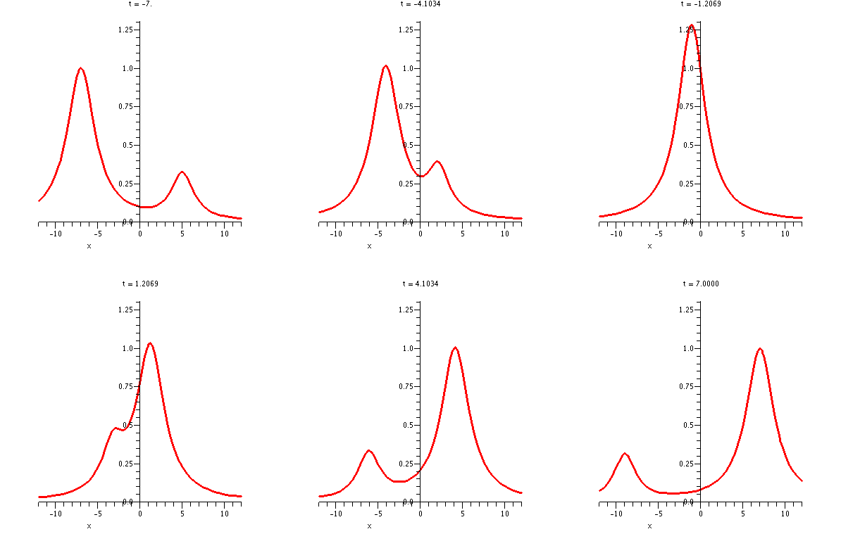
To the right is a picture created by Maple of the function
f(x,t)={1/(1+.25(x–t)2)}+{.3/(1+.4(2+x+t)2}. The
picture shows this function over the interval [–12,12] on the
x-axis, and t varies from –7 to 7. The picture was created using
the animate command.
The wave
traveling to the right has profile given by R(v)=1/(1+.35v2) and the wave
traveling to the left has profile given by
L(v)=.3/(1+.4(2+v)2). I hope you enjoy watching them.
|
Why?
All this is not intuitively obvious, at least to me. I bet that
some engineers and physicists would assert that the equation is
intuitive and clear. The equation turns out to be a very good model of
physical vibrations, for at least small displacements (just like
Hooke's Law does describe springs, but not if you try to stretch an
ordinary rubber band 10 feet!). Here are two links to reasoning which
shows how this equation follows from physical ideas:
At the University of
British Columbia This uses Newton's Law and force considerations.
A
Wikipedian entry This uses Newton's Law and Hooke's Law more
directly.
The two-dimensional wave equation is
∂2f(x,y,t)/∂x2+∂2f(x,y,t)/∂y2=∂2f(x,y,t)/∂t2.
It describes vibrations in thin plates.
The three-dimensional wave equation is
∂2f(x,y,z,t)/∂x2+∂2f(x,y,z,t)/∂y2+∂2f(x,y,z,t)/∂z2=∂2f(x,y,z,t)/∂t2
describes vibrations in solid objects.
It is much more difficult to find simple interesting solutions for the
two and three dimensional equations than for the one-dimensional
equation.
|
Crazy computations in thermodynamics and physical chemistry
I wanted to briefly indicate some horrible computations which come up
in applications. The computations are not really horrible, but the
notation makes them look quite weird. First, a bit of preparation.
If we have F(x,y) and both x and y are functions of one variable v (so
x=x(v) and y=y(v)), then what happens if we try to differentiate F
with respect to v? So basically we have, say, g(v)=F(x(v),y(v)), and I
want to understand g´(v). The control from v to F's output
is passed through two variables. I remember that
F(x+Δx,y+Δy)≈F(x,y)+(∂F/∂x)Δx+(∂F/∂y)Δy.
so that
F(x+Δx,y+Δy)–F(x,y)≈(∂F/∂x)Δx+(∂F/∂y)Δy.
If I now divide by Δv, we get
ΔF/Δv≈(∂F/∂x)(Δx/Δv)+(∂F/∂y)(Δy/Δv).
If I take limits as Δv→0, then this formula appears:
g´(v)=(∂F/∂x)x´(v)+(∂F/∂y)y´(v).
This is another "Chain Rule" and the weird thing about it is the
+ which comes from the definition of differentiability in
several variables. So let me show you some applications.
Implicit functions, two dimensions
I first began with a
return to a 1 variable calculus situation:
Suppose F(x,y) is a differentiable function of 2 variables, and the
equation F(x,y)=0 defines y implicitly as a function of x. What
is dy/dx in terms of F and "things" related to F?
So take the equation F(x,y)=0 and d/dx this equation. The right-hand
side is 0, and the left gives you:
∂F/∂x(dx/dx)+∂F/∂y(dy/dx) by the chain rule.
Certainly dx/dx is 1, and dy/dx is what we want, so we can "solve" for
it in the equation ∂F/∂x+∂F/∂y(dy/dx)=0. This
means:
A formula!
dy      ∂F/∂x
-- = – -------
dx      ∂F/∂y
Example
I think an example is needed here before we go on. Let's look at a
Calc 1 problem:
Find dy/dx if
y3–7xy2+4x5–6=0.
Calc 1 solution to Calc 1 problem
We d/dx everything, being careful to remember that y=y(x)
mysteriously. Then:
3y2y´(x)–7y2–(7x)2yy´(x)+20x4=0,
and now we solve for y´(x). We get:
y´(x)(3y2–(7x)2)–7y2+20x4=0 so that
y´(x)=–(–7y2+20x4)/(3y2–(7x)2).
New technology (?) solution to Calc 1 problem
We will use the formula above. Here
F(x,y)=y3–7xy2+4x5–6 so that
∂F/∂x=–7y2+20x4 and
∂F/∂y=3y2–(7x)2y+0 and the formula gives
dy/dx=–(∂F/∂x)/(∂F/∂y)=–(–7y2+20x4)/(3y2–(7x)2y+0)
which is of course the same answer! And you can look at see the same
pieces occurring, so the world is not so crazy.
The darn formula, though, is a bit mysterious. If you try to
understand the form (?) of the formula, the ∂x and ∂y might seem in
the wrong place and there might be an extra minus sign ... and ... and
... the notation is terrible!
P and V and T
Do you know about gas laws? For a gas, there are the
quantities P (pressure) and V (volume) and T (temperature). A gas
law might be a function of three variables which relates these
quantities:
G(V,P,T)=0.
If we assume that the function is differentiable and that each one of
the quantities is implicitly defined as a function of the other two by
the function, something funny happens. Let me show you.
Suppose that G(V,P,T)=0 implicitly defines V as a function of P and
T. Let's compute ∂V/∂P. Here T is constant, and sometimes in
thermodynamics the quantity is called (∂V/∂P)T just to
remind people that T is constant. We will ∂/∂V the equation
G(V,P,T)=0.
I use the chain rule, and the result is:
(∂G/∂V)(∂V/∂P)+(∂G/∂P)(∂P/∂P)+(∂G/∂T)(∂T/∂P)=0.
But ∂P/∂P must be 1 (the derivative of something with respect to
itself) and ∂T/∂P must be 0 (because T is constant!). Therefore we
can solve for ∂P/∂V just as we got dy/dx before and get:
∂V/∂P=–(∂G/∂P)/(∂G/∂V).
By the way, in applications people frequently change ∂V/∂P
to (∂V/∂P)T to help remember that T is constant
in this computation.
So far so good. But in fact we can find other partials in a similar
way:
∂P/∂T=–(∂G/∂T)/(∂G/∂P)
∂T/∂V=–(∂G/∂V)/(∂G/∂V).
Now clearly (NOT AT ALL
CLEARLY!):
(∂V/∂P)T(∂P/∂T)V(∂T/∂V)P=–1
because when we multiply all these expressions together the fractions
all cancel and we are left with –1. Why is this true physically
and what does it mean? Take physical chemistry, take thermo, etc.,
and find out. But the notation is horrible and, for me, makes things
harder to state and understand.
After class a few people expreseed doubts
about all this. So let me here try an explicit example. My "gas law"
will just be sort of silly and not physically meaningful.
Suppose P and V and T obey the following "law":
P2T+Ve3P+5T=0.
So the left-hand side of that equation is G(P,V,T). Now what is
∂V/∂P (with T held constant). So ∂/∂P the
equation. The result is
2PT+(∂V/∂P)e3P+5T+Ve3P+5T3=0. We solve
to get
∂V/∂P=–(2PT+Ve3P+5T3)/(e3P+5T).
Now I want ∂P/∂T (with V held constant). So ∂/∂T the
equation. The result is
2P(∂P/∂T)T+P2+Ve3P+5T{3(∂P/∂T)+5}=0.
We solve to get here
∂P/∂T=–(P2+Ve3P+5T5)/(2PT+Ve3P+5T3).
Finally, I will try to compute ∂T/∂V with P held
constant. We ∂/∂V the equation, and we get
P2(∂T/∂V)+1e3P+5T+
Ve3P+5T5(∂T/∂V)=0. Now solving gives
∂T/∂V=–(1e3P+5T)/(P2+Ve3P+5T5).
Now plug all this stuff into (∂V/∂P)T(∂P/∂T)V(∂T/∂V)P. Here we go:
(–(2PT+Ve3P+5T3)/(e3P+5T)
)(–(P2+Ve3P+5T5)/(2PT+Ve3P+5T3)
)(–(1e3P+5T)/(P2+Ve3P+5T5)
).
Check it out! Lots of things cancel, and we have
(–1)3=–1. YES!!!
|
A large part of the exam will ask about the material we discussed in
both of this week's lectures.
Monday, February 15, lecture #9
Exam warning!
Our first exam will be on Thursday, February 25. More information is
here. You also have a writeup
due tomorrow, there will be a quiz tomorrow, and a Maple lab started tomorrow, due in a
week. Lots of stuff!
The spaceship in a nebula
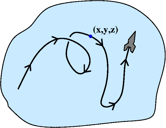 My online dictionary states that a nebula is "a cloud of gas
and dust, sometimes glowing and sometimes appearing as a dark
silhouette against other glowing matter." So we could pilot a
spaceship through a nebula. We might be concerned about the physical
effects of the nebula, for example, the temperature. I'll assume that
the spaceship measures temperature at the tip of its front. A point in
the nebula will be located with rectangular coordinates, (x,y,z). The
temperature at that point will be T(x,y,z). The rocket will fly a path
so that at time t its location will be <x(t),y(t),z(t)>.
From this we can see that the temperature measured at the rocket at
time t is T(t)=T(x(t),y(t),z(t)), and this is a composition. First we
find out where the spaceship is at time t, and then we compute the
temperature at that point.
Computing dT/dt
I would like to compute and understand the rate of change of the
temperature, T, with respect to time. It turns out that this is a
significant computation. Now T is a number and t is a number and T is
a function (complication: there are intermediate variables x, y, and
z) of t. So the derivative of T will involve taking its value at
t+Δt and looking for the linearization multiplier. That is what we declared earlier. So here we go. I will
try to accompany the steps of this somewhat elaborate manipulation
with explanations.
|
T(x(t+Δt),y(t+Δt),z(t+Δt))= |
|
|
We are "kicking" the time variable a little bit, and we would like to
examine the change in the T variable. |
|
T(x+x´(t)Δt+H.O.T.,y+y´(t)Δt+H.O.T.,z+z´(t)Δt+H.O.T.)=
|
| |
We use the fact that each of the components of the
position vector are differentiable, so each function value at
t+Δt can be replaced by the original value of the function, a
multiplier (the derivative) which multiplies the disturbance, and
higher order terms. If I were being careful, I would use different
notation for each of the H.O.T.'s, but in practice people don't do
that too often. You'll see why soon. |
|
T(x,y,z)+(∂T/∂x)(x´(t)Δt+H.O.T.)+(∂T/∂y)(y´(t)Δt+H.O.T.)+(∂T/∂z)(z´(t)Δt+H.O.T.)+H.O.T.
|
| | This is the differentiability of T. The
changes in the inputs to T (there are three inputs) are passed
outside. What happens? The linearization idea says that the changes
are each multiplied by an appropriate partial derivative. And this
isn't really exact (the numerical example
showed this!) so there is also a H.O.T. from the
differentiability of T. (Complicated? Sure is.)
|
|
T(x,y,z)+(∂T/∂x)(x´(t)Δt)+(∂T/∂y)(y´(t)Δt)+(∂T/∂z)(z´(t)Δt)+
(∂T/∂x)H.O.T.+
(∂T/∂y)H.O.T.+
(∂T/∂z)H.O.T.+
H.O.T.
|
| | Now I did some multiplication and
rearrangement. I pushed everything involving any of the Higher
Order Terms to the end. |
|
T(x,y,z)+(∂T/∂x)(x´(t)Δt)+(∂T/∂y)(y´(t)Δt)+(∂T/∂z)(z´(t)Δt)+H.O.T.
|
| |
Here is the important step, and it sort of asks you to think a bit
about the ideas of calculus. All of the terms with H.O.T. are
actually, all added together, just another big H.O.T.
|
|
T(x,y,z)+{(∂T/∂x)(x´(t))+(∂T/∂y)(y´(t))+(∂T/∂z)(z´(t))}Δt+H.O.T.
|
| | This is the last rearrangement. Please, I hope
you have the patience to see what has happened. We have the "old"
unperturbed value of T(x(t),y(t),z(t)), and then we have a mess (not
really, as you'll see) multiplying Δt, and then, finally, we
have a whole bunch of things which logically are inside the H.O.T. |
Now what? If f(v) is a function of one variable, then
f(v+Δv)=f(v)+f´(v)Δv+H.O.T.
identifies the derivative of f by what happens to small perturbations.
The red stuff is the derivative, because it is the multiplier of the
small perturbation of the input.
We carried out an elaborate analysis of how the temperature function
changes. Now look at the result again:
T(x(t+Δt),y(t+Δt),z(t+Δt))=T(x,y,z)+{(∂T/∂x)(x´(t))+(∂T/∂y)(y´(t))+(∂T/∂z)(z´(t))}Δt+H.O.T.
The multiplier of Δt is dT/dt, so we see that
|
dT/dt=(∂T/∂x)(x´(t))+(∂T/∂y)(y´(t))+(∂T/∂z)(z´(t))
|
|---|
But this formula is not the point of the discussion. Look at
the equation and think a bit. The
luck and glory is recognizing that the mess on the righthand
side is a dot product. In fact, look:
dT    / ∂T   ∂T    ∂T \    / dx   dy   dz \
-- =   --- , --- , ---  ·   -- , -- , --
dt    \ ∂x   ∂y    ∂z /    \ dt   dt   dt /
Left Right
There are certainly many ways to organize this as a dot product, but
this way turns out to give some insights that amaze me.
Right
The vector on the right-hand side is one we've looked at when
discussing curves. It is the derivative of r(t), the position vector,
so it is v(t), the velocity vector. This vector deals with the
spaceship and its motion.
Left
This vector seems to be "new": it is the vector of
all the first partial derivatives of T in order. This is called the
gradient of T and is frequently written ∇T and is
sometimes also called grad T. The upside-down triangle (or upside
down Δ) is sometimes called "del" or "nabla". This vector can be
computed only from the nebula information.
Thinking about the temperature derivative this way "decouples" (yeah,
a word that's used) the influence of the nebula from that of the
spaceship.
Now I will try to make a sequence of observations which might help people
understand the excitement I feel thinking about gradient.
Observation 1
Let's imagine two spaceship trips through the nebula. Now these
trips (voyages?) may be completely different except that at the
time the two spaceships pass through the point (x,y,z), the
spaceships have the same velocity vectors: that is, the spaceships are
heading in the same direction and at the same speed. Their v(t)'s are
the same. Then the rate of change of the temperature,
dT/dt, that the two spaceships measure is exactly the
same.
I asked students if they could deduce this from the physical and
geometric aspects of the "scenario". I don't think I can. As a math
fact goes, this is nearly obvious: since the v(t)'s are the same, the
right-hand side doesn't change, and the nebula's temperature function
is the same, so the left-hand vector ∇T doesn't change. Therefore
the dot product, which computes dT/dt, is the same. But ... but
... what the heck ... can you "see" this physically? This is not the
temperature at the point, but the rate of change of the
temperature: the rate of change is the same if the velocity vectors
are the same.
Observation 2
Now r´(t)=v(t), the velocity vector. Let me call the unit tangent
vector u(t) here (in the discussion of curvature it was called T(t)
but that will just be too darn confusing). Then v(t) is the same as
(ds/dt)u(t) where ds/dt is the speed and u(t) is the unit tangent
vector. In the formula ∇T·r´(t) the ds/dt effect just
"filters out" of the dot product. If you travel twice as fast on the
same path, then the rate of change of the temperature with respect to
time is just doubled. So this is easy to understand. But the more
subtle aspect is what happens as the direction changes.
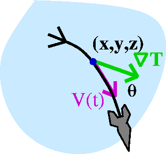 Observation 3
Here I will suppose that ds/dt=1 for simplicity.
Again, call the unit tangent vector, u, for unit
vector. Then what can we say about ∇T·r´(t)? It is
(ds/dt)∇T·u, or just (since I'm assuming unit speed)
∇T·u. But, hey, the dot product is also
||∇T|| ||u||cos(θ). Since cos(θ) is between –1 and +1, I
now know that dT/dt is between –||∇T|| and +||∇T||.
How could we choose u so that dT/dt is largest? We need to make
cos(θ) equal to +1. Therefore we need θ to be 0, and u should
be a unit vector in the direction of ∇T. That is, choose u to be
∇T/||∇T||. To make the rate of change as much negative as possible,
choose u to be –∇T/||∇T||, and then dT/dt will be –||∇T||.
An example (?)
Here is an example.
If T(x,y,z)=x2eyz–5z3 then since
∇T=<∂T/∂x,∂T/∂y,∂T/∂z>, we compute:
∇T=<2xeyz–5z3,x2eyz–5z3(z),x2eyz–5z3(y–15z2)>
As far as I know this function and this computation has no great or special
"meaning".
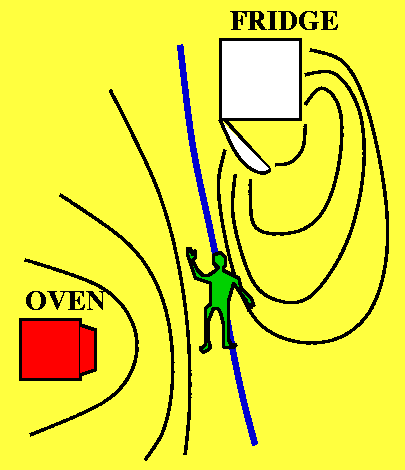 A better example (!)
Im my kitchen I have just finished baking my famous chocolate brownie
pie and I left the oven door slightly open. Also I managed to forget
to close the refrigerator. As a result, the contour lines of
temperature could like what is shown to the right. In what direction
should I go (I am the little green man in the picture!) to most
rapidly increase the temperature? In the direction of the gradient,
which will point towards the oven. I will most rapidly decrease the
temperature by traveling in the opposite direction, towards the source
of the cold.
Observation 4
I could imagine that spaceship travels through the nebula on an
isothermal surface. An isothermal is a collection of points
where the temperature is all the same. We have seen this already:
T(x,y,z)=C is a level surface (dimension 3) or level curve (dimension
2) or a contour {surface|curve}. But if the spaceship travels on such
a surface, then the rate of change of the temperature must be 0. But
then ∇T·v=0. This means that the velocity vector is perpendicular
to the gradient. But then in turn this means that the gradient vector
is perpendicular to the level surface, and it is perpendicular to the
tangent plane of the level surface. In the kitchen, I would walk
perpendicular to the contour lines to increase or decrease
temperature most rapidly. I would walk along the contour lines if I
wanted no rate of change of temperature.
Back to the example
Let me look more closely at the example with
T(x,y,z)=x2eyz–5z3
when x=3 and y=2 and z=1. Then T(3,2,1)=9e–3. And
∇T=<2xeyz–5z3,x2eyz–5z3(z),x2eyz–5z3(y–15z2)>
becomes
∇T(3,2,1)=<6e–3,9e–3(1),9e–3(–13)>=<6e–3,9e–3(z),–117e–3>
Now forget all that, and solve the following
geometric problem:
What is the equation of a plane tangent to the surface
x2eyz–5z3=9e–3 at the
point (3,2,1)?
This could be, indeed, I claim, this is a hard problem. But if
we now disobey my urging ("forget all that") I can tell you that
∇T(3,2,1) is perpendicular to the surface and to its tangent plane
at (3,2,1). So I can write the answer, since I know a point and a
normal vector to the plane requested:
6e–3(x–3)+9e–3(y–2)+–117e–3(z–1)=0.
I think that solving such a problem so efficiently is really remarkable.
Another example
Suppose I want an equation for the plane tangent to
z=3x2+5xy2 when x=1 and y=2. Well (curious
trick!) if I consider T(x,y,z)=3x2+5xy2 z then
the surface z=3x2+5xy2 is exactly the
isothermal or level surface corresponding to T=0. Now ∇T
will be perpendicular to that surface. We compute:
∇T=<6x+5y2,10xy,–1>. We know that x=1 and
y=2 so that the gradient is <26,20,–1>, which is a vector
perpendicular to the plane. Now we need a point on the surface. But we
know z=3x2+5xy2 and x=1 and y=2 so we can deduce
z: z=23. A point on the plane is (1,2,23). Therefore an equation for
the tangent plane is
26(x–1)+20(y–2)+–1(z–23)=0.
Here is another way we could get the tangent plane. I could have done
this last time, but the gradient is just a simpler way to get the
result.
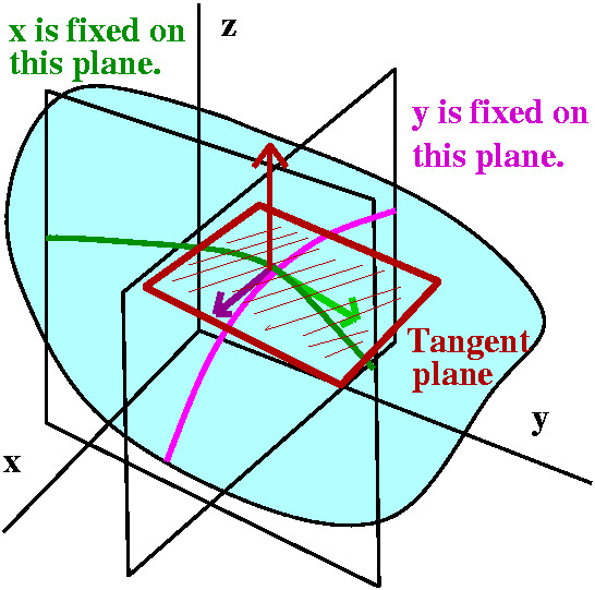 Tangent planes
We can get a bit more out of the slicing picture. The vector i+∂f/∂xk is tangent to the curve in
R3 gotten by fixing y on the surface z=f(x,y), and the
vector j+∂f/∂xk is tangent to the curve in
R3 gotten by fixing x on the surface z=f(x,y). If the
surface is nice and smooth (that is, if the function f(x,y) is
differentiable) people agree that the two vectors determine a plane
which is tangent to
y=f(x,y). To write the equation of a plane, we need a point and a
normal vector.
Suppose we're at the point
(x0,y0,f(x0,y0)). The
normal vector will be perpendicular
to both i+∂f/∂x(x0,y0)k and j+∂f/∂x(x0,y0)k. So we need
to compute the cross product:
[i+∂f/∂xk]x[j+∂f/∂xk]. So:
   ( i  j     k )
det( 1  0  ∂f/∂x)=–[∂f/∂x]i –[∂f/∂y]j +k=a normal vector
   ( 0  1  ∂f/∂y)
Then if you remember the data needed to write a plane (a point and a
normal vector) we can write the equation of a tangent plane.
An equation for a tangent plane
If f(x,y) is differentiable, then the equation of a plane tangent to
z=f(x,y) when x=x0 and y=y0 is
(z–z0)=∂f/∂f(x0,y0)(x–x0)+∂f/∂y(x0,y0)(y–y0).
Example
Find the equation of a plane tangent to
z=3x2+5xy2 when x=1 and y=2.
Here z=3+5·22=23. Now for the derivatives:
zx=6x+5y2 and this is 26 when x=1 and y=2;
zy=10xy and this is 20 when x=1 and y=2;
The tangent plane equation
(z–z0)=∂f/∂f(x0,y0)(x–x0)+∂f/∂y(x0,y0)(y–y0)
becomes (z–23)=26(x–1)+20(y–2).
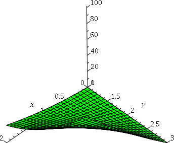
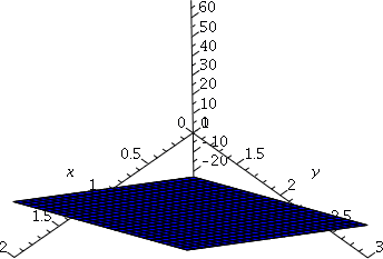
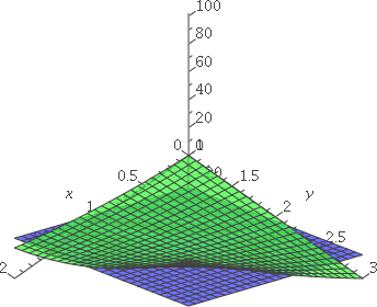
Below are some pictures generated by Maple. The third, showing both the surface and
the tangent plane, is a bit hard to understand. The surface bends
below the plane in one direction, and above in another
(very "saddle-like").
| The surface near (1,2,23) |
The plane near (1,2,23) |
Both near (1,2,23) |
 |
 |
 |
|
Topographic maps
A topographic map shows contour lines. Frequently while hiking people
mind want to find the most direct route to the "top" (a mountain peak)
or to the "bottom" (a creek?). They know by experience that the most
direct route, only looking at the map, that is, only the geometry of
the situation, would be to walk as nearly as possibly perpendicular to
the contour lines.
This can be adapted into computational strategies for finding
maxes and mins. If you can readily compute your function's gradient,
then find maximums by going in the direction of the gradient. This is
hill climbing. Find minimums by going opposite the direction of
the gradient. This is the method of steepest descent. Of course
these computational ideas don't always work, and there are many
implementation details to worry about, but the general strategy is
valuable.
Contour map example
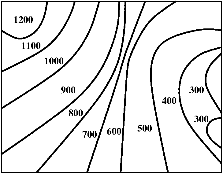
So to the right is a made-up example of a contour map. The lines
shown are at height multiplies of 100 feet. I hope that you can
see (?) there is sort of one part of the map which deserves the
name "peak" (in the upper left-hand corner). This map is a bit more
complicated than the one I drew in class. I claim there is also a part
of the map which could be named "the pits" (probably at least two of
them!) and that's inside the two loops at the 300 foot height.
|  |
Hill climbing -- a way to get to the maximum
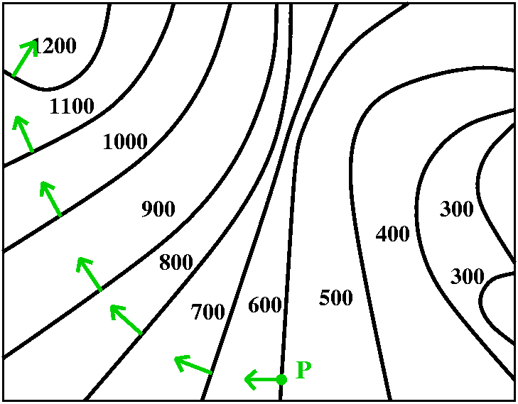
Now suppose we are at the point P on the
map. How should we hike in order to get uphill as fast as possible? I
claim that the directions shown will do that. Notice that I am
not always walking towards "the peak", but I just want to
always walk perpendicular to the contour lines -- in the direction of
the gradient of the height function.
|  |
The method of steepest descent -- how to get to the minimum
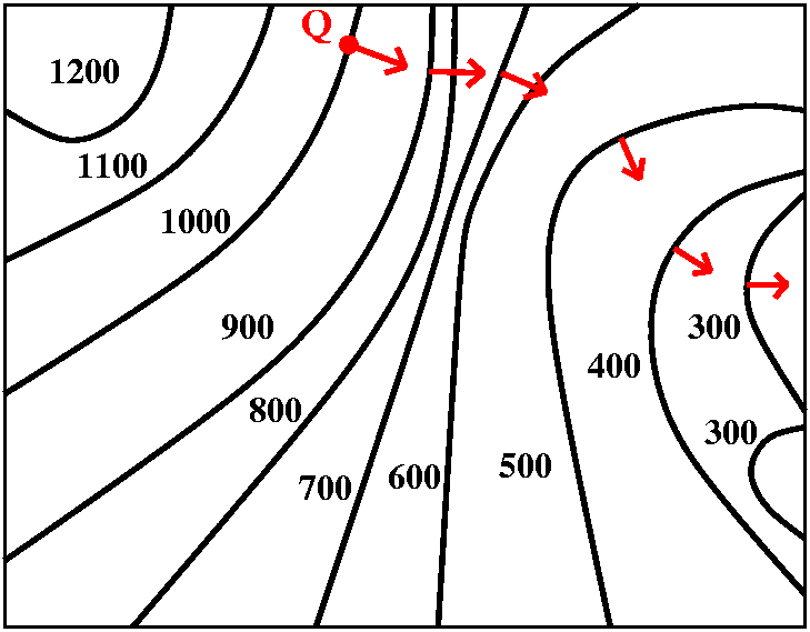
This is a way people use to try to get to minima of functions in
several variables. We start at the point Q and
move in the direction opposite the gradient of the height function. In
what I'm showing here, we take some sort of fixed step size (more
sophisticated versions vary the step size) and after that step we keep
going until we hit another contour line. Then we recompute the
direction (minus the gradient) and step again. You can see, I hope,
that this path is headed for one of "the pits".
These methods don't always work and don't always work efficiently, but
they are easy to understand, they can be done in many dimensions, and
the programs run fast.
|  |
The most change
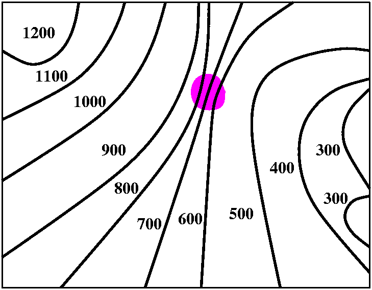
I could also ask where there is the most change in
height in a fixed distance. These are contour lines
corresponding to equal changes in height. The heights will change most
rapidly (as a function of the position on the map) when the contour
lines are most closely spaced. This also corresponds, of course, to
the region in the plane where ||∇ height|| is largest: the
largest magnitude of the gradient vector. I think the region indicated
(in magenta) is the region in this rather simple contour chart.
|  |
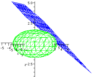 The QotD: tangent plane to an ellipsoid
Here's a neater example. Consider the ellipsoid (egg)
x2+2y2+3z2=9. The point (2,1,1) is on
this ellipsoid. What is the equation of a plane tangent to the
ellipsoid at (2,1,1)? The gradient of the function
x2+2y2+3z2 is <2x,4y,6z> and at
(2,1,1) this is <4,4,6>. The equation of the tangent plane is
4(x–2)+4(y–1)+6(z–1)=0.
To the right is a Maple picture made by
the commands which
follow. I hope that the picture helps to convince you that the plane
is the tangent plane.
A:=implicitplot3d(x^2+2*y^2+3*z^2=9,x=-5..5,y=-5..5,z=-5..5,grid=[20,20,20],
axes=normal,labels=[x,y,z],color=green,style=hidden);
B:=implicitplot3d(4*(x-2)+4*(y-1)+6*(z-1)=0,x=-5..5,y=-5..5,z=-5..5,axes=normal,
labels=[x,y,z],color=green,style=hidden);
display({A,B};
I forgot to mention this definition. Please forgive
me!
Directional derivative
If u is a unit vector, then the directional derivative of T at (x,y,z)
in the direction u is the rate of change of T at unit speed in the
direction u (at the point). The textbook's notation for this is
DuT(x,y,z) and the preceding discussion should convince you
that the directional derivative's value is ∇T(x,y,z)·u.
more notation, more words ... this is so
terrific!!! (so academic)
|
Thursday, February 11, lecture #8
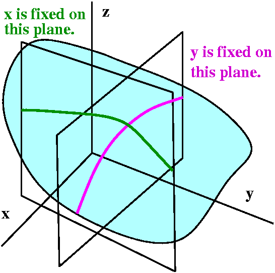 Slicing and partial derivatives
Now we can define partial derivatives. Please realize that everything
we are doing can be done in any number of variables (want a
picture of 703 dimensions?) but I'll stick with 2 dimensions here
because I can draw pictures and I like pictures.
So look at a graph of z=f(x,y). We can slice this in various ways. For
example, we could slice this by a plane
perpendicular to the y axis with y fixed. This will give sort
of an z-x curve. We could "lift" that curve up and just consider it as
a function of one variable, x, and then look at the derivative. That's
∂f/∂x. This notation, with a sort of curly d, is not
terrific, and it can be (as we will see) quite confusing. But it is
what almost everyone uses. Similarly, we could slice by a plane perpendicular to the x axis with x fixed
and consider the derivative of the resulting curve or function. That
will be ∂f/∂y. Here are the formal definitions if you would
like them:
limh→0(f(x+h,y)–f(x,y))/h=∂f/∂x
limk→0(f(x,y+k)–f(x,y))/k=∂f/∂y
|
I'll use h for little changes in the first variable and k for little
changes in the second variable.
I did some silly examples and then actually computed some partial
derivatives (∂/∂t and ∂2/∂x2)
of F(x,y)=e–x2/(4t)/sqrt(t). This
function occurs in many applications analyzing diffusion, including
heat and fluid mixing. Let's see:
- ∂F/∂t=e–x2/(4t))(–x2(–t–2/4)/sqrt(t)+e–x2/(4t)(–1/2)t–(3/2).
This is e–x2/(4t) multiplying
x2/(4t5/2)–1/(2t3/2)
- ∂F/∂x=e–x2/(4t)(–2x/(4t))·(1/sqrt(t))
which is e–x2/(4t)(–x/(2t3/2)).
- ∂2F/∂x2=e–x2/(4t))(–2x/(4t))(–x/(2t3/2))+e–x2/(4t))(–1/(2t3/2)). This is
e–x2/(4t)) multiplying
(–2x/(4t))(–x/(2t3/2))+(–1/(2t3/2)). The
second factor is x2/(4t5/2)–1/2t3/2.
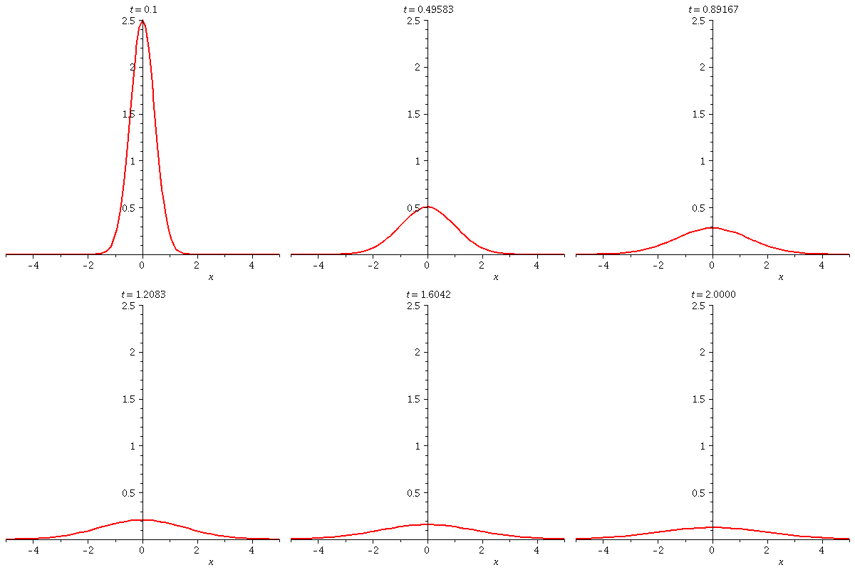 So F is a solution of the Heat or Diffusion Equation
∂F/∂t=∂2F/∂x2
This is the one-dimensional version of the equation, and describes how
temperature changes over time, t, at position x in, say, a thin
homogeneous rod. Similar but more complicated equations describe
what's happening in a plate or a solid object, or how fluids diffuse
(heat and fluid diffusion have very similar mathematical
descriptions). There are more than three and a half million Google links for the phrase "heat equation".
To the right is an animation of the temperature for time ranging from
t=.2 to t=2. Near .1, a bunch (??) of heat is injected into the bar at
x=0 (strike a match, etc.). I started the picture a bit later than 0,
because the match is infinitely hot (?) at t=0. The amazing thing is
that this function does describe or model a real situation nicely. The
heat diffuses quite rapidly. Please note that I have not
mentioned units either here or in the lecture. This was intentional,
although the situation does get distorted a bit. The units etc. can
get quite complicated.
A betting game (?)
Consider this situation: suppose f(x,y)=(sin(y4)x–7)3. Then I flip a (fair) coin. If it lands
"heads", I ∂/∂x this function. If the coin shows "tails", I
∂/∂y the function. What's going to happen? I asked students
to speculate about this. Almost everything that students said was
correct. I sometimes tried to distract people from the real question
by making interesting and true assertions. For example,
∂100f/∂y100 yields a mess with 342
terms. And 200 y derivatives gives an algebraic mess with 680
terms. These computations were not done by hand, but with Maple. The expressions begin to swell
(get larger and larger). I asked students if they thought that this
sort of growth would be likely under the conditions of the
experiment. Some students kept remarking about ∂/∂x and I
kept "distracting" with facts about ∂/∂y. Here is an
important and relevant result for this game.
Clairaut's Theorem (equality of "mixed" partial derivatives)
Suppose f(x,y) is a function of two variables, and the mixed partial
derivatives fxy and fyx both exist and are both
continuous. Then these mixed partial derivatives must be the same.
Certainly in Math 251, the hypotheses of the theorem will be
satisfied. There are examples (similar in nature to the bizarre
functions previously given) where things aren't the same. But in this
course, the mixed partials will be continuous and therefore will
agree. The verification of this result is in the textbook and uses the
Mean Value Theorem of 1 variable calculus (you sort of take two double
differences and analyze them, much as the differences in rows and
columns of a spreadsheet). As I said, this result will apply to almost
all functions we will meet in 251. The result implies, for example,
that if we look at the "crowd" of all the possible third partial
derivatives of a function of two variables:
fxxx fxxy fxyx fyxx fxyy fyxy fyyx fyyy
it may seem that there are eight possibilities. But due to Clairaut,
there are only these four:
fxxx fxxy fxyy fyyy
The effect of the "concentration" gets even stronger as the number of
derivatives increases.
Return to the game
How does Clairaut influence my original question? Again, I was perhaps
not the most helpful person in leading the discussion, but eventually
the most relevant fact appeared. The function f(x,y)=(sin(y4)x–7)3 is a cubic (degree 3) polynomial in
x. That is, it can be written as
(Stuff0)x0+(Stuff1)x1(+Stuff2)x2+(Stuff3)x3
where each of the "Stuff" terms is some function only involving y. An
x derivative, ∂/∂x, lowers the degree in x. And four x
derivatives will leave us with 0. If you toss a coin a large number of
times, it is overwhelmingly likely that there will be at least 4
heads, and therefore, in the differentiation choices, at least 4 x
derivatives. So since we can reorder these mixed partials in any way
we want, we could put those four derivatives first. And the result
will be 0. So, almost surely, if we toss a coin many times, and follow
the directed sequence of derivatives, the result will be 0.
What does differentiable mean in 1 variable?
What does f´(x)=Q mean? The definition we all tried to memorize
(for a while, anyway) went something like this:
This definition is difficult to compute with because it has division
and subtraction. People frequently "unroll" it to the following:
Here f(x) is the old, unperturbed output or response of f to the input
of x. We perturb (kick?) the function box with a small w. The response
of f to x+w can be decomposed (if f is
differentiable!) into f(x), the old response, a linear or first-order
disturbance, Qw, and "Error". The Error term is very complicated. Of
course it will depend on f and x and w (and maybe the phase of the
moon). But what is most important about the error term
computationally is that it approaches 0 faster than first
order. Frequently in applications the Error term is thought of or
labeled, H.O.T. for "higher order terms". A function is differentiable
in one variable exactly when its response to a small kick can be
described as above. This corresponds geometrically to a well-known
phenomenon that can be demonstrated nicely using graphing
calculators. If you take a point on the graph of a
differentiable function and zoom in repeatedly on the graph
(centered at the point) within usually a few "zooms" the graph begins
to look like a straight line (this is certainly not true of
f(x)=|x| at x=0!). Therefore the graph of y=f(x) is (approximately)
locally linear exactly when the function is differentiable. It is the
property of being approximately locally linear which turns out to be
important in higher dimensions. The derivative is the
multiplier effect of a small change in the input.
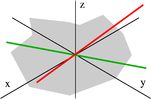 A really silly (?) two-variable example
I gave a very artificial example to show that things can be quite
strange in more than 1 variable. I defined a function, f(x,y) to be 2x
if y=0, 3y if x=0, and 0 otherwise. To the right is an effort to show
the graph, z=f(x,y), of this strange function. The green line is
supposed to be tilted above the x-axis (the tilt or slope is 2), the
red line is tilted 3 over the y-axis, and the remainder of the graph
is flat at z=0, the xy-plane.
Certainly if you slice the graph by y=0 (this is called a vertical
trace in the textbook) then you get z=2x, and the partial derivative
of f with respect to x exists and is 2. That is,
∂f/∂x(0,0)=2. Similarly, if you slice the graph by x=0 then
you get z=3y, and the partial derivative of f with respect to y exists
and is 3. That is, ∂f/∂y(0,0)=3.
This is a seriously silly function, but let me analyze it from the
point of view of differentiability at the point (0,0). Suppose that h
is a small perturbation in the first coordinate and k is a small
perturbation in the second coordinate. I would like to understand
f(0+h,0+y) in terms of the unperturbed value of f (that is, f(0,0)=0)
and also the first-order part (this should be ∂f/∂x(0,0)h=2h
and also ∂f/∂y(0,0)k=3k). So I ideally would like
f(0+h,0+y)=f(0,0)+2h+3k+H.O.T.
But look: what if both h and k are not both 0? Then we are on
the grey part of the graph, and the equation above becomes
0=0+2h+3k+H.O.T. whenever h and k are not both 0. We also want
H.O.T. to be truly "higher order" so it might have stuff like
h3/2 or k2 or even a combined higher order term
like hk. None of these will cancel out the 2h+3k. This extremely silly
(but rather simple) function does not have the approximation property
which we would like in differentiable functions. And it is this
approximation property which is needed in many applications -- this is
not "theory".
Repeating, looking at slices is not good enough to consider
limits and continuity. Slices, even collections of slices in two
perpendicular directions, just do not contain enough
information about the function. In the case of f(x,y) and its partial
derivatives, the key idea, both abstractly and computationally, turns
out to be the two dimensional analog of (approximate) local
linearity. If we "kick" the input to f in both x and y, we need to
understand how the function "responds". The nicest response, similar
to one dimension, would be the unperturbed response, f(x,y), then
something proportional to h plus something proportional to k, and,
finally, a higher-order error term.
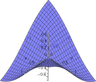 By the way, if you don't like piecewise defined functions, you could
consider the function defined by this formula:
f(x,y)=xy/sqrt(x2+y2). It has properties which
are similar to the piecewise function, but it is a bit harder to
analyze. You could look at it using Maple, and then you might get some insight.
The partial derivatives of this function are 0 at (0,0), so one might
expect and hope that the linear perturbation near (0,0) would be 0
*because both Constant1 and Constant2 are
0. But, in fact, if we increase x and y both by the same about (so
change x from 0 to 0+tiny and y from 0 to 0+tiny, then the resulting
value of f is exactly tiny, and this is first order and is not
0. This function is not differentiable at (0,0) even though both
partial derivatives (tangent lines to the curves in the slices!) exist
there: an irritating example. There is no local linearity at the
origin -- no matter how much you magnify it, the "surface" looks more
and more like a sort of cone, not like a piece of a plane.
|
Differentiable in two variables
In mathematics, when something is wrong, one way to help is by making
a definition. The functions we want to consider are called
differentiable and have exactly the property that they can be
approximated nicely.
f(x,y) is differentiable at (x,y) if there are numbers
Constant1 and Constant2 so that for h and k
small,
f(x+h,y+k)=f(x,y)+Constant1h+Constant2h+Error,
where the Error term→0 faster than |h|+|k| (so, faster than first
order -- it is H.O.T.).
Important results
Before hysteria strikes, here are two results which are verified in
the text. They are not difficult to check (again, the essential key is
the 1-variable Mean Value Theorem), but we just don't have time in
class.
Theorem If f(x,y) is differentiable, then the partial
derivatives of f(x,y) exist, and
Constant1=∂f/∂x(x,y) and
Constant2=∂f/∂y(x,y).
Theorem If ∂f/∂x and ∂f/∂y are both
continuous then f(x,y) is differentiable (in the approximation
sense defined above).
Please realize that essentially all functions we will meet in Math 251
will satisfy the hypotheses of the preceding theorem, so these
functions will be differentiable and will have suitable
approximation properties. In fact, here is a sort of easy example,
although there is some computation involved.
Linear approximation: an example
Here we looked at something like
f(x,y)=sqrt(x4–y2+2xy–3). Notice that
f(2,3)=sqrt(24–32+2·2·3–3)=
sqrt(16–9+12–3)=4. This is an example in a calculus class, and it was
chosen so that f(2,3) was nice.
Then
∂f/∂x=(1/2)sqrt(x4–y2+2xy–2)–1(4x3+2y)
and
∂f/∂y=(1/2)sqrt(x4–y2+2xy–2)–1(–2y+2x).
We can evaluate these derivatives at (2,3):
∂f/∂x(2,3)=(1/2)(1/4)(4·23+2·3)=(38)/8
and ∂f/∂y(2,3)=(1/2)(1/4)(–2·3+2·2)=–2/8.
If we want a linear approximation to f(2.03,2.98), then we may
use the following formula:
f(2.03,2.98)≈f(2,3)+∂f/∂x(2,3)(.03)+∂f/∂y(2,3)(–.02).
Here the change in x from 2 to 2.03 means that h is .03 and the change
in y from 3 to 2.98 means that k is –.02. The linearized
approximation gives us 4+(38/8)(.03)+(–2/8)(–.02) which is
4.1475. The "true value" (up to 10 decimal places!) of f(2,3) is
4.147314409.
As I declared in class, in 1910 this would be nearly amazing!
Accuracy to almost 4 decimal places. But, yuh'see, we have programs to
compute this. The idea of linear
approximation is what will be important.
QotD
If f(x,y)=xy, find
∂f/∂x and ∂f/∂y.
The first one is easy: ∂f/∂x=yxy–1 (this is just
x to a "constant" power after all). For the first, the best way is to
rewrite the function using exp and ln: xy=(eln(x))y=e(y ln(x)) and then
∂/∂y of e(y ln(x)) is e(y ln(x))ln(x). This is a fine answer, or it can
be rewritten xyln(x).
Monday, February 8, lecture #7
We move on to one of the major topics of the course. The word
"several" is technical in mathematics, and means "more than 1". So we
will study functions whose domain is several real variables, and whose
range is inside the real numbers. We'll begin with an almost
ludicrously simple function: f(x,y)=x2+y2.
x2+y2
Here f(x,y)=x2+y2. This is a function defined by
a formula (essentially all of the functions we'll consider in this
course will be defined by formulas). The notation means that the input
to the function is an ordered pair of numbers, (x,y), and the output
is one number. Here the output for the ordered pair (–2,3) is 13.
Formalities: domain and range
The domain will be the collection (the "set") of all possible
inputs. Just as in calc 1, if the function is defined by a formula,
then the domain in this course will be all inputs for which the
function makes sense. The usual restrictions that will concern us
are:
- Don't divide by 0.
- Only square roots of non-negative numbers are allowed (same for
other even roots).
- Logarithms only for positive numbers.
These should all be familiar to you.
The range will be the collection of all possible outputs. You
may remember from calculus that while determining precise domains is
often possible but tedious, precise descriptions of ranges can be
quite difficult (this can involve exact determinations of max and min
values).
Here are some examples chosen to illustrate the likely possible
restrictions. I certainly did not have time to discuss all of these in
class.
| f(x,y)=x2+y2 |
|---|
Domain
I think all pairs (x,y) of real numbers, all of R2.
|
Range
Since squares are non-negative, certainly the values of this function
are non-negative. And f(0,0)=0, and f(sqrt(A),0)=A for A positive. I
am just verifying precisely that the range is all non-negative real
numbers.
|
| f(x,y)=1/(y–x2) |
|---|
Domain
So this example is chosen to illustrate the restriction about not
dividing by 0. The domain is
all pairs (x,y) of real numbers for which y is not equal to
x2. Geometrically, this means all points of R2
which are not on the parabola y=x2.
|
Range
0 isn't in the range (it isn't the reciprocal of any number). But
everything else is: check this by just looking at what happens to
(0,A), which gives 1/A for all non-zero A's.
|
| f(x,y)=sqrt(y–x2) |
|---|
Domain
So this example is chosen to illustrate the restriction about square
roots. The parabola y=x2 divides R2 into two
pieces. One piece contains, say, the point (3,4) ("below" the
parabola). This point has y–x2=4–32=–5<0, so
(3,4) is not in the domain of this function. The domain is the
"other" piece of R2 and also those points which are on the
curve y=x2.
|
Range
The range is all non-negative numbers. Again, to check this you could
look at what happens to (0,A) for A≥0.
|
| f(x,y)=ln(y–x2) |
|---|
Domain
I still must "throw out" the part of R2 which is below the
parabola. But here inputs to ln must be positive, so the domain
does not include the curve y=x2. The domain is all of the
points in R2 which are above the parabola.
|
Range
The range is the range of ln, which is all real numbers.
|
Kinds of graphs
| Let me return to the
simplest of the functions I just considered:
f(x,y)=x2+y2. There are various graphs which are
commonly used. Maybe the simplest is to consider the points (x,y,z) in
R3 which satisfy the equation
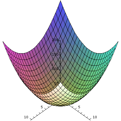
z=x2+y2: this is usually called the graph of
the function. A Maple representation
of this graph is shown to the right, and the procedure which produced
it is plot3d, part of the plots package. This is rather a simple
function, and I hope you can see the shape of this surface. It is a
cup, axially symmetric around the z-axis. It is called a
paraboloid.
I looked at this graph and studied curves for fixed values of x and y
(called traces in the textbook). These are just (?) parabolas
opening up. Piecing them together to get this parabolic cup is not
totally obvious.
|  |
Another kind of plot, or, anyway, some geometric clue to the nature of
the function, can be gotten by looking the contours of f(x,y). There
are topographic maps (say, used by hikers) which give a
two-dimensional representation of the information in the surface
picture above. Pick a constant, C, and look at the (implicitly
defined) "curve" f(x,y)=C. I put quotes around the word "curve"
because maybe it doesn't have to be a neat nice curve. (An example was
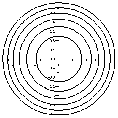
discussed in class, and is below.) To the right is a collection of
contours for f(x,y)=x2+y2. These contours
correspond to the positive integers 1, 2, 3, 4, 5, and 6.
Please notice how these contours, which are at evenly spaced
"heights", get closer together as the three-dimensional graph gets
steeper. Of course, if the contours are not labeled with the values of
the constants, I can't tell if the function is increasing or
decreasing! This picture was made with contourplot, another part of the
Maple package, plots.
|
|
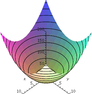 Here is one of the variations which can be produced with the plot3d command. It has the three-dimensional
(the two-dimensional picture of the three-dimensional graph!) plot
with the contour lines shwon at the correct places on the graph. There
are all sorts of views which can be obtained using the options of
plot and plot3d . Sometimes these variants can be
useful.
When this picture is rotated so we are looking down from the
positive z-axis, a view similar to the contour lines shown previously
is obtained.
|
The origin in this paraboloid graph is a local and absolute minimum. I
briefly sketched a graph of f(x,y)=–x2–y2, which
is an upside-down version of what was just drawn. So it has a local
and absolute minimum. That's not too new. But let's consider something
weird and wonderful.
A saddle
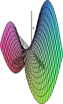
Consider the function f(x,y)=x2–y2 (I'm
trying to exaggerate the minus sign typographically in this since
that's the most interesting part). The traces are again "just"
parabolas. But here, when, say, y=2 (a plane transversal or
perpendicular to the y-axis), we get f(x,2)=x2–4. So the
curve z=x2–4 is a parabola opening up. As we change the y's
in this sort of slice, the bottom of the parabola moves down for big
|y|.
What about the other traces, with x=a constant? If x=3, then
f(3,y)=9–y2. In the plane perpendicular to the x-axis
given by the equation x=3, the curve is z=9–y2. a
parabola opening down. And by thinking we can see the top of these
parabolas moves up when |x| is large.
It may be difficult for a novice to see how to put these curves
together. To the right is a Maple graph
of this function for –3≤x≤3 and –3≤y≤3. When
you look at this on the computer (please try!) you can rotate it and
magnify it, and things might become more clear.
|
|
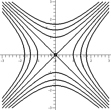
| The contour curves of this function are shown to the right.
Consider x2–y2=3, for example. One point on this
curve is x=2 and y=1, so look at the curve which goes through the
point (2,1). This curve is a hyperbola. The hyperbolas (each has two
pieces) corresponding to positive values of the function open left and
right. On the other hand, there is a family of hyperbolas opening up
and down. These correspond to negative values of the function.
And there's a special number. If x2–y2=0, then,
since x2–y2=(x+y)(x–y), the points on this
"curve" correspond to the two straight lines x=y and x=–y. (The
strange little box near (0,0) in the contour plot is because Maple thinks that very small +/– numbers which
it samples should also be 0. I am sorry about that. It may not be obvious looking at the curvy surface above that there are two straight lines on the surface. But there indeed are.
|
|
|
The point at the origin has a new kind of behavior, not found in one
variable calculus. In certain directions it is a maximum. In other
directions it is a minimum. This sort of point will be called a
saddle point (not too strange a name) or a minimax.
You could imagine that there will be a whole range of behaviors in
three hundred variables!
|
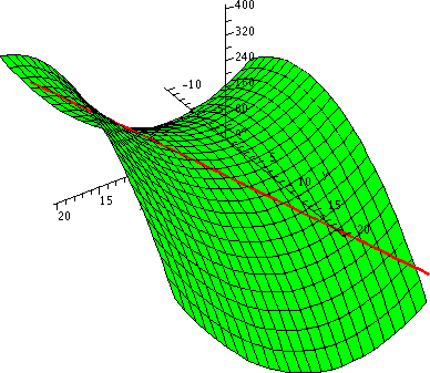
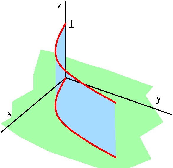
This saddle point is stranger than you might think. There are a heck of a lot of straight lines on this surface,
many more than you might think. For example, if x=7t+4 and y=–7t+5 and
z=112t–16 (these are parametric equations for some sort of
straight line!), then we actually get a value on the surface
z=x2–y2 for every value of t. This isn't
obvious. I could insert the formulas are check algebraically that
(7t+4)2–(–7t+5)2 is the same as 112t–16. Or I
could just show you a picture, to the right. After loading plots I typed
>A:=plot3d(x^2-y^2,x=-10..20,y=-10..20,axes=normal,color=green);
>B:=spacecurve(<7*t+3,-7*t+5,112*t-16>,t=-2..2,color=red,thickness=3);
>display3d({A,B});
and I got a version of the picture displayed to the right. On the
computer, you can rotate it and play with it, and sort of convince
yourself that the straight line actually is on the graph. Sort
of amazing.
Don't believe me! You try it.
|
| |
 Two half planes
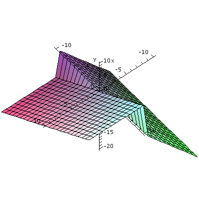
I defined a piecewise function to exercise "our" intuition.
        ( y  if x>0
f(x,y)= (
        (2x if x≤0
First, this function does depend on y. So we computed:
f(3,4)=4, f(–3,4)=–6, f(3,–4)=–4, f(–3,–4)=–6.
We discussed the graph of z=f(x,y).
The behavior on the two sides of the yz-plane (where x=0) is
different. More globally, the "rear" halfplane (where x<0) is a
half of a plane whose equation is z=y. This equation gives a plane
tilted at 45o to the y-axis. The front half, where x>0,
was a plane which was tilted up as y increased. The graph that is
shown is Maple's version. There are some real problems with
how the program shows this graph. The jumps, which we investigated
carefully, are connected because what Maple does is just connect
dots. So it connects the jumps even when these are not part of
the graph of the function (in 1 variable graphs, this "connecting"
idea can be turned off, but I don't know how to turn it off in several
variables). There are no vertical line segments in this graph!
I strongly recommend that you try to graph this function yourself, and
rotate the Maple plot systematically to understand what's going on.
How to define this function
Use the following, please:
>f:=(x,y)–>piecewise(x>0,y,2*x);
This command tells Maple that if x>0, then the value of f(x,y) is
y. If the statement is false, the value is 2x. Then I loaded the
package plots and just used the commands
plot3d and contourplot.
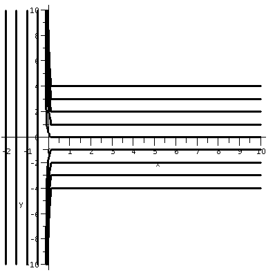 The contour "lines"
The contour lines are also not sketched too well. Most particularly,
the contour "line" f(x,y)=0 is very peculiar. It actually consists of
the y-axis together with the positive x-axis. Maple doesn't want to draw anything like that,
so it actually omits a line segment in this T-shaped contour line. I
tried various options with contourplot
but I could not get the T contour (C=0) drawn correctly. The other
contours are again for integer level sets. The level sets for C>0
are horizontal half lines in the first quadrant. The level sets fo
C<0 have two pieces. One part is a horizontal half line in the
fourth quadrant, and one part is a whole vertical line in the left
halfplane. This may be hard to visualize. I urged people to try to
educate their intuition. The left lines are closer together than the
horizontal halflines. This is all very very peculiar, but the worst is
to come.
|
The suicidal bug
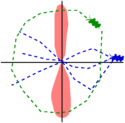 Now comes some of the harder stuff. I asked people to imagine that
some bugs were "walking" on the graph of z=f(x,y). The green bug, whose path is shown to the
right, strolls along in a path which is roughly circular around the
origin. This bug runs into trouble at any point on the positive
y-axis, where there's a drop. It also has problems along the negative
y-axis, where again there is a big difference in heights. This is a
very small bug. I have tried to indicate this by a sort of light
reddish color surrounding these half-lines. The
blue bug walks from the right halfplane to the left
halfplane. It is careful to cross only at the origin. The blue
bug is totally safe, and never comes across any severe height
differences. So I would like to discuss (and name [define], since it
is a math course!) the differences the bugs encounter more precisely.
Continuity
Almost all of the functions we will consider in this course will be
continuous (in fact, much nicer than just continuous -- they will be
smooth in a way that I'll explain later. But I should at least
remark on what continuity means. The definition should not be too
surprising.
A function f(x,y) is continuous at a point (a,b) in its
domain if lim(x,y)→(a,b)f(x,y) exists and is equal to
f(a,b).
Of course this doesn't help too much if we don't know what
lim(x,y)→(a,b)f(x,y) means. So I will discuss this very
briefly.
Limits in one dimension
In one variable, limits are relatively simple. To define
limx→af(x) we look at how x gets close to a from both
sides. There are some standard pictures and standard examples of
bad situations. Below are a few, to remind you.
| Bad limiting behavior in dimension
1 |
|---|
| A jump
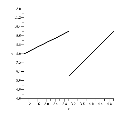
(y=x+7 for x<3, and 2x otherwise.)
|
Many wiggles
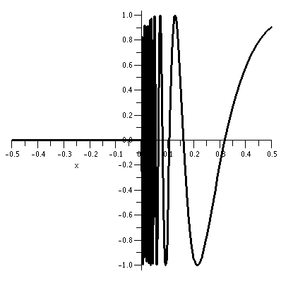
(y=sin(1/x) for x positive, y=0 otherwise.) |
|
Several variables
In several variables limiting behavior can be quite complex, much more
than with one variable. I tried to give a few examples.
Many straight line limits exist
I asked students to consider the function
f(x,y)=xy/(x2+y2)
This is an algebraic
formula which behaves is a strange fashion for (x,y) near (0,0). We
could try some values, but we can also take advantage of the
appearance of x2+y2. Almost always that's a
signal to at least attempt to understand things in polar coordinates
-- that is, to take advantage of circular symmetry.
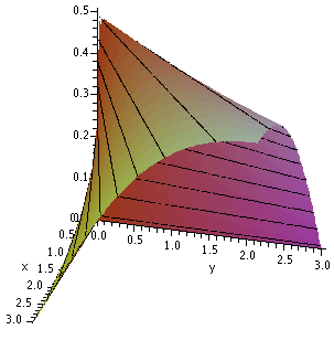
Since x=r cos(θ) and y=r sin(θ), we know that
x2+y2=r2 and
xy=r2cos(θ)sin(θ). Therefore
f(x,y)=xy/(x2+y2)=cos(θ)sin(θ)
The
value of f(x,y) only depends on the angular part of the polar
coordinate representation of (x,y) and not at all on the radial
component. The graph is made up of a bunch of half lines all parallel
to the xy-plane, radiating out from the z-axis. These halflines, since
cos(θ)sin(θ)=(1/2)sin(2θ), all have height between –1/2
and +1/2.
A Maple graph of the surface over the first quadrant (x>0
and y>0) is shown to the right. I also attempted, with the help of
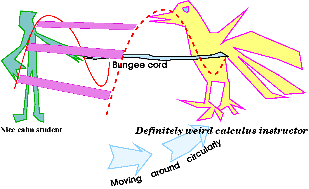
a stalwart student accomplice, to "draw" the surface kinetically. The
student "volunteer" held one end of a bungee cord under some tension
(both in the student and the cord!) while the calculus instructor held
the other end and walked around the student. The calculus instructor
raised and lowered the cord twice and the student was asked to keep
the end of the cord at the same level as the instructor's
end. Therefore along every angle a limit existed, but as the angle
changed, the limits changed. There were infinitely many
different limits possible along straight line approaches to
(0,0).
Always 0 on a straight line approach
 The final example of misbehavior was the following function:
 ( 1 if y=x2 and x>0
f(x,y)= (
( 0 otherwise
This function has only two values, 0 and 1. Certainly if you "walk"
towards 0 on a straight line approach in the second, third, and fourth
quadrants, the function values are all 0 and therefore the limit is
0. What's not so obvious perhaps is the behavior of the function on
straight line approaches in the first quadrant.
Look at y=x. This line intersections y=x2 only at x=0 and
x=1. So if we "walk" towards the origin on this line from some large
x>0 considering the values of the function f(x,y), the function
will be 0 at every point except x=1 where it will be 1. Certainly the
limit as x→0 will exist, and it will be 0.
In fact, the limit exists on every straight line approach to (0,0),
and the value of the limit is 0. But the real, two-variable limit
should not exist, because the values of f(x,y) do not get close to 0
as (x,y)→(0,0).
If you want more precise definitions of limits, here they are.
Limits, 1 dimension
Here we've got a function of one variable, and we want to define and
understand limx→af(x)=L. The actual definition,
frequently stated but rarely stressed in calc 1 classes, is the
following: (and, yes, the Greek letters ε and δ
are almost
always used)
|
Given any ε>0, there is some δ>0 so that if
0<|x–a|<δ, then |f(x)–L|<ε.
|
One way to possibly understand this is uses the model of a "function
box" as I did in class: a box labeled "f" which has input and
output. In this model, the ε is an output tolerance. We'd like
our outputs to be within ε of the ideal output (for this
problem) L. Then the limit definition states that there is some input
tolerance, δ, which when applied to stuff going into the machine
(only allowing inputs within δ of the initial input) then the
output tolerance will be satisfied. The definition itself may be
difficult to understand for several reasons. First, it is a
complicated logical statement, Second, it provides no structure for
computing or even estimating δ when actually given an
ε. To me, this is a bit distressing. But some understanding of
the input/output model and its approximation properties is fine right
now.
Limits, 2 dimensions
We looked at several examples which were not continuous and
did not have limits at (0,0). Let me show you the actual mathematical
definition of lim<x,y>→<a,b>f(x,y)=L. It is
very analogous to the 1 dimensional definition quoted above:
|
Given any ε>0, there is some δ>0 so that if
0<||<x,y>–<a,b>||<δ, then |f(x,y)–L|<ε.
|
Again the ε and δare output and input tolerances,
respectively. The interesting feature to me is
|<x,y>–<a,b>|. This means the distance from <x,y>
to the point <a,b>. This is distance in any direction, along any
path. The examples we saw last time only considered approaches to
<a,b> along straight line segments. This turns out not to be
enough. You've got to allow any paths, and, in fact, allow
consideration of all points close to <a,b> (a sort of blob
completely surrounding <a,b>). I think this makes limits much
more "strict" in several dimensions.
|
QotD
I introduced ∂ by just using
it. This was an interesting pedagogical exercise.
Example 1 If F(a,b,c)=a2b–3bc3 then
∂F/∂a=2ab and ∂F/∂b=a2–3c3 and
∂F/∂c=–9bc2.
Example 2 If F(a,b,c)=a3sin(7b–5c2) then
∂F/∂a=3a2sin(7b–5c2) and
∂F/∂b=a3cos(7b–5c2) and
∂F/∂c=a3cos(7b–5c2)(–10c).
The QotD was to compute
∂F/∂a, ∂F/∂b, and ∂F/∂c if
F(a,b,c)=a2e(7b–5c3).
So ∂F/∂a=2ae(7b–5c3),
∂F/∂b=a2e(7b–5c3)7, and
∂F/∂c=a2e(7b–5c3)(–15c2).
It turns out that
∂FUNCTION/∂VARIABLE,
when FUNCTION depends on many variables,
means that all variables except the variable specified are
thought of as constants, and then the derivative of the function with
respect to the remaining variable is computed with the help of the
usual algorithms.
Thursday, February 4, lecture #6
Here is a slightly different way to analyze 2-dimensional motion, and
this way will be more useful when we go to space curves (curves in 3
dimensions). I'll begin the class by rewriting the product rules
presented last time since I will need all of them today.
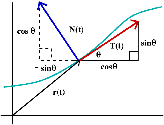 Let's define the unit tangent vector, T, to be a unit vector in
the direction of r´(t), the velocity vector. If θ is the
angle that r´(t) makes with the positive x-axis, then T must be
cos(θ)i+sin(θ)j. Also r´(t)=(ds/dt)T, where ds/dt,
the speed, is the length of r´(t). Now differentiate the formula
for r´(t) using one of the product rules we had stated earlier.
We get r´´(t)=(d2s/dt2)T+(ds/dt)dT/dt.
Let me show you one of the most interesting math/physical consequences of vector
calculus. Since T is always a unit vector, its length is 1
so T·T=1 (length squared!). Differentiate this equation and use
the product rule for dot products. The result is
dT/dt·T+T·dT/dt=0. But scalar product is commutative, so
the two terms are the same, and we can divide by 2 and get
T·dT/dt=0. That means dT/dt is perpendicular to T.
But T is cos(θ)i+sin(θ)j, and
dT/dt=(–sin(θ)(dθ/dt)i+(cos(θ)(dθ/dt)j=
(dθ/dt)[(–sin(θ)i+(cos(θ)j]. Now
dθ/dt=(dθ/ds)(ds/dt). But we called dθ/ds curvature,
κ, last time: the rate of change of the angle with respect to
arc length or with respect to speed reset to be uniformly 1. So
dT/dt=κ(ds/dt)[–sin(θ)i+(cos(θ)j]. The term
[–sin(θ)i+(cos(θ)j] is a unit vector perpendicular to T
and is usually called the unit normal vector and written N.
The equation
r´´(t)=(d2s/dt2)T+(ds/dt)dT/dt turns
into
r´´(t)= (d2s/dt2)T +
κ(ds/dt)2N.
We have decomposed acceleration into the normal and tangential
directions. This can be significant physically and can help to
understand physical and geometric situations. Here are two "extreme"
cases. Realize, as you consider them, that since F=ma and m, mass, is
a positive scalar, force is zero exactly when acceleration is zero and
also that force and acceleration have the same direction since
multiplication by a positive scalar doesn't change direction.
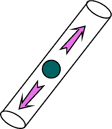
Motion in a straight line
Imagine a ball bearing (?) moving in a straight tube. I claim that the
tube never "feels" any force from the walls of the tube. Why? For a
straight line κ=0 always, the coefficient of the normal
component of the acceleration, κ(ds/dt)2, is always
0, for any motion, and therefore, since force is a scalar
multiple of acceleration, the force also must have zero normal
component. So the ball bearing can be pushed along or back in the
tube, but it is never pushed against the wall if you
insist that the ball bearing move in a straight path. There is
never any transverse force.
Motion in a circular arc
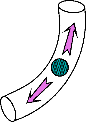 Now a more complicated thought experiment. Imagine the ball bearing
constrained to move in a piece of a circular tube. All we know is that
the object is moving, and its motion is part of a circular arc. I
claim that then, no matter what, the ball bearing is "feeling"
a transversal (normal) force from the "walls" of the tube. Why? The
normal component of the acceleration (a scalar multiple of the force
acting on the object) is κ(ds/dt)2. κ is not 0
since it is 1/(radius of the circle). And, since the object is moving,
we also know that ds/dt is not 0. Therefore the product isn't 0, and
the normal component of the acceleration isn't 0. There is
always a normal force.
This is, of course, related to the wonderful primitive experiment of
quickly spinning a bucket of water on a rope -- and the water is
"pushed" into the bucket by the "centrifugal force". Hey, that force
is a scalar multiple of the normal component of the acceleration of
the bucket's motion. It really works.
The geometry of space curves, curves in R3, as seen from
the point of view of calculus (called "differential geometry of space
curves") is a subject which originated in the 1800's. The material
presented here was stated in about 1850-1870. When I learned about
this material in college, it mostly seemed rather abstract and useless
-- stuffy formulas no intelligent person would care about. Like a
number of other judgments about merit that I've made in life, this is
completely wrong. The geometry of curves has within the last few
decades become very useful in a number of applications: robotics,
material science (structure of fibers), and biochemistry (the geometry
involving the structure of big molecules such as DNA), computer
graphics: amazingly useful formulas and ideas!
If r(t)=x(t)i+y(t)j+z(t)k (the position vector), then
r´(t)=x´(t)i+y´(t)j+z´(t)k=(ds/dt)T(t) is called
the velocity vector. Again, T(t) is called the unit tangent vector
and is a unit vector in the direction of r´(t). ds/dt is the
speed, and is
sqrt(x´(t)2+y´(t)2+z´(t)2),
the length of r´(t). We use ds/dt also to convert derivatives
with respect to t to derivatives with respect to s, as in two
dimensions using the Chain Rule.
Since T(t)·T(t)=1 differentiation
gives
T´(t)·T(t)+T(t)·T´(t)=0. But the dot product is
commutative, so this is 2T´(t)·T(t)=0 or just
T´(t)·T(t)=0.
This means that T´(t) and T(t) are always
perpendicular. In fact, we are interested in dT/ds, which is the same
as (1/(ds/dt))T´(t). It is usually easier to compute T´(t) directly,
however, and "compensate" by multiplying by the factor
1/(ds/dt).
Think about this sentence, which states something used repeatedly in
this course:
Any
non-zero(!) vector is the product of its magnitude multiplied by a
unit vector in its direction.
For dT/ds, the magnitude is
defined to be the curvature, κ, and the unit vector is
defined to be the unit normal N(t). This essentially coincides
with what's done for plane curves, when curvature was defined to be
dθ/ds.
Please remember the basic information about a
right circular helix. Click on the link and reread what we did if you
need to.
Here r(t)=a cos(t)i+a sin(t)j+btk, the position vector. The velocity
vector is r´(t)=–a sin(t)i+a cos(t)j+bk. The length of this
velocity vector is
sqrt([–a sin(t)]2+[a cos(t)]2+b2). This
simplifies because we know that
sin2+cos2=1. There are very few other
curvature computations which are so simple.
So ds/dt=sqrt(a2+b2) (the length of the velocity
vector, which is the speed) and we get the unit tangent vector by
dividing the components of r´(t) by ds/dt. So
T(t)=(1/sqrt(a2+b2))(–a sin(t)i+a cos(t)j
+bk). According to what we just did, if we differentiate this we
should get a vector perpendicular to T(t). Here we go:
d/dt(T(t))=(1/sqrt(a2+b2))(–a cos(t)i–a sin(t)j+0k). If
you take the dot product of this with T(t) you will get 0 (the
strange-looking signs make that true). But this is d/dt(T(t)) and, for
curvature, we need d/ds(T(t)). The Chain Rule suggests that I divide
d/dt(T(t)) by ds/dt to get d/ds(T(t)). If I do this, the result is
{1/(a2+b2)}(–a cos(t)i–a sin(t)j+0k). Wow. We
are not done yet. This should be κN: that is, it should be the
curvature, a positive number, multiplying a unit vector, and this is
the unit normal vector. If you stare at what we have you should
eventually see the following:
dT/ds={1/(a2+b2)}(–a cos(t)i–a sin(t)j+0k)=[a/(a2+b2)](–cos(t)i–sin(t)j)
Here what is in blue is a scalar, multiplying
what is in green which is a unit
vector. Therefore what is in blue is κ,
the curvature, and what is in green is the
unit normal vector. By the way, this is why everyone (and me too, darn
it, me too!) uses formulas such as those in the book to compute these
things, because direct computation from the definition is too
complicated.
If κ=[a/(a2+b2)] for the
helix, how does this match up with our forecasts? Here is the scorecard.
- If a→∞, then κ→0+. The curve gets
flatter.
When a gets large, we have a1 on top and essentially
a2 on the bottom. The result certainly does →0.
- If b→∞, then κ→0+. The slinky (?)
gets stretched out more.
Here if a is fixed, and b gets really large, again the result ;→0
because b only appears on the bottom.
- If a=0, then κ=0. The curve is a straight line.
True -- set a=0 in the formula.
- If b=0, then κ=1/a. The curve is a circle.
Again, if b=0 in the formula, then the result is a/a2
and this is 1/a.
Very few other computations of curvature are this simple.
Here are some pictures of various helices produced by Maple (the plural of "helix" is
"helices").
The pictures below were produced using the command
spacecurve([a*cos(t),a*sin(t),b*t],t=0..6*Pi,axes=normal,color=black,thickness=2,scaling=constrained,numpoints=180);
The procedure spacecurve is loaded as
part of the plots package using the
command with(plots);. I used the option
scaling=constrained in order to "force"
Maple to display the three curves with
similar spacing on the axes. Otherwise the x and y variables would be
much altered in each image. I hope that these pictures help you
understand what curvature represents.
| Some helices: x=a cos(t);
y=a sin(t): z=bt.
|
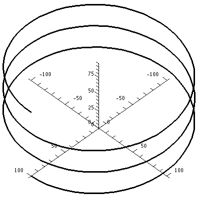 | 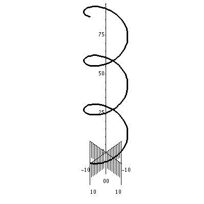 | 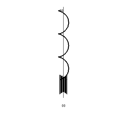 |
a=100 & b=5
κ=.01 |
a=10 & b=10
κ=.05 |
a=5 & b=100
κ=.0005 |
|
The curvature of the twisted cubic
O.k., I tried to compute the curvature of
r(t)=ti+t2j+t3k. I used a formula from section 13.4:
κ=||r´(t)xr´´(t)||/(||r´(t)||)3.
Even though this formula looks weird, it is much better to use than
trying to work through the definitions. I have tried using the
definitions with this example, and the computations are terrible.
So r´(t)=1i+2tj+3t2k and
r´´(t)=0i+2j+6tk. Now for the cross product computation:
   | i  j  k |
det| 1 2t 3t2| = det|2t 3t2| i– det|1 3t2| j + det|1 2t|k
   | 0  2 6t |      | 2 6t |       |0 6t |        |0  2|
And then I evaluated the 2-by-2 determinants, so we saw that the
vector on the top of the formula for κ is
(12t2–6t2)i–6tj+2k=(6t2)i–6tj+2k. But
we need the magnitude or length of this for the top, and this is
sqrt(36t4+36t2+4). Wow. The bottom is the
three-halves (!) power of the length of the velocity vector, and this
is (1+3t2+9t4)3/2.
Therefore (as they write in textbooks) the curvature of the twisted
cubic is
sqrt(36t4+36t2+4)
----------------------------
(1+3t2+9t4)3/2
Now, after this {ludicrous|wonderful} computation, I do admit that I get
almost nothing out of it. Here is this ridiculous formula, and what
does it tell me? Maybe a little bit: If t is very large positive
or very large negative, it seems to say that the curvature gets small
(look at the "net" power of t on top, maybe a t2, and on
the bottom "net" a sort of t6). I guess this means that the
curve gets flatter as |t|→∞. Maybe this is interesting. (It
sort of resembles y=x2 that way.)
How to think of all this?
What would I like "you" (especially the engineer and physics "yous")
to take away? Another formula from the textbook (section 13.5) resembles exactly what we already saw in two dimensions:
r´´(t)= (d2s/dt2)T +
κ(ds/dt)2N
This is a decomposition of the acceleration vector into
tangential and normal components, and it does have some interesting
information about physical quantities as we saw in two dimensions for
the straight line and the circle.
A little bit more ...
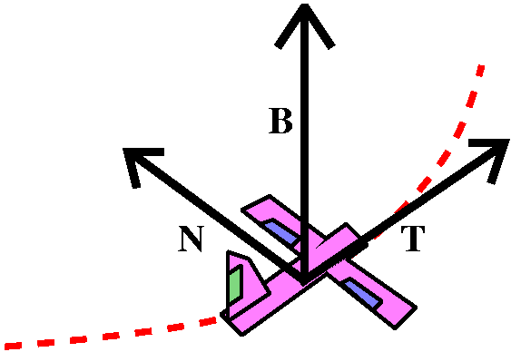 I hate to leave this subject since there is much more to be told, and
everything turns out to be amazingly useful in a wide variety of
applications. I hate to leave the subject, but the course is very
dense. So: a little bit more. Think of an airplane flying along a
curve in the sky (the dashed red line). Then the unit tangent and
normal vectors are as shown. There's another vector, B, called the
binormal vector, which is TxN. Since T and N both have
length 1 and they are perpendicular, then B also has length 1 (sine of
a right angle is 1). And B is perpendicular to both T and N.
The right-handed triple T, N, B is called the Frenet
frame. Describing how this "frame" changes in time tells a lot
about the curve. The curvature says how much the airplane is being
pulled from a straight line. It measures how much the T is changing in
the N direction. The green surface on the
tail or the rudder of the plane is the major object determining
κ. But the motion is three-dimensional. The way the binormal, B,
changes, says how much the airplane is twisted out of the
two-dimensional plane determined by T and N. The rate of change of B
is called the torsion, and is determined mostly by the angles
that the blue control surfaces have with the
wings. When a plane takes off or is landing, these surfaces have
relatively high angle to the wings. Let me do things with a bit more
detail.
I apologize to any pilots, because
what's above is not exactly correct. Actually, they would be thinking,
"That's not correct at all". I am certainly simplifying.
Reality is more complicated.
Also, right now I'm losing the advantage I got on the first day
compared to the standard syllabus because I'm using an extra lecture
for this material. Oh well.
How does B(t) change? Since B(t)·B(t)=1, differentiation results in
2B´(t)·B(t)=0, so B´(t) is orthogonal to B(t). But differentiation of
B(t)=T(t)xN(T) results in B´(t)=T´(t)xN(t)+T(t)xN´(t). Since T´(t)
is parallel to N(t) (because of our definition of N(t)!), the first
product is 0 (another property of cross-product!) so that B´(t) is a
cross-product of T(t) with something. Therefore B´(t) is also
perpendicular to T(t). So B´(t) is perpendicular to both T(t) and
B(t), and since only one direction is left, B´(t) must be a
scalar multiple of N(t). The final important definition here for space
curves is: dB/ds is a product of a scalar and N(t). The scalar is
–τ. That is supposed to be the Greek letter tau, and the
minus sign is put there so that examples (the most important is coming
up!) will work out better. This quantity is called torsion, and
is a measure of "twisting", how much a curve twists out of a plane
(the particular plane is the plane determined by T and N).
If a space curve does lie in a plane, and if everything is nice and
continuous, then B will always point in one direction (there are only
two choices for B, "up" and "down" relative to the plane, and by
continuity only one will be used) so that the torsion is 0 since B
doesn't change. The converse implication (not verified here!) is also
true: if torsion is always 0, then the curve must lie in a
plane!
Let me apply this to the right circular helix with a direct
computation. I emphasize that this is by far the simplest example, and
almost all curvature and torsion computations I've done in the last
decade or so have used computer algebra systems.
So for our helix with r we
found
T(t)=1/sqrt(a2+b2))(–a sin(t)i+a cos(t)j+bk);
N(t)=–cos(t)i–sin(t)j;
ds/dt=sqrt(a2+b2).
So B(t)=T(t)×N(t). This is the scalar
1/sqrt(a2+b2)) multiplying
the cross product of
–a sin(t)i+a cos(t)j+bk and
–cos(t)i–sin(t)j: | i j k |
det |–a sin(t) a cos(t) b | = b sin(t)i –(–b)(–cos(t))j+a(sin2+cos2)k
| –cos(t) –sin(t) 0 |
Yes, there really are 3 minus signs and a trig identity. So
B(t) is the vector
(1/sqrt(a2+b2))(b sin(t)i–b cos(t)j+ak).
A few questions:
- Is B(t) a unit vector? Its length is
(1/sqrt(a2+b2))sqrt(b2sin(t)2+b2cos(t)2+a2)
which is
(1/sqrt(a2+b2))sqrt(a2+b2)=1.
- Is B(t)⊥T(t)? The dot product of
(1/sqrt(a2+b2))(b sin(t)i–b cos(t)j+ak)
and
1/sqrt(a2+b2))(–a sin(t)i+a cos(t)j+bk)
is ab–ab=0.
- Is B(t)⊥N(t)? The dot product of
(1/sqrt(a2+b2))(b sin(t)i–b cos(t)j+ak)
and N(t)=–cos(t)i–sin(t)j. is
(–b)–(–b)=0.
Now for the torsion we need to find dB/ds. I compute dB/dt and get
(1/sqrt(a2+b2))(b cos(t)i+b sin(t)j).
To get dB/ds we multiply by 1/(ds/dt) which is
1/sqrt(a2+b2). The result is
(1/(a2+b2))(b cos(t)i+b sin(t)j).
This is supposed to be –τN(t) where
N(t)=–cos(t)i–sin(t)j.
Now notice that the darn minus signs cancel (that's one of the reasons
for the minus in the definition of τ) and we see clearly
that for a right circular helix,
τ=b/(a2+b2). If b=0 this is a circle in the
plane, and the torsion is 0. Intuition about torsion is hard to get.
Curvature tells how T changes, and torsion tells how B changes. What
about N? In fact, if we look at the expression N=BxT and differentiate, using the product rules
again, no new quantities are needed (this is done in detail
below). The result is called
the Frenet-Serret equations (also called
the Darboux equations in mechanics):
dT/ds =  0 + κN +  0
dN/ds =–κT +  0 + τB
dB/ds =  0  –τN +  0
These are three vector differential equations, so they actually
represent nine (9) scalar differential equations and there is
considerable significance in the way these equations look. If you
want to move robot arms or analyze molecular backbones, then ... you
may need to deal with these equations.
The first and third equations are used to define κ and
τ. Their information content is that the rate of change of both T
and B is in the direction of N which is maybe a bit surprising. The
middle equation is the one that, to me, is really startling: the rate
of change of N can be predicted from the quantities already defined --
nothing new needs to be considered.
Getting the middle equation
Since N=BxT, we can differentiate with the
appropriate product rule, using the other two equations. If we d/ds,
then dN/ds=dB/dsxT+BxdT/ds=–τNxT+BxκN. Remember that T,N,B is a right-handed
coordinate system. Therefore TxN=B so that
NxT=–B. And NxB=T so that BxN=–T.
Therefore dN/ds=–τNxT+BxκN=τB–τT. This is the middle
equation in the collection above.
|
Stay calm!
Consideration of torsion is not officially part of the course,
and neither are the Frenet-Serret (Darboux) equations. And also no
binormals. So stop worrying. There is more about all this in the
textbook if you are interested. And also in books about motion,
molecules, materials, ...
 QotD
QotD
Here is a formula for torsion from Wikipedia.
I think it is correct. The first version of the formula that I wrote
(with the exponent=2 in the bottom!) was correct, darn it! I suggested
3 which was incorrect and I
am very sorry. I will "correct" the answers taking this into accout.
The management, looking sorry, is shown to the right.
If r´, r´´, and r´´´ are the first three
derivatives of the position vector (velocity, acceleration, and what
is sometimes called jerk), then
    (r´×r´´)·r´´´
τ= ---------------
     ||r´×r´´||2
Suppose r´(0)=<2,1,0>, r´´(0)=<0,–2,1>, and
r´´´(0)=<–1,0,1>.
Compute the torsion, τ, of the curve at time 0.
Answer r´×r´´ turns out to be
<1,–2,–4> and then τ=–5/21.
Monday, February 1, lecture #5
Various differentiation formulas
I should have written these last time. Here are some general formulas
for differentiating vector-valued functions as they interact through
vector algebra.
Here we suppose that
v1(t)=<x1(t),y1(t),z1(t)>
and
v2(t)=<x2(t),y2(t),z2(t)>
are both differentiable (this is logically the same as asking that all
6 of the scalar functions x1(t), ... ,z2(t) be
differentiable.)
- Differentiation and vector addition
If w(t)=v1(t)+v2(t), then w(t) is a
differentiable vector-valued function, and
w´(t)=v1´(t)+v2´(t).
- Differentiation and dot product
If f(t)=v1(t)·v2(t), then f(t) is
a differentiable scalar-valued function, and
f´(t)=v1´(t)·v2(t)+v1(t)·v2´(t).
- Differentiation and cross product
If w(t)=v1(t)×v2(t), then w(t) is
a differentiable vector-valued function, and
w´(t)=v1´(t)×v2(t)+v1(t)×v2´(t).
- Differentiation and scalar multiplication
Suppose c(t) is a scalar-valued differentiable function. Then
w(t)=c(t)v1(t) is a vector-valued differentiable function,
and w´(t)=c´(t)v1(t)+c(t)v1´(t).
These formulas can be verified by writing out the components and using
calc 1 techniques. For example, the dot product
v1(t)·v2(t) is, in more detail,
x1(t)x2(t)+y1(t)y2(t)+z1(t)z2(t),
a collection of standard real-number products connected by sums. If we
differentiate, the result using the standard product formula (I'll
just write the result of differentiating the first term) is
x1´(t)x2(t)+x1(t)x2´(t).
I hope you see that this is the first part of each of the pieces
in the sum which was given:
v1´(t)·v2(t)+v1(t)·v2´(t).
Use the cross-product formula with some care since cross-product is
not commutative. The order in the terms matters.
What will we do?
Today I want to use calculus as a way of investigating the geometric
properties of curves. This is a bit difficult because calculus applies
to the parameterizations of the curves, and since there can be many
sometimes wildly different parameterizations of the same curve, we'll
need to be clever. This material was mostly developed between 1750 and
1850. It has been found useful recently in such subjects as molecular
biology (describing how long molecules might twist) and computer
graphics (what curves should shadow and light make?).
Arc length
If speed is the magnitude of the velocity vector, then since
distance=rate·time, then, with variable speed, we need to chop
up the time interval and compute and add up pieces of distance. This
is the basic idea behind the definite integral, so it makes sense to
compute the distance along a curve from time t1 to time
t2 by this:
∫t1t2||v(t)|| dt.
O.k., this is good (all math is good!) but maybe some
examples ... will show how silly it is.
Textbook example
Here is an example taken from a textbook. Suppose
r(t)=<12t,8t3/2,3t2>. What is the length
of the curve from t=0 to t=1?
This is a typical artificial problem in a textbook. We know that
r´(t)=<12,8(3/2)t1/2,6t> so that the
speed is
||r´(t)||=sqrt{122+122t+36t2}. Now
we "remember" that distance=rate·time, and that the magnitude
of the velocity vector is ds/dt, the speed. So the total distance
traveled is
∫01sqrt{144+144t+36t2} dt.
Now look at the coincidences. We can pull out the 36 from under the
square root, and the result is
6∫01sqrt{4+4t+t2} dt, and,
what a coincidence, 4+4t+t2 is (2+t)2 and the
integral becomes 6∫01(2+t) dt=6(2t+(1/2)t2]01
and this is 6[2+(1/2)].
More realistically ...
Almost every combination of two or three functions, even rather
"simple" functions that you try to use as a position vector, will
yield something that can't be antidifferentiated in terms of familiar
functions. For example, look at the following mess:
> a:=t->t^3;
                                            3
                                 a := t -> t

> b:=t->cos(t);
                               b := t -> cos(t)

> c:=t->exp(t);
                               c := t -> exp(t)

> int(sqrt(a(t)^2+b(t)^2+c(t)^2),t=0..1);
bytes used=4000036, alloc=3407248, time=0.14
bytes used=8007244, alloc=5241920, time=0.30
                         1
                        /
                       |     6         2         2 1/2
                       |   (t  + cos(t)  + exp(t) )    dt
                       |
                      /
                        0
And that means Maple tried but can't
figure out anything useful to reply except to echo the integral back
to the questioner. My next step is> evalf(%);
1.971185471 which asks for
an approximate (numerical) evaluation of the integral. That's almost
always what's going to be necessary. Oh well: the situation in
textbook problems is much too nice.
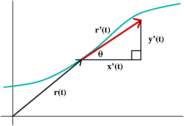 Curvature is a number which measures how a curve bends
I tried to analyze the idea of how a curve bends. Curvature will be a
measure of this bending. What I'll show you is an analysis that was
apparently first done by Euler in about 1750. First we'll consider
plane (2-dimensional) curves. A curve is a parametric curve, where a
point's position at "time" t is given by a pair of functions,
(x(t),y(t)). Equivalently, we study a position vector,
r(t)=x(t)i+y(t)j. Here x(t) and y(t) will be functions which I will
feel free to differentiate as much as I want.
There are some special test cases which I will want to keep in mind.
#1: a straight line
A straight line does NOT bend, so it should have curvature 0.
#2: a circle
A circle should have constant curvature, since
each little piece of a circle of radius R>0 is congruent to each
other little piece, and, in fact, the curvature should get large when
R gets small (R is positive), and should get small when R gets large
(and looks more like a line locally).
#3: "the" parabola
Even y=x2 might be a good test to keep in mind, since there
the curvature should be an even (symmetric with respect to the y-axis)
function of x, and should be bell-shaped, with max at 0 and limits 0
as x goes to ±–∞. The curve actually bends most near the
origin, and far away, when x is large positive or large negative, even
though the curve is very steep, it gets really flat.
The problem of understanding or defining curvature is to somehow
extract the geometric information from the parameterized curve. That
is, if a particle moves faster, say, along a curve, it might seem like
the same curve bends more. So what can we do? Somehow the
geometry of the curve should be separated from the dynamics
(kinetics?) of motion along the curve.
We looked at
θ, the angle that the velocity vector r´(t) makes with respect to
the x-axis. How does θ change? After some discussion it was
suggested that we look at the rate of change with respect to arclength
along the curve: that is the same as asking for the rate of change
with respect to travel along the curve at unit speed, and therefore
somehow the kinetic information will not intrude on the
geometry. This is the same as asking a bug to travel along the curve
at unit speed, and to describe the rate of change of θ (the
turning of r´(t), the velocity vector) as the bug strolls along
the curve.
The quantity s and the quantity t
Arc length, s, on a curve is computable with a definite integral:
sqrt(x´2+y´2) integrated from
t0 to t with dt is the arc length. As shown before, this is
rarely exactly computable with antidifferentiation using the usual
family of functions. But ds/dt is just
sqrt(x´2+y´2) by the Fundamental
Theorem of Calculus. And the Chain Rule suggests that (dFROG/ds)(ds/dt)=dFROG/dt if FROG is any quantity
of interest, such as θ. So to get dFROG/ds from dFROG/dt, multiply the
latter by 1/(ds/dt) which is
1/sqrt(x´2+y´2).
By drawing a triangle we see that θ is arctan of y´/x´:
θ=arctan(y´/x´). We can find dθ/dt: it is
(y´´x´–x´´y´)/(x´2+y2)2. This uses
the formula for the derivative of arctan, the Chain Rule, and the
quotient rule. Then the previous results say that
dθ/ds=(y´´x´–x´´y´)/(x´2+y´2)3/2,
a complicated formula. This is what's called curvature,
κ (this Greek letter kappa is usually used for curvature).
Back to the test cases
The straight line
We compute for some constants A and B and C and D:x(t)=At+B x´(t)=A x´´(t)=0
y(t)=Ct+D y´(t)=C y´´(t)=0
so that the top of the curvature formula is 0.
κ=0 for any straight line. |
|
A circle
Suppose we have a circle of radius R centered at the origin.
Then parametric equations are not too difficult to get:x(t)=Rcos(t) x´(t)=–Rsin(t) x´´(t)=–Rcos(t)
y(t)=Rsin(t) y´(t)=Rcos(t) y´´(t)=–Rsin(t)
Let me look first at the bottom of the curvature formula. This is
(x´2+y´2)3/2. Notice that
x´2+y´2=R2([–sin(t)]2+[cos(t)]2)=R2,
so the 3/2´s power is R3. The top is
y´´x´–x´´y´ and this is
–Rcos(t)(–Rsin(t))––Rcos(t)Rcos(t)=R2·1. The whole
curvature formula is then R2/R3 which is 1/R.
When R is large, this is near 0. When R is close to 0 and positive,
this is large positive. And the curvature is constant which it should
be since the circle has the same local geometry at every point.
|
|
A parabola
Here I want to look at y=x2. A simple parameterization
is good. So let's try:x(t)=t x´(t)=1 x´´(t)=0
y(t)=t2 y´(t)=2t y´´(t)=2
Now the bottom of κ,
(x´2+y´2)3/2,
becomes (1+4t2)3/2, and the top,
y´´x´–x´´y´, is just 2. So
κ=2/(1+4t2)3/2.
Here the "local geometry" definitely changes from point-to-point. The
most curvy (?) part of the graph is at the origin. As x→±∞,
although the graph gets steeper and steeper, the curve locally
actually gets more and more flat: the curvature→0.
|
The smaller figure is supposed to be the curvature of the parabla.
|
The right circular helix
This will be our 3-dimensional "test case".
We'll consider a right circular helix.
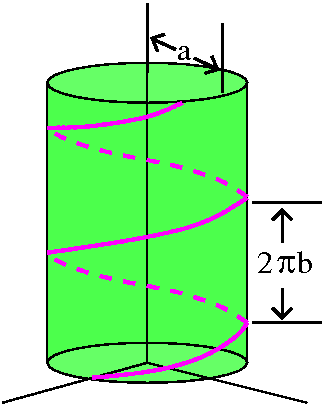
x(t)=a cos(t)
y(t)=a sin(t)
z(t)=b t
The quantities a and b are supposed to be positive real numbers.
This helix has the z-axis as axis of symmetry. It lies "above" the
circle with radius a and center (0,0) in the (x,y)-plane. The distance
between two loops of the helix is 2π b. The "b" changes the
pitch or angle of the screw threads modeled by the helix.
How should curvature behave for the helix? We discussed this and
decided κ should have these properties:
- If a→∞, then κ→0+. The curve gets
flatter.
- If b→∞, then κ→0+. The slinky (?)
gets stretched out more.
- If a=0, then κ=0. The curve is a straight line.
- If b=0, then κ=1/a. The curve is a circle.
QotD
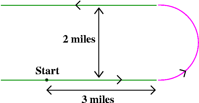 A racetrack: this racetrack consists, as nearly as possible, of two
straight line segments, each about 3 miles long, connected with a
semicircular track. Since the racetracks were specified to be 2 miles
apart, we "deduce" that the radius of the semicircle is 1 mile. The
racetracks certainly have curvature=0, and the semicircle, which is
Π units long, has curvature 1. What would a graph of the curvature
of this racetrack look like? (This is supposed to something
real and I'd like motion along this racetrack to be smooth, so
the curvature graph should at least be continuous!)
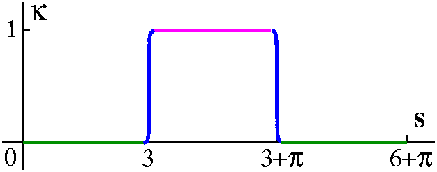 An answer
I attempted to be "correct" both qualitatively and quantitatively in
this graph. The blue curves are
my attempts to draw smooth transitions between the curvatures of the
circles.
Thursday, January 28, lecture #4
| If you did not attend the recitations on Tuesday, January 26,
we (Mr. Nanda and I) strongly recommend that you follow the
links on this
web page, and print out the General Introduction and the four "Playing
with ..." files. Then go to a Rutgers computer lab and work through
the "Playing with ..." pages. It is probably easier and certainly more
fun if you can do this with another person working at the same task on
a nearby computer. Maple will be
needed in several assignments in this course and it may help you
explore and learn some of the course material.
|
editorial editorial editorial editorial editorial editorial
Comments on the economics of colleges
and the specifics of Math
251
California ... capacity ... attendance ... homework
editorial editorial editorial editorial editorial editorial
Vector functions of a real number
Now the course moves on: we will deal with functions whose domain is
all or part of R1 and whose range is R3. These
are vector-valued functions of a scalar variable. The motivation is
really the motion of points in space, and the analysis of the
resulting paths (curves). There will be interactions between motion
and geometry.
Parametric curves: a nuisance?
So I began with some irritating examples.
- The curve
r(t)=<t,t,t>. This curve is a straight line. It goes through the
origin, (0,0,0), and the path described is all of the line. The motion
described by this vector function (a triple of standard real-valued
functions) is uniform rectilinear (straight-line) motion.
- The curve r(t)=<t3,t3,t3>
is all of the straight line, but the kinetic aspect is very
different. Motion is not uniform, and gets faster as |t| gets larger
both positive and negative.
- Now the curve
r(t)=<t2,t2,t2> is not too
surprising. It is a half line or ray. Dynamically this represents the
motion of a point starting way out in the first octant where all of x
and y and z are positive, then coming in (slower and slower) to
(0,0,0). Then the point turns around (?) and starts out into the
octant again, retracing its path and going faster and faster.
- The curve r(t)=<sin(t),sin(t),sin(t)> is quite nasty
psychologically if discussed immediately after the line. All of the
coordinates are equal so every point on this curve is on the straight
line. Some thought is needed to force yourself to agree that the
"curve" is only a line segment from (–1,–1,–1) to (1,1,1) because
sine's range is [–1,1]. The motion described by this vector function
oscillates endlessly between the two points named.
Distinguishing between geometric aspects of the path of a particle and
the dynamic aspects of the particle will take up most of our next
class. This won't be obvious.
Two problems in the textbook
I tried to discuss two problems from the textbook. These pictures are
copied from page 743 of the text.
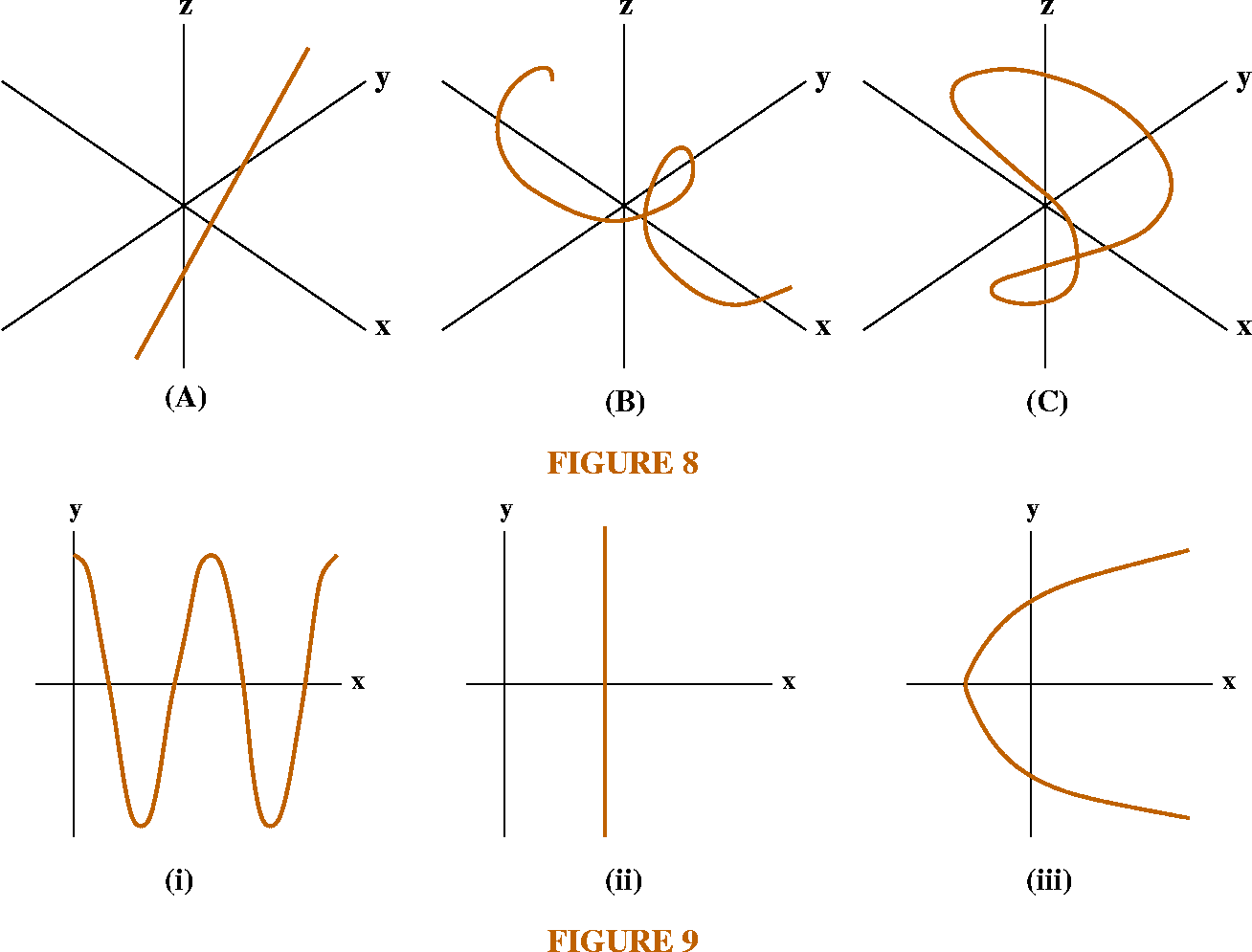
Problem 5 of section 13.1
Match the space curves in Figure 8 with
their projections onto the xy-plane in Figure 9.
Answer
How can we "solve" this problem? I actually think
most people can solve the problem, but I think describing the process
is somewhat difficult. It is difficult because, for example, the
pictures in Figure 8 are two-dimensional. And they are images of some
ideal three-dimensional situation. What can we see? In Figure 8 (A) I
see a straight line. I believe that the straight line will not be made
"curvy" if we project into the xy-plane. Therefore the only candidate
which matches is the non-curvy (!) picture (ii) in Figure 9. What
else? Maybe the picture in (B) seems to be helical (more precise
information about a helix later). That's sort of a motion around a
cylinder whose axis of symmetry is, in this case, the x-axis. If we
push this down and neglect the z coordinate, I think what we get is
picture (i). This leaves (C) matching up with (iii). If you think
about a particle moving around the path indicated in (C), maybe
you see the xy-"squashing" of it moving back and forth along the
parabolic path in (iii). Is this somehow "proof" that this was (iii)?
We're told that the triples of pictures match up, and (C) and (iii)
are what's left. It is certainly true that something like (C) could
have a more complicated squashing than what is in (iii).
Problem 6 of section 13.1
Match the space curves in Figure 8 with the following vector-valued
functions:
(a) r1=<cos(2t),cos(t),sin(t)>
(b) r2=<t,cos(2t),sin(2t)>
(c) r3=<1,t,t>
Answer
Well, the linear formula is (c), and if we just
consider the first two coordinates, the 1 and the t, that would seem
to describe (ii), so I think that (c) is the algebraic version of
(A). As for (b), the first two coordinates are t and cos(2t) which
seem to describe (i). And if you consider the second and third
coordinates of (b), they are cos(2t) and sin(2t). The sum of the
squares of these is 1 (cos2+sin2=1) and the
first coordinate in (b) just moves the point along, so we get the
helix in (B). That leaves r1 in (a) to describe (C) and
(iii). Let's consider the first two coordinates of (a), which are
cos(2t) and cos(t). A trig identity you may/may not remember is
cos(2t)=2(cos(t))2–1. If we take x as cos(2t) and y as
cos(t), this becomes the equation x=2y2–1 which surely
looks like (iii). And the third coordinate, sin(t), of (a) makes the
image go up and down, up and down. So (a) is consistent with both (C)
and (iii). I think this third curve and formula are a bit interesting
and strange.
Pictures of a point in motion
Twisted cubic
The twisted cubic is the curve
r(t)=<t,t2,t3>. It is one of the beginning
curves shown to students in this subject, with the warning that here
is the pictures can be deceptive. A Maple command created a
3-dimensional viewing box of the curve. I rotated this box in various
ways and exported the images shown below.
spacecurve(<t,t^2,t^3>,t=–5..5,color=black,axes=normal,thickness=2);
| The view from the z-axis
Here we look down on the curve from high up on the z-axis. This has
the effect of suppressing (?) or deleting the z-coordinate from the
triple, and we just see the geometry of the first two coordinates:
(t,t2). Of course, this is the parabola y=x2.
|
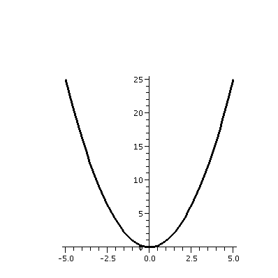
|
| The view from the y-axis
Now delete the central variable. In the xz-plane, the curve is the
collection of points (t,t3) and this is z=x3,
which is, I hope, a fairly familiar cubic. And, indeed, if you orient
the twisted cubic properly, then Maple shows you the
displayed picture.
|
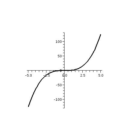
|
| The view from the x-axis
This is picture which makes life difficult. Projected only the
yz-plane, the collection of points (t2,t3) is
the same as those points satisfying y3=z2. Now
since z2 must be non-negative, any y's on this curve had
better be in the right half of the yz-plane. And for each y>0,
there are two z's (the positive and negative square roots). But the
worst part is the behavior at the origin. z=+/–y3/2 has a
horizontal tangent at (0,0): the curve has what's known as a cusp at
the origin, a type of corner. It looks sharp, not smooth! This
non-smooth behavior is officially called a cusp.
|
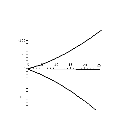
|
An oblique view
This "curve" actually does not have a corner in
three-dimensions. The pictures already shown do not make this easy to
see. To the right is sort of an oblique view of the curve as drawn by
Maple. Although this picture seems to
show a loop, the curve does not actually have any loops. The loopy
look is a result of the angle I picked. The difficulties I discussed
here are one reason the instructors would like you to be familiar with
Maple -- use of it will help your
intuition.
A perspective on real life
Frequently, similar difficulties have occurred in dissections of
bodies, when slides of different cells are prepared. Depending on the
angles of the slices, very different pictures are seen.
|
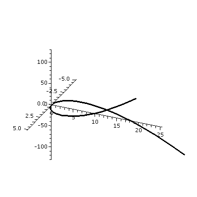
|
Robots and molecules
People who want to understand the conformation (geometry) of
biologically interesting macromolecules will need to learn how to look
at curves in R3. Also, people who want to describe motion
of robot arms necessarily need the ideas we will describe.
The derivative
If r(t)=<a(t),b(t),c(t)> is a vector function of t, we can
consider (1/h){r(t+h)–r(t)}. Inside the {} is a difference of vectors,
and that's therefore a vector. Then multiplying by 1/h: that's a
scalar multiple. So the result is a vector. It may happen that the
limit as h→0 of this quotient may or may not exist. If it does,
we'll say that r(t) is differentiable and that the limit, which is
labeled r´(t), will be called the derivative. It is also called the
velocity vector.
It doesn't take many examples to convince yourself that the (vector)
derivative will exist exactly when all of the scalar functions a(t)
and b(t) and c(t) are differentiable, and that the components of the
resulting vector derivative will be the derivatives of these
functions. That is, if a(t) and b(t) and c(t) are differentiable, then
the vector function will also be differentiable, and
r´(t)=<a´(t),b´(t),c´(t)>. Computing the
derivative of such a vector function when the component functions are
defined by familiar formulas involves nothing essentially new. I did a
few examples.
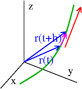 Meaning of the derivative
The derivative balances out a large scalar, 1/h (when h is small),
with a very small secant vector, r(t+h)–r(t). To the
right is shown a possible picture of the situation. The the secant vector, r(t+h)–r(t) is in
magenta. It is close to the curve, with its
head and tail at two nearby points on the curve. That the limit
exists is rather neat fact, that somehow the shrinking of the vector
stabilizes with the increasing of the scalar amount, and that the
direction tends to a fixed direction -- this is not obvious, and one
should really not expect it! This direction is a vector, drawn in red. It is called the velocity vector
or the tangent vector.
The magnitude: speed
The magnitude of the velocity vector, ||r´(t)||, is called the
speed.
Velocity vector, tangent vector
I tried to argue, looking at a local picture of the path of a
particle, that the direction of the velocity vector is tangent to the
path of the particle. So the velocity vector is a vector
tangent to the path.
So I had considered parameterizations of various portions of a
straight line earlier in this lecture. Let's look at the speed of the
parameterizations.
<t,t,t> has derivative <1,1,1> with speed therefore sqrt(3): a
constant. So this is a uniform speed parameterization.
<t3,t3,t3> has derivative
<3t2,3t2,3t2> with speed
therefore sqrt(3)3t2. For t large negative or positive, the
speed is large. It decreases near 0 and the speed is 0 at
0. This is what we observed when considering the graph. Also the
direction is always (except t=0!) <positive,positive,positive,>.
Now consider <t2,t2,t2>.
The velocity vector is <2t,2t,2t>. For t<0 it points towards
the origin, and for t>0 it points away from the origin, as we saw
earlier. And the speed is sqrt(3)2|t| (remember that the square root
of t2 is |t|, not t!). So this is large when |t| is large.
And finally <sin(t),sin(t),sin(t)> has speed sqrt(3)|cos(t)|,
which varies periodically also as predicted.
|
Tangent line to a helix
Look at the curve r(t)=<3cos(2t),3sin(2t),8t>. What is this?
The first two variables describe uniform circular motion. The radius
of the circle is 3, and that's the distance from the central axis of
this curve, which turns out to be a helix. The 2 changes the angular
velocity of the curve, and doubles it. 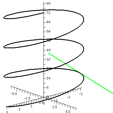 The 8 affects the "pitch", the
angle of the helix, and also the distance between "loops". When 2t
changes by 2Π, the curve passes around one loop. That means the
change in t is Π, so the change in z is 8Π.
Let's find the parametric equations of a line tangent to this helix
when t=Π/2. The line must pass through
r(2)=<3cos(2[pi/2]),3sin(2[Π/2]),8[Π/2]>=<–3,0,4Π>. A
vector in the tangent direction can be gotten from the velocity
vector. So: r´(t)=<–6sin(2t),6cos(2t),8> which, when
t=Π/2, gives <0,–6,8>. Therefore the parametric equations for
the line are:
x=–3+0t
y=0–6t
z=4Π+8t
To the right is a picture of both the helix and the tangent line just
specified.
Various formulas, especially product formulas
The derivative of u(t)·v(t) is
u´(t)·v(t)+u(t)·v´(t). The derivative of u(t)xv(t) is u´(t)xv(t)+u(t)xv´(t). And there's even another product
rule (multiplying a vector function by a scalar function and then
differentiating). Since the cross product is not commutative, the
order is important. We will use these formulas next time. They are
very important in describing the dynamics of motion of a point in
space. I will try to remember to write them on the board before the
start of the next class.
|
QotD
Suppose r(t)=<5t,3e(t2),2+cos(t)>.
- Find r´(t)
Answer
r'(t)=<5,3e(t2)(2t),–sin(t)>.
- Find r(0) and r´(0).
Answer
r(0)=<5·0,3e(02),2+cos(0)>=<0,3,3>
and
r´(0)=<5,3e(02)(2·0),–sin(0)>=<5,0,0>.
- Write parametric equations for the line tangent to this curve when
t=0.
Answer x=0+5ty=3+0tz=3+0t.
I apologize -- this is a rather boring line.
Monday, January 25, lecture #3
| ! | Special
Meeting Place |
! |
|---|
| Only on Tuesday, January 26, all
the recitations will meet in ARC 116 to learn about Maple. |
I wrote a short list of properties of dot product and cross product on
the board. I wanted a summary for use during the lecture. For us,
the dot product is useful for quickly and efficiently checking when
two vectors are orthogonal. For most of the course, the most
important application of the cross product is producing a vector
perpendicular to a pair of vectors. We will use both of these
later in this lecture and repeatedly in the course. The magnitude of
the cross product will be used in more advanced applications.
This course is like ...
I get confused about the meaning of metaphor and
simile. One reference I found declares
Metaphor is often confused with simile, the difference being that the
metaphor draws a parallel between concepts, while the simile points to
poetic similarities.
So I remarked in class that dot and cross product were sort of like
rivets and screws (I worked on this, darn it!) and that the whole
course was sort of like building a car. A car has thousand and
thousands (tens of thousands) of parts. We're just starting. So stay
calm. (A rivet has symmetry, fastens from both sides, and a screw has
handed-ness, just like cross product).
I did problems 15 and 28 in section 12.4 since I wanted to show some
direct examples of cross product computations.
Problem 15
What is the cross product of <(1/3),1,(1/3)> and
<–1,–1,2>? We must compute:
   |  i   j   k  |
det|(1/3) 1 (1/3)|=det| 1 (1/3)|i–det|(1/3) (1/3)|j+det|(1/3) 1 |i=
   | –1  –1   2  |    |–1   2  |     |  –1    2  |     |  –1 –1 |
= [(1·2–(1/3)·(–1)]i–[((1/3)·2–(1/3)·(–1)]i+[((1/3)·(–1)–1·(–1)]i=(7/3)i–j+(2/3)k
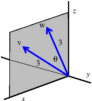 Problem 28
So we need to find vxw where v and w are vectors of length 3 in
the xz-plane oriented as in the picture, and the angle θ between
the vectors is π/6.
As I mentioned in class, when I first glanced at this problem I
thought that there was not enough information supplied to get the
answer. But let's think.
What is the direction of vxw? Please try to curl
the fingers of your right hand from v to w. I think if
you do, mentally at least (I tried to show it physically in class) the
thumb of your right hand will point in the direction of the negative y
axis. The direction should be –j, a negative multiple of j.
What is the magnitude of vxw? This should be
||v|| ||w|| sine of the angle between the vectors. We are
told that this angle is π/6 which has sine equal to 1/2. And each
length is 3. So the magnitude of the cross product is (3·3)(1/2)=9/2.
The direction should be backwards in y and the magnitude should be
9/2. The cross product therefore must be –(9/2)j.
Algebraic descriptions of lines and planes
Lines are discussed in the text on pp.689–690. Planes are discussed in
section 12.5.
Mostly I think I know what a line is and what a plane is. Here
is a picture with one of both of them displayed. But what happens if
we have several of them, and we want to deal very precisely with them?
It is useful, then, to have algebraic ways of describing and computing
with lines and planes.
| 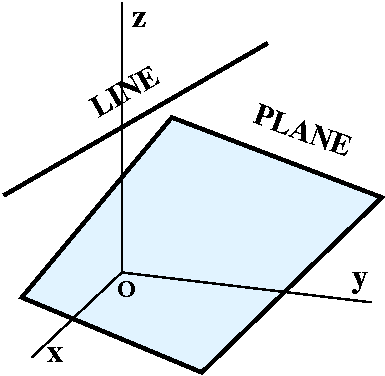 |
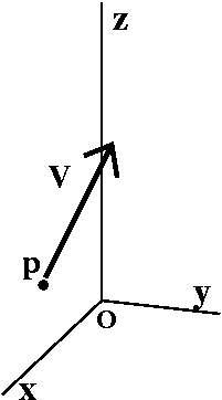 Specifying a line
The following information will usually be the most convenient way to
specify a line in this course:
- A point on the line (I'll call it p)
- A vector in the direction of the line (I'll call it v)
Then the line will be everything starting out at p going forward or
backward in the direction of v. More precisely, if q=(x,y,z), then q
will be on the line if the vector pq (from p to q) is a scalar
multiple of v. This might be easier to describe with an example.
Example
If p=(3,9,5) and v=<4,–7,6>, then the vector pq will be
<x–3,y–9,z–5>. Suppose t is a scalar. The
one vector equation pq=tv becomes the following three scalar
equations:
x=3+4t
y=9+–7t
z=5+6t
So these are parametric equations for the straight line
determined by the data p and v. Notice where the 3 chunks of p's
information go (no t's!) and where the 3 chunks of v's information
(the direction) go (with the t's).
Other parametric representations
I then played with these equations for a while. For example, the
equations
x=3+12t
y=9+–21t
z=5+18t
represent the same line. I just multiplied the direction v by 3. This doesn't
change the actual geometric line which is parameterized by the equations: every
point in "this" line is in the other line, and, similarly, the other way
around. And
x=3–4t
y=9+7t
z=5–6t
represents also the same line: I multiplied the direction by –1 but still
we will get the same total collection of points: the same straight line. And,
perhaps more complicated:
x=7+4t
y=–2+–7t
z=11+6t
This is also the same line. Notice, please, that the direction vector
is the same, but what I have changed is the "base point",
(7,–2,11). But if you consider the original parameterization, and put
t=1 in those equations, we will get (7,2,11). So, in fact, the
descriptions sort of "overlay" one another: the v's are the same, and
the we've just happened to start the parameterizations at different
points on the same line. In the next class, we will consider in detail
the kinetic aspect of the parameterization, but right now I tell you
that the lines (the collection of all the points described by these
triples of equations) are the same.
There is a plethora of different parameterizations for the same
straight line.
Plethora officially means "A superabundance; an excess."
Symmetric equations
Some manipulation gives another way to represent the line.
x=3+4t becomes t=(x–3)/4
y=9+–7t becomes t=(y–9)/(–7)
z=5+6t becomes t=(z–5)/6
so that we have (x–3)/4=(y–9)/(–7)=(z–5)/6. Such a collection of
equations is called the symmetric form of the line. As far as I know,
we won't describe lines this way in this course.
|
Two points determine a line
The original work of Euclid is available, translated and illustrated,
for free on the web. You may see here.
This work has been done by Professor Joyce of Clark
University. So, way back, thousands of years ago, Euclid decided
that a line would be determined by two points. How can we use such
information to get an algebraic description?
Example
Suppose p=(3,3,–9) and q=(–5,2,1). What are parametric equations for
the line through the points p and q?
The vector pq=<–5–3,2–3,–5–(–9)>=<–8,–1,4> is a vector in the direction of the line. We could use
either p or q (I'll use p here) for a "base point"
for the line. So we get the following parametric equations for the
line:
x=3+(–8)t
y=3+(–1)t
z=–9+(4)t
The colors are an effort to show where to put the data in the
parametric formulas.
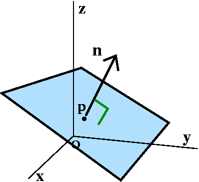 Specifying a plane
In this course, the data specifying a plane will also turn out to be a
point and a vector. What I'm about to describe may not look
immediately useful, but it will be, really. So what we will need is
- A point on the plane (I'll call it p)
- A vector
normal (perpendicular, orthogonal) to the plane (I'll call it
n)
I hope that a picture can be persuasive. There are many planes which
pass through the point p. But if you add on the requirement that, at
the point p, the vector n be perpendicular, exactly one geometric
"candidate" persists, and that's the plane I'd like to describe
algebraically.
What condition(s) on x and y and z will guarantee that q=(x,y,z) is on
the plane? We can look and conclude that the vector pq should be
perpendicular to n. We can check perpendicularity easily with dot
product. An example may help.
Example
Suppose p=(4,5,–7) and n is the vector <11,2,31>. The vector pq
is <x–4,y–5,z–(–7)> and pq is perpendicular to n exactly when pq·n=0. And that is
11(x–4)+2(y–5)+31(z–(–7))=0
This is a fine equation. You don't need to "clean it up". Of
course, it can be rewritten (if you must!) as
11x+2y+31z=44+10–217=163.
Again, there are many equivalent equations for one geometric plane
since there are lots of vectors normal to one plane, and lots of
points on one plane. And we can do the reverse:
Reversing ...
6x+–3y+7z=20 is the equation of a plane.
What is a vector normal to this plane? If you
followed the previous discussion, I hope you can see that the
components of such a vector are the coefficients of x and y and z in
order. So n=<6,–3,7> is a vector normal to this plane.
What are all (non-zero) vectors normal to this plane? These vectors
are the non-zero scalar multiples of <6,–3,7>.
What are the coordinates of a point on the plane 6x–3y+7z=20?
Part of the problem in answer this question is that there are so
many possibly answers! For example, (0,0,20/7) is one answer, and
so is (1,–7/3,1), and so is .... uhhh ... (1,000, –1,000,
–8,980/7). There are many points on the plane.
Three points determine a plane
Again, Euclid declared that 3 points in space should determine a
plane. So can we find an algebraic description of a plane through
the points p=(3,3,–9) and q=(–5,2,1) and r=(4,2,2)? We need to find a
vector n normal to the plane. The vectors pq and (say) qr are in
the plane's direction. The cross-product of these two vectors will be
perpendicular to the plane. So: pq=<–8,–1,4> and qr=<9,0,1>, and
   | i  j k |
det|–8 –1 4 |=–i–(–8–36)j–(–9)k=–i+44j+9k
   | 9  0 1 |
is a normal vector. So –1(x–3)+44(y–3)+9(z–(–9))=0 is an equation of this
plane. (We would get equivalent equations if we used q or r instead of p, or
if we computed with pqxpr instead of pqxqr.)
Supposedly (seeral thousand years olds!) "3 points in space
should determine a plane" but they may not always, because all 3 could
lie on one line. What then would happen to our vector algebra? Then
the two vectors we computed above would be scalar multiplies of one
another and the cross product which resulted would be 0. So we would
not be able to go on.
|
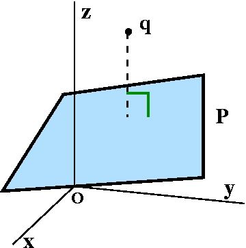 Distance of a point to a plane
Suppose the point q is not on a plane, P. How can we find the
distance from q to P? I did this in a rather clumsy way in class,
mostly because I wanted to practice how to use line and plane
equations. Let me start with specific information:
Suppose
q=(2,1,3) and P is the plane specified by the equation
5x–7y+6z=10.
First, is q on the plane, P? We can check this by substituting
the coordinates of q into the equation presented for P:
5·2–7·1+6·3=10–7+18=21, and 21 is not 10, so q is
not on P.
My strategy for finding the distance was to write the parametric
equations for a line through q perpendicular to P, see where the line
intersected P, and then compute the distance from q to that point. So
let me try to carry this out.
A line perpendicular to P through q We know that n=<5,–7,6> is a
vector normal to P. So
x=2+5t
y=1–7t
z=3+6t
are parametric equations for the desired line.
The intersection of the line and the plane Take the
parametric equations and plug them into the equation for the line:
5x–7y+6z=10 becomes 5(2+5t)–7(1–7t)+6(3+6t)=10 which is
(25+49+36)t=10–10+7–18 and this is 110t=–11 so t=–11/110=–1/10.
What does this value of t mean? It is the value of t which, when
substituted in the parametric equations, gives the intersection
point. So:
x=2+5(–1/10)=15/10
y=1–7(–1/10)=17/10
z=3+6(–1/10)=24/10
The intersection point is (15/10,17/10,24/10).
The distance between q=(2,1,3) and the intersection point
This is
sqrt{(2–15/10)2+(1–17/10)2+(3–24/10)2}. This
is sqrt(25+49+36)/10=sqrt(110)/10.
Another way ...
There are frequently different and equally valid solution strategies.
Here is another way to do this problem: (2,1,3) is not on the plane
5x–7y+6z=10. I can find a point on the plane just by "guess" (as I did
earlier, and I will guess for something convenient!): r=(2,0,0). Then
the vector rq=<0,1,3> points from the plane to q. Now if I project rq
onto the normal vector I will get a vector whose length is the
distance from the plane to the point. This "projection" is just what I
did last time when I found the parallel part of a
vector. So n=<5,–7,6> is still a vector normal to the plane. So we
just compute rq·n/||n||=(–7+18)/sqrt{110}=11/sqrt{110},
which is the same answer. This is more direct and more efficient and
if I had to do these computations many times a day, I would certainly
do this.
Parallel lines
I guess two lines are parallel if they are distinct (that is,
separate lines!) and if their directions are non-zero multiples of one
another. So, for example, the lines
Line A    Line B

x=5+t     x=30+t
y=3+2t    y=–9+2t
z=–1+3t   z=–1+3t
are parallel. Certainly their directions are multiples of one
another (the multiple is 1). But why are they "distinct"? The point
(5,3,–1) is on the first line. For it to be on the second line, uhhh ...
30+t=5, so t=–25. The second equation is then y=–9–(2)25=–59, and this is
not 3. So (5,3,–1) is not on the other line.
These are parallel lines.
|  |
Parallel planes
Two planes are parallel if they are distinct (that is, separate
planes!) and their normal vectors are non-zero multiples of one
another. For example, 2x+3y–z=56 and 4x+6y–2z=10 are parallel. Double
the first equation and get the right-hand side of the second: that
shows their normal vectors are non-zero multiples (the multiple is
2). But since twice 56=112 is not the same as 10, these planes are
definitely distinct: different.
|
 |
Skew lines
As dimensions increase, generally geometry gets more complicated. One
phenomenon which does not occur in two dimensions is skew
lines. A pair of lines is skew if they are not parallel and
also do not intersect. So look at, say, the x-axis (where parametric
equations could be x=t,y=0,z=0) and a line through (0,1,0) which is
tilted with respect to the x-axis: x=t,y=1,z=t. These lines don't
intersect since no point with second coordinate 0 is on the second
line. They aren't parallel since <1,0,0>, the direction of the first
line, is not a non-zero scalar multiple of <1,0,1>. So they are skew.
Things get even worse as n, the dimension, increases. For example, it
is possible to have pairs of skew planes (two dimensional
objects) in R4.
| 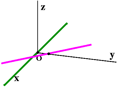 |
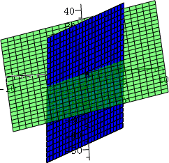 Intersection of two planes
The two planes 3x–y+z=4 and 4x+2y–z=7 are not parallel. They intersect
in a line. How can we get parametric equations for this line?
The planes are not parallel because the normal vectors
(<3,–1,1> and <4,2,-1>, respectively) are not scalar
multiples of one another. The planes are tilted differently. A Maple graph of these planes is shown to the
right. I hope you can see the intersection is a line.
A vector in the direction of the line will be perpendicular to both of
these normal vectors. The cross product gives us such a vector:
<3,–1,1>x<4,2,–1>
is
The QotD
The majority vote for the value of the cross product requested is
<-1,7,10>.
We also need a point on both planes. If x=0 then we must find y
and z which satisfy both –y+z=4 and 2y–z=7. I added the
equations and got y=11. Then students told me that z=15. (When you
first see this sort of thing it can be annoying, but there are
many points on the line, and unless I am very unlucky [the line
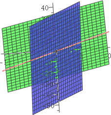 is perpendicular to the x-axis, for example!] I can just specify a
value for any one of the variables and then solve for the others!) So
(0,11,15) is on the line, and therefore a set of parametric equations
for the line is
x=0+–t
y=11+7t
z=15+10t.
To the
right is a picture of the two planes and the line of
intersection (in blue, green, and red respectively).
These pictures were drawn using the equations for the
two planes and the line. I did play with them a bit to get the
point of view shown, but not very much. I am not sure why the colors of the
planes in the two pictures are slightly different.
The principal commands used were plot3d,
spacecurve, and display, which are all in the package
plots. You will learn about this while
doing the Maple labs.
Parametric equations for a plane
Another way to describe a plane is parametrically. Pick a point
on the plane, and pick two vectors with distinct directions pointing
in the plane. Wait: let's look at an example. Suppose the plane
contains the point p=(9,–5,1) and the vectors
u=<3,–2,5> and v=<6,5,4> point along the plane (are
parallel to the plane, really). Then for all numbers s and t,
the points described by (9,–5,1)+su+tv describe a plane. I can
break this up into components:
x=9+3s+6t
y=–5–2s+5t
z=1+5s+4t
We will deal with this alternative algebraic description of planes
later when we discuss parametric surfaces. We can get back a
vector normal to the plane by taking the cross product of u and v.
|
Thursday, January 21, lecture #2
So the stunt I pulled on Tuesday (giving the first formal
"lecture" during the first recitation meetings) has given me
additional time to explain very intricate stuff at the end of the
course. I hope you will appreciate that later.
| ! | Special
Meeting Place |
! |
|---|
| Only on Tuesday, January 26, all
the recitations will meet in ARC 116 to learn about Maple. |
The easy (?) product
Suppose v=ai+bj+ck=<a,b,c> (the text uses these angle brackets,
and I will try to use them but probably I will get excited and replace
them with ordinary parentheses once in a while) and w=di+ej+fk. Then
I'll define the dot product or the scalar product or the inner product
(all of these phrases are used but I will mostly use "dot product") of
v and w to be the number
ad+be+cf
Our notation for this will be
v·w. Some textbooks use (v,w) or
<v,w>.
This doesn't look too impressive, but it turns out to occur enormously
frequently in many applications (so many, as I mentioned in class,
that most computer languages have devoted special attention to how to
evaluate it rapidly, and, indeed, the chips of many CPU's have special
"microcode" to evaluate inner products efficiently). Why would such
things occur in "real life"?
The farmer's market
New Jersey is the
Garden State. In the summer and early fall, almost every Friday I
go to a local farmer's market and buy fresh New Jersey fruits and
vegetables. So the task facing the cashier when I come up, hands full
of stuff, is to figure out what I owe. The logic of the cost
computation might be tabulated as follows:
| Type of purchase | Apples | Eggplant | Garlic | Onions | Peppers | Potatoes | Zucchini |
|---|
| Price per pound | $1.50 | $1 | $2.50 | $1.25 | $1.50 | $1 | 75¢ |
|---|
Weight of item
in pounds | 3 | 1.2 | .3 | 4 | 2 | 5 | 1.2 |
|---|
Now really look at the table. If you compute the total cost,
you'd better not confuse the order of the items. Each row has an
7-tuple of numbers: this is an element of R7. Let's call
the second row the cost vector, C, and the third row
will be the weight vector, W. What will the total cost
of this lovely purchase? Clearly it is
C·W dollars:
(1.5)(3)+(1)(1.2)+(2.5)(.3)+(1.25)(4)+(1.5)(2)+(1)(5)+(.75)(1.2).
I'm not particularly interested in the number, more in the logic.
A hobby or two?
Everyone should have a hobby, something silly to occupy their time
when they should be working. One of my hobbies, since I started
teaching calculus, is to go through a day and try to identify every
use of the derivative idea. There are lots and lots of them. Another
hobby, perhaps even more fruitful (pun intended!) is to identify every
darn use of inner product in a typical day. There are many uses. But I
am supposed to concentrate on three dimensions, so let's get back to
work.
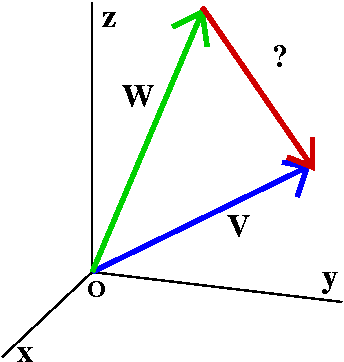 Looking at lengths again
Start with v=ai+bj+ck so that
||v||=srqt{a2+b2+c2}. If w=di+ej+fk,
then ||w||=srqt{d2+e2+f2}. If I draw
the vectors v and w with their tails on the origin, then a vector,
identified in the picture with "?", completes a triangle, going from
the head of w to the head of v. Rhat vector isn't too mysterious. I
know that w+?=v, so ?=v–w. In terms of components, we can write
v–w=(a–d)i+(b–e)j+(c–f)k. The length of
v–w is
sqrt{(a–d)2+(b–e)2+c–f)2}. You
can check easily that the length of v–w and the lengths of v and
w are not related in any simple way.
Really the squares of the lengths
With all the square roots, maybe we should be looking at the squares
of the lengths. Also the algebra will be easier!
Then
||v||2=a2+b2+c2 (this is
the same as v·v, the dot product of
v with itself)
and ||w||2=d2+e2+f2
and
||v–w||2=(a–d)2+(b–e)2+(c–f)2.
We can "expand" the last term to get
||v–w||2=a2–2ad+d2+b2–2be+e2+c2–2cd+f2.
That is exciting.
The obstacle to making it work
If you compare terms, the sum ||v||2+||w||2 is
the same as ||v–w||2 except for
–2ad–2be–2cf=–2(ad+be+cf). So computations
with lengths and squares of lengths will have to include that
"mess". Let me forget the –2, which isn't that essential. What
an accident: the obstacle to making things ridiculously simple is
(essentially) the dot product.
The law of cosines lurks ...
There's a formula which generalizes the Pythagorean Theorem's
formula. For the triangle shown above, here it is:
||v–w||2=||v||2+||w||2–2||v|| ||w||cos(θ)
Here θ is the angle opposite the side v–w. If θ is Pi/2, the
cosine term is 0 and we get back Pythagoras. Here is the geometric view of the areas of
the squares on the sides of a triangle.
The geometry of the dot product
Since we know that
||v–w||2=||v||2+||w||2–2||v|| ||w||cos(θ)
and we know that
||v–w||2=a2–2ad+d2+b2–2be+e2+c2–2cd+e2=||v||2+||w||2–2v·w. We
see that (cancelling the –2's)
v·w=||v|| ||w||cos(θ) where θ is the angle between v and w.
Notice that we can now see if v and w are not 0, then v and w are
orthogonal (perpendicular, normal) exactly when v·w=0.
Determining an angle
Suppose v=<3,2,–1> and w=<5,2,6>. What is the angle between v and w?
We compute: v·w=15+4–6=13, ||v||=sqrt(14), and ||w||=sqrt(65). Therefore
cos(θ)=13/[sqrt(14)sqrt(65)]. This gives approximately
(calculator-assisted computation here!) 64.55 degrees or (better, I
guess) 1.126 radians.
Resolving a vector into perpendicular and parallel parts
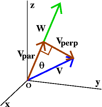 Let me continue using the v=<3,2,–1> and w=<5,2,6> from the previous
question. I'd like to show you how to write v as a sum of two
vectors, v|| and v⊥ where v⊥
is perpendicular to w and v|| is parallel to w. This will
be useful several times in the course, and is also important in
physics.
How long is v||? If you look at the picture, the
v|| is part of a right triangle. It is the adjacent leg and
v is the hypoteneuse. Θ is the angle between them. Therefore
||v||||=||v||cos(θ)=v·w/||w||. We did some of these
computations just above, so ||v||||=13/sqrt(65). How can we
get the correct direction? So we want a vector whose length is
13/sqrt(65) and whose direction is the direction of w. We can
create a unit vector (a vector of length 1) in the direction of
w: that will be w/||w|| which is <5,2,6>/sqrt(65). And now we adjust
this unit vector by stretching it, to get
[13/sqrt(65)]<5,2,6>/sqrt(65). This is about all I did in class, but
let me finish things here. The vector is
(13/65)<5,2,6>=<1,26/65,78/65>. Since
v=v||+v⊥, we know that
v⊥=v–v||=<3,2,–1>–<1,26/65,78/65>=<2,104/65,–143/65>.
Checking the answer
v⊥ should be perpendicular to w. So let's
compute v⊥·w=<2,104/65,–143/65>·<5,2,6>=10+(208/65)–(859/65)=(650+208–858)/65=(858–858)/65=0,
so these vectors are indeed orthogonal.
Comment I admit (informative to you and irritating to me) that
I did all these computations by hand, and I had to do them three
times to get them to come out correctly. The computation here
occurs frequently in some elementary physics applications, and is the
beginning of a rather profound and widely used algorithm in linear
algebra called the Gram-Schmidt process.
The dot product and its basic properties
If v=ai+bj+ck and w=di+ej+fk, then v·w=ad+be+cf.
The dot product obeys the following algebraic rules which are not
difficult to check but the details are tedious.
- If v and w are vectors then v·w is a
scalar (in this course this means "a real number").
- (Commutativity) v·w=w·v. (You can see this is correct by
looking at the pieces of v·w and
w·v. For example, ad is the same as
da.)
- (Linearity or distributivity of vector addition over scalar
multiplication) (v1+v2)·w=(v1·w)+(v2·w). (Again, you can check that this is
correct by doing algebra with the components. A similar statement is
true about the second factor, sice dot product is commutative.)
- v·0=0.
- v·v=||v||2.
Color change?
I'll write material with this background color if I just did not have
time to discuss it in class but if I think it is useful enough that
students might profit from seeing it.
Example with a little table
Suppose we have four rambunctious ("Boisterous and disorderly")
vectors: v1 and v2 and w1 and
w2. Suppose also we have this little multiplication
table for their dot products:
 · | w1 | w2
--------------
 v1 | 3  | 7
--------------
 v2 | 4  | –2
Could we then compute something like
(4v1–3v2)·(5w1–2w2)?
Here I would expect people to distribute or take advantage of linearity on
both the left- and right-hand sides. The process might
go like this:
(4v1)·(5w1–2w2)+(–3v2)·(5w1–2w2)
(4v1)·(5w1)+(4v1)·(–2w2)+(–3v2)·(5w1)+(–3v2)·(–2w2)
(4·5)v1·w1+(4·–2)v1·w2+(–3·5)v2·w1+(–3·–2)v2·w2
(4·5)(3)+(4·–2)7+(–3·5)(4)+(–3·–2)(–2)
And the answer seems to be .... 60–56–60–12=–68. I think this is
correct. I make more errors in such computations when no one is
watching me.
|
Another product, introduced geometrically
I defined the dot product by a rather simple algebraic formula. The
cross product has a complicated algebraic formula, and maybe it is
easier to begin by defining it geometrically.
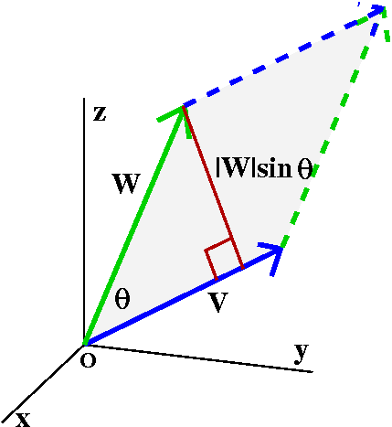
The cross product (also called the vector or outer product) takes two
vectors, v and w, and produces vxw, another vector. Since this is a
vector, it is specified by its magnitude and direction.
Magnitude of vxw
Look at the the vectors v and w. There is a parallelogram which has
sides v and w. The area (a non-negative quantity) of that
parallelogram is the magnitude of vxw.
There is an easy formula for the area in
terms of the lengths of the vectors and the angle between them (you
get it from using the base times the altitude, where the base has
length one of the vectors and the altitude is sine multiplied by the
length of the other vector). The
area is ||v|| ||w||sin(θ). You get this by multiplying the base
by the altitude in the plane of the parellelogram.
Direction of vxw
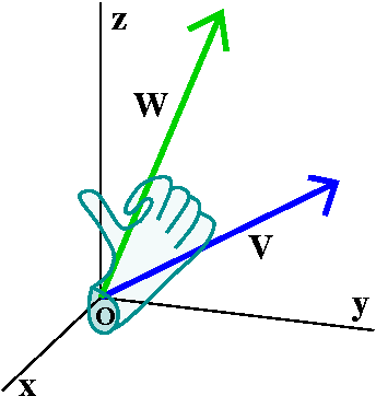 Take your right hand and extend your
thumb. Curl up your fingers. Insert your hand (I guess by thought, not
physically) so that your fingers go from v to w. Then
your thumb will be (sort of) pointed perpendicular to the plane
containing v and w. That perpendicular direction is the direction of
vxw.
The only reason that such a weird product would be considered is that
it is useful. We will see some geometric uses of it in this course and
most of you will see uses in mechanics (torque), eletromagnetism,
fluid flow, etc.
The i,j,k multiplication table
So before anyone could yell too much I computed the cross product
"multiplication table" for i and j and k.
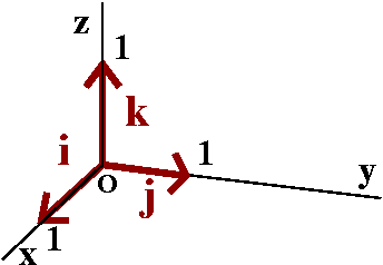 This wasn't too hard,
although getting the directions correct involved some thought
and some physical contortions. These are unit vectors and all mutually
perpendicular. If the vectors in the product are the same, then the
parallelogram involved collapses to a line segment and has no area. If
the vectors are different, then the parallelgram is a square with 1
unit sides, and has area 1. The important thing is the sign of the
answer and its direction. I tried to get that correct. If you were not
in class or you were confused, I urge you to try to get some of the
entries in this table yourself.Then the cross product in terms of components is
 x |  i  |  j  |  k
--------------------
 i |  0  |  k  | –j
--------------------
 j | –k  |  0  |  i
--------------------
 k |  j  | –i  |  0
Weird stuff
Things to notice:
ixj=k and jxi=–k. The cross product is not
necessarily commutative. In fact, the cross product is
anti-commutative:
vxw=–wxv always.
(ixj)xj=kxj=–j and ix(jxj)=ix0=0. The cross product is not
necessarily associative.
This means that you can't necessarily rearrange or regroup cross
products. This is annoying. The cross product does not resemble many
other products you have seen.
Then the cross product in terms of components is ...
I then did the following awful computation, which you should never do:
If v=ai+bj+ck and w=di+ej+fk, then vxw=
(ai+bj+ck)x(di+ej+fk)=ad(ixi)+ae(ixj)+af(ixk)+bd(jxi)+be(jxj)+bf(jxk)+cd(kxi)+ce(kxj)+cf(kxk).
I filled in all the values from the multiplication table above and got
the following mess:
vxw=ad(0)+ae(k)+af(–j)+bd(–k)+be(0)+bf(i)+cd(j)+ce(–i)+cf(0)=(bf–ce)i+(cd–af)j+(ae–bd)k
This last formula can be expressed in a very neat way if you know about determinants.
It turns out that | i j k |
vxw=det| a b c |
| d e f |
here's a very brief discussion of determinants in the textbook. I
will probably evaluate this determinant most of the time by "expanding
along the first row" but you may use any valid method.
Why is what I've done correct?
The definition I gave for cross product was geometric. Some of the
properties of cross product are easy from the geometric
definition. But I've just used linearity (or distributed the sum over
the cross product), something like this:
(v1+v2)xw=(v1xw)+(v2xw). Why is this true? This is not clear (!) to me at all from the
geometric definition. Here
is a paper which shows why you can distribute using geometry. Figure 8
on page 9 of this paper is a picture which should convince (is
supposed to convince) you that cross product does have the desired
algebraic property. I hope you will find it convincing. I find it
difficult to really understand.
|
QotD
Compute v·w and vxw if v=<2,1,3> and w=<3,0,–4>.
The dot product is –6 and the cross product is –4i+17j–3k
Tuesday, January 19, lecture #1
Mr. Nanda will usually teach the recitations. He could not
be present today. The course covers so much material that I was
reluctant to lose time, so I just gave the first lecture three
times. Sigh. Now I am very tired. The idea was good,
because now I have an additional lecture to discuss much more
complicated material occurring later in the course. But I am just a
bit tired.
Who am I?
I'm a faculty member in the Rutgers Math Department. Much of my
professional work has involved differential equations involving
functions of more than one variable. I actually like the
content of this course, and I may get almost incoherent with
excitement and pleasure when describing some of the subject
matter. Certainly I will draw pictures that seem to mean something to
me, but they may be totally incomprehensible to almost everyone
else. I apologize in advance.
Diary
I will try to write a diary for this course, since some
students have told me it is helpful. I will use
lots of material from the diary I wrote the last time I taught
251. This is not "plagiarism". I wrote the material, I acknowledge
using it, and I've given myself permission. For your information, it
isn't usually the text that takes much time, but rather the darn
pictures. Lots of time is needed to create good pictures!
Who are you?
Many of the students in these sections are
engineering students. Many engineering students (especially in
Mechanical, Chemical, and Biochem) will go on to take Math 421 where
all the material of this course is used. Other students are from such
disciplines as chemistry, computer science, mathematics, meteorology,
and physics. Certain biological science majors take this course,
principally because they will take physical chemistry, and the
language of several variable calculus is essential in
pchem. Additionally, some students may be in this class for "fun" (if
that's possible) but may be interested in a business career. It turns
out that there's a huge developing field of mathematical finance and
the ideas of this course are, again, essential tools.
What will we study?
I tried to briefly discuss the background of the
course. The link indicated has more information.
Then we went on to "review" analytic geometry of one and two and even
three dimensions. I put the word in quotes because most students who
have taken courses in applied science and engineering have already
seen the material we will discuss in 2 or 3 or even 4 other courses!
The poor math majors may never have seen this before so they
especially should read the text.
R1
 This is supposed to be the real line. There's an origin and a
unit length, and the conventional choice is to make the positive
direction go off to the right. Each point on the line corresponds to a
real number. The distance between points on the line which correspond
to the real numbers a and b is defined to be |a–b|.
R2
 And here is the plane (I don't think I've ever heard anyone
call it the "real plane"). The simplest situation is what's shown
here. Two straight lines as axes, perpendicular to each. Every point
corresponds to a unique ordered pair of real numbers. There is a set
unit length on each coordinate axis, and almost always right is
positive and up is positive. Later in the course we will consider
situations where the coordinate axes are not necessarily
perpendicular. And even where what corresponds to the axes are not
straight. I hope that tilted axes could make sense if, for
example, you were interested in looking at crystals which did not have
rectangular symmetry. I used Pythagoras to deduce the distance formula
giving the distance between two points in the plane.
R3
 In three dimensions, the standard geometric situation is specified by
three mutually perpendicular lines. Points will correspond to ordered
triples of real numbers. In almost every situation you are likely to
encounter, these axes will be right-handed. Right-handed means
... means ... means ... it means what I sketched to the right (heh
heh). The three dimensional world is complicated, and you will see
that the choice of right-handedness has some interesting consequences.
Chirality or handedness
A discussion of Chirality is linked.
Here is a short
discussion of parity in chemistry and physics. And here is a Wikipedia
article on enantiomers, which are compounds that are
non-superimposable mirror images of one another. This article is a bit
more technical, but has many examples of pharmaceutical products which
are mirror images.
Perilous pictures
Here is my attempt to draw the point with coordinates (3,2,–1).
The green "path" with  's sort of tells how to find the
point. I walk (?) from (0,0,0) to (1,0,0), then to (1,3,0), and
finally to (1,3,–2). Each 's sort of tells how to find the
point. I walk (?) from (0,0,0) to (1,0,0), then to (1,3,0), and
finally to (1,3,–2). Each  is
supposed to represent one unit of the path. I think that the
complications of perspective and reducing the "object" from three
dimensions to a two-dimensional representation may make even such a
simple picture difficult to understand. If you weren't told that the
point was supposed to be (1,3,–2), would you have guessed those were
the coordinates? Sigh. is
supposed to represent one unit of the path. I think that the
complications of perspective and reducing the "object" from three
dimensions to a two-dimensional representation may make even such a
simple picture difficult to understand. If you weren't told that the
point was supposed to be (1,3,–2), would you have guessed those were
the coordinates? Sigh.
I will try to draw good pictures, but I won't always
succeed. And even if I draw pictures which I believe are suitable, you
may not agree. Pictures are complicated and sometime personal.
|
|
Some simple geometry and equations
What points in R3 have y=2? Certainly (0,2,0), on
the y-axis, is the only point on the y-axis with y=2. We can move up
and down (changing the z-coordinate) and sideways (changing the
x-coordinate). We can even change both. The collection of points we
get is a plane, perpendicular to the y-axis through the point
(0,2,0). An attempt at a picture is to the right. You don't need to
agree that this is a good picture.
In this course I will probably regard the following technical words as
synonymous (the words mean the same) most of the time:
perpendicular
orthogonal normal
|
|
|
What points in R3 have z<5? This is a an open
half-space. The plane z=5 is the boundary of this region and
the region does not include the boundary. Later in the course I'll try
to discuss the use of "open" and "boundary" in more detail. Here the
boundary is a plane normal to the z-axis through the point
(0,0,5). The plane, however, is not included in the region
specified by z<5. What I've attempted to show in
the picture is an open half-space.
|
|
| Let's imagine a brick in R3 with its
sides parallel to the xy and yz and xz planes. Maybe this could be
called a right-angled parallelopiped. Suppose one corner (also called
a vertex) has coordinates (a,b,c) and the diagonally opposite corner
has coordinates (d,e,f).
|
 |
Now let's look at the corner displayed in the
accompanying picture, the corner illustrated with  . What are the coordinates of that
point? . What are the coordinates of that
point?
If you can "see" what the picture is supposed to show, then the
designated corner is just moved "out" parallel to the direction of the
y-axis. The x-coordinate doesn't change at all, and the height from
the xy-plane (which is the z-coordinate) also doesn't change.
Therefore the coordinates of  are
certainly (a,?,c). What about the second coordinate of the
point? If you look at the picture with me, you can see that the entire
face or side of the solid between are
certainly (a,?,c). What about the second coordinate of the
point? If you look at the picture with me, you can see that the entire
face or side of the solid between  and the point (d,e,f) has constant y-value: it is
perpendicular to the y-axis. Therefore the mystery middle coordinate
must be the same as the middle coordinate of (d,e,f), and so and the point (d,e,f) has constant y-value: it is
perpendicular to the y-axis. Therefore the mystery middle coordinate
must be the same as the middle coordinate of (d,e,f), and so
 =(a,e,c). =(a,e,c). |
 |
Now let us play the same game with another
vertex (or corner). So the designation of  has been
moved to the corner shown. What are the coordinates of this point?
This point is on the same face or side of the solid so it certainly
shares the second or y-coordinate with both (d,e,f) and (a,e,c), so has been
moved to the corner shown. What are the coordinates of this point?
This point is on the same face or side of the solid so it certainly
shares the second or y-coordinate with both (d,e,f) and (a,e,c), so
 =(?1,e,?2). The third
coordinate, ?2, must be c since the point we're
looking at is certainly on the bottom face of the solid. The first
coordinate might be the most puzzling, but both (d,e,f) and =(?1,e,?2). The third
coordinate, ?2, must be c since the point we're
looking at is certainly on the bottom face of the solid. The first
coordinate might be the most puzzling, but both (d,e,f) and  are on the
"back" face (that is part of the plane x=d) of the solid, so the
x-coordinate we're looking for is d. Therefore this are on the
"back" face (that is part of the plane x=d) of the solid, so the
x-coordinate we're looking for is d. Therefore this  is
(d,e,c). is
(d,e,c).
A good exercise for you is to figure out the coordinates of
some of the other corners of the brick.
|
 |
| Now I'd like to compute the length of some of the edges of the
brick. For example, what is the length of the line segment connecting
(a,b,c) and (a,e,c)? This is the distance between these two
points. Notice that the only coordinate which is varying is the middle
one. This side is a line segment which is parallel to the y-axis. We
can measure length along it only by thinking about the
one-dimensional distance between b and e. That distance is |b–e|. The
reason for the absolute value signs is that distance is supposed to be
non-negative.
|
|
| We can try to do the same thing with the edge connecting the
points with coordinates (a,e,c) and (d,e,c). Here the only coordinate
difference is in the first, x-, coordinate. So distances again should
be measured as if they were in one dimension, along the parallel
x-axes. The distance we want is |a–d|.
|
|
Now we can be even more bold. (Bold for a math class.)
We can find the distance from (a,b,c) to (d,e,c). Look carefully
and see that there is a right triangle whose hypotenuse is the
distance wanted, and whose "legs" have distances we already know. Then
Pythagoras declares that the length of the hypotenuse is
sqrt(|b–e|2+|a–d|2)
If
you are somewhat alert this result is not too surprising. The bottom
face of this brick is where z=c. The formula written is just the
ordinary two-dimensional distance between the points (a,b) and (d,e).
|
|
I'm not going to try to put that formula in the picture. I
will just label the distance Blah. Now I want the distance
along one of the main diagonals of the brick, from (a,b,c) to
(d,e,f). There is, as shown, another right triangle. The hypotenuse is
the distance I want, and the two legs have distances we know: one is
Blah and the other is ... the other is: the same ideas as
before (since the endpoints differ in only one coordinate) tell me
that the distance is |c–f|. Therefore (again Pythagorus) the
distance between the farthest apart corners is
sqrt(Blah2+|a–d|2)
But let me write it out in all of its glory (or gory [details, that is!]):
|
 |
sqrt({sqrt(|b–e|2+|a–d|2)}2+|a–d|2)
Here I inserted the formula we previously got for Blah. But
lots of what is written in this formula is superfluous. The square of
a square root is always the number. We don't need absolute values if
we are square a number. So therefore we can make a spontaneous (!)
definition:
The Euclidean distance
The (Euclidean) distance between (a,b,c) and (d,e,f) is sqrt((a–d)2+(b–e)2+(c–f)2).
A bunch of comments
First, math definitions shouldn't (and generally aren't) written at
random. They ideally should be supported by examples and
"intuition". Here the word intuition really means looking at lots of
situations and extracting the important common ideas.
In this course you'll observe an enormous storm of
definitions. Almost all of them are not motivated by anything
resembling "theoretical" considerations. The definitions were created
to help discuss various real physical and geometrical situations. So
the fact that the math is widely used in so many applications is not
an accident -- it was arranged that way!
Second, the definition actually shows you how to define distance
between points in R17, if you would ever want to. The
definition should be something like the square root of the sum of the
squares of the differences between the respective coordinates of the
points. And this actually (for many purposes) is a good definition.
The distance between two points is 0 exactly when the points are the
same, and the distance between p and q is the same as the distance
between q and p. Math majors who have taken Math 300 might recognize
the skeleton of a definition using mathematical induction. But I can't
talk about this here.
I remark that the distance defined is called the Euclidean
distance because there are other ways of defining "good" distances,
and some of them are useful in other contexts. Students who study
digital signal processing will find out that the Euclidean distance is
perhaps not always the most useful distance when comparing signals. In
this course, the Euclidean distance will be the only one used, so I
will almost always omit the adjective "Euclidean". What is nice about
the Euclidean distance, though, is that it is very computationally
neat, and leads to the method of least squares, which is a very
commonly used method of fitting "curves" (function descriptions) to
data points.
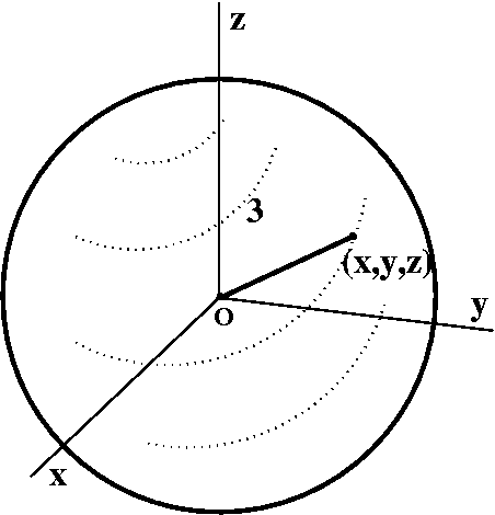
A sphere of radius 3
What algebraic condition on a point (x,y,z) is equivalent to the
geometric statement that the point lies on a sphere of radius 3
centered at (0,0,0)? This means that the distance from (x,y,z) to
(0,0,0) should be 3, or
sqrt((x–0)2+(y–0)2+(z–0)2)=3 which of
course is the same as x2+y2+z2=9.
Completing the square to "recognize" a sphere
We could of course "reverse" the process if we're given an equation
(or at least an equation of the correct form). So the equation
x2–3x+y2+4y+z2–7=0
represents a sphere. What is its center and its radius? The key
algebraic maneuver here is completing the square, and
everything works very much as in two dimensions.
x2–3x →
x2+2(–3/2)x →
x2+2(–3/2)x+(–3/2)2–(–3/2)2 →
(x–3/2)2–(–3/2)2
y2+4y →
y2+2(2y) →
y2+2(2y)+22–22 →
(y+2)2–22
We don't have any term with z to the first power. So the equation
becomes:
(x–3/2)2–(–3/2)2+(y+2)2–22+z2–7=0
which is the same as
(x–3/2)2+(y+2)2+(z–0)2=(–3/2)2+22+7
and we can "read off" that the center is (3/2,–2,0) and the radius is
sqrt((–3/2)2+22+7). It is easy to make mistakes
with minus signs when identifying the center. It is also easy to
forget to take the square root when identifying the radius. Oh well.
If we had different (but positive) numbers in front of the squares
(x2 and y2 and z2) then we'd get an
egg-shaped object, an ellipsoid. We'll see more about this
later.
Vectors
A vector is a directed line segment. It is used as a
mathematical model for any quantity which has both magnitude and
direction. Here are some quantities which are vectors
and some which are not:
|
|
Some vector quantities
Acceleration, velocity, displacement For velocity, for
example, the length of the vector corresponds to speed: "I am
traveling at 25 miles per hour" (in metric, I think that is 78
hectares per wombat). Of course the direction of the vector
corresponds to the direction of motion: "I am traveling at 25 miles
per hour North by Northwest" (in the metric system, this direction is
called "Colder").
Force Another basic example of a vector. The magnitude is
the amount of oomph in the force (I am giving up on units) while the
direction is the direction the force is pushing in.
Moment, torque, etc. You'll meet lots of vector
quantities. |
Things which aren't vectors
Mass (=energy, according to our good friend Albert).
Temperature
Quantities which are not vectors have the strange adjective,
scalars. So both Mass and Temperature are scalar quantities, and are
measured by numbers (both positive and negative) and have no intrinsic
direction.
|
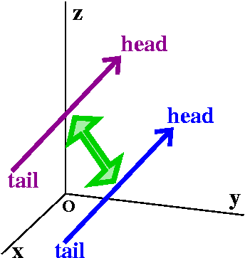 Equal vectors
A vector can also be specified by its head and tail.
Two vectors will be called equal (maybe the official word is
equivalent) if when the tail of one of them is moved to the tail of
the other, then their heads are in the same place.
Vectors are used to do algebra in more than one dimension. This is
because algebra has really been successful, and the interaction
between algebra and geometry has paid off in both
directions. Therefore we'll need to add and multiply vectors. Efforts
to multiply run into serious difficulties, as we will see next
time. Addition is neat and "everything" works. As I mentioned in
class, the generally accepted definition for vector addition models
some situations which can be experienced and measured in "real life"
with forces, velocities, etc. The word resultant is sometimes
used in connection with this definition.
Definition of vector addition
| First suppose there are two vectors, v and w, which are
roaming, free and happy in R3. |
We take the vector w and drag it so that the tail of w is at
the same point as the head of v. |
The vector v+w is now defined using the geometric display we just
arranged. v+w the vector whose tail is at the tail of v and whose head
is at the head of w.
|

|
Properties of vector addition
- Reality Addition (superposition, resultant) of
vector quantities in physical "reality" is modeled by vector
addition. As I mentioned in class, there probably are many ways
we could define vector addition. This way is used because it
accurately models certain physical situations. Please keep this in
mind!
- Commutativity v+w=w+v for all pairs of vectors v and
w.
This can be proved from the geometric definition by drawing a
parallelogram which has one pair of sides translates of v and the
other pair of sides translates of w. Anyway, the order in which you
add vectors doesn't matter.
- Associativity (v+w)+u=v+(w+u) for all triples of vectors v,
w, and u.
I think this can be proved by drawing some
parallelopided (three-dimensional analogue of a parallelogram) with
sides gotten form v and w and u: but the diagram would almost be more
annoying than just thinking about it. The important consequence is
that you can group adding vectors in any way you want, and the result
will be the same.

Zero and minus
The zero vector has its head equal to its tail. If v is a vector, then
–v is the vector whose length is v's but whose direction is the
reverse: so the head of –v is the tail of v and the tail of –v is the
head of v. Huh. Say that fast.
I am especially proud of the image of the zero vector in the picture
to the right. I wanted to show the special beauty of the zero
vector. I tried several different angles. (This is a joke!)
Then v+(–v)=0, and v+0=0 etc. for all vectors.
Scalar multiplication
In this course the scalars will be real numbers. Scalars are
things that multiply vectors. Many of the students in the course will
see later situations where the scalars are complex numbers. In the
case of the vectors arising in computer science and electrical
engineering, collections of scalars occur which are much less
familiar.
If c is a scalar and v is a vector, then the vector cv is defined by
the following:
If c>0 the direction of the vector cv is the same as the
direction of v, and the length of cv is the length of v multiplied by
c.
If c=0 then cv is the zero vector.
If c<0 the direction of the vector cv is the same as the
direction of –v and the length of cv is the length of v
multiplied by |c|. (The absolute value makes sure that lengths stay
positive.)
Here are pictures of v and –v and 3v and –2v.

Important vectors
Some vectors are more important than others, especially if you have a
coordinate system. The vectors i and j and k are vectors of length 1
(such vectors are called unit vectors) which are parallel to
the coordinate axes x and y and z, respectively.
|
 |
Now take any vector v and move it so that the tail of v is at the
origin, (0,0,0). Then the head of v will be at some point, (a,b,c). If
you think about the geometry I hope you can convince yourself that
v=ai+bj+ck. We have written v as a sum of its components.
The textbook also uses the notation v=<a,b,c> for this. |
 |
Vector addition in terms of components
Since vector addition is commutative and associative, and certainly
(c1+c2)(any vector)=(c1)(that vector)+(c2)(that vector),
we see clearly that if v=ai+bj+ck
and w=di+ej+fk, then v+w=(a+d)i+(b+e)j+(c+f)k.
The components of the sum are the sum of the respective components.
If you know the components, it is easy to compute vector sums and
scalar multiples of vectors.
The head and the tail produce the vector (algebraically)
Suppose the point P has coordinates
(x1,y1,z1) and the point Q has
coordinates (x2,y2,z2). Then the
vector from P to Q (so P is the tail and Q is the head) is just
(x2–x1)i+(y2–y1)j+(z2–z1)k.
I hope that you can draw a picture convincing yourself of that,
or you can look in the text.
Example The vector from P=(1,2,–3) to Q=(–5,6,2) is
(–5–1)i+(6–2)j+(2–[–3])k=–6i+4j+5k. It is easy to make mistakes with
signs in this computation.
How long is a vector?
I will use length and norm and magnitude to mean
the same thing about a vector: its length. If v=ai+bj+ck, then we can
think of the tail of v as sitting at (0,0,0) and the head of v, at
(a,b,c). The length formula we got then says that the length must be
sqrt(a2+b2+c2). So if you know the
components, the magnitude can be computed. In the textbook we are
using the magnitude is written ||v||. Please note that in some books
and some situations, this quantity is just written |v|.
NO! NO, NO, NO!!!
Suppose that v=<1,2,3> and w=<–2,3,2>. Then v+w=<–1,1,5>. And
||v||=sqrt(14) (approximately 3.74), ||w||=sqrt(17) (approximately 4.12),
and ||v+w||=sqrt(27) (approximately 5.19). In general, these numbers
need not be related in any simple fashion, aside from the Triangle
Inequality (see the textbook, please).
Next time I will explore how these lengths can be explained,
as we discuss multiplication of vectors.
Start reading chapter 12, please. Do the problems.
Maintained by
greenfie@math.rutgers.edu and last modified 1/19/2010.
 The points in R3 which satisfy
x2+y2+z2=R2 are a sphere
of radius R centered at (0,0,0). We could say that z is defined as a
function of x and y by this equation. In fact, since the situation is
relatively simple, we can actually solve for z in terms of x
and y:
z=±sqrt(R2–x2–y2). From
this equation we can compute ∂z/∂x etc. But if we assume
that z is defined implicitly as a function of x and y by the
equation, we can compute using the Chain Rule by just
∂/∂x'ing the whole equation:
 If we take a long "homogeneous" rope, and wiggle it a bit, the wiggles
propagate down the rope. It turns out (neglecting units,
neglecting certain other hypotheses, but keeping the central idea)
that for small wiggles, if we define f(x,t) to be the height of the
rope at position x and at time t, then
  No, I don't really need to "write" the 1's
but I want you know that
they are there: the Chain Rule was used. Now again:
 My online dictionary states that a nebula is "a cloud of gas
and dust, sometimes glowing and sometimes appearing as a dark
silhouette against other glowing matter." So we could pilot a
spaceship through a nebula. We might be concerned about the physical
effects of the nebula, for example, the temperature. I'll assume that
the spaceship measures temperature at the tip of its front. A point in
the nebula will be located with rectangular coordinates, (x,y,z). The
temperature at that point will be T(x,y,z). The rocket will fly a path
so that at time t its location will be <x(t),y(t),z(t)>.
  Observation 3
 A better example (!)
 Tangent planes


 The QotD: tangent plane to an ellipsoid
 Slicing and partial derivatives
 So F is a solution of the Heat or Diffusion Equation
 A really silly (?) two-variable example
 By the way, if you don't like piecewise defined functions, you could
consider the function defined by this formula:
f(x,y)=xy/sqrt(x2+y2). It has properties which
are similar to the piecewise function, but it is a bit harder to
analyze. You could look at it using Maple, and then you might get some insight.


 Here is one of the variations which can be produced with the plot3d command. It has the three-dimensional
(the two-dimensional picture of the three-dimensional graph!) plot
with the contour lines shwon at the correct places on the graph. There
are all sorts of views which can be obtained using the options of
plot and plot3d . Sometimes these variants can be
useful.


 Two half planes
 The contour "lines"
 Now comes some of the harder stuff. I asked people to imagine that
some bugs were "walking" on the graph of z=f(x,y). The green bug, whose path is shown to the
right, strolls along in a path which is roughly circular around the
origin. This bug runs into trouble at any point on the positive
y-axis, where there's a drop. It also has problems along the negative
y-axis, where again there is a big difference in heights. This is a
very small bug. I have tried to indicate this by a sort of light
reddish color surrounding these half-lines. The
blue bug walks from the right halfplane to the left
halfplane. It is careful to cross only at the origin. The blue
bug is totally safe, and never comes across any severe height
differences. So I would like to discuss (and name [define], since it
is a math course!) the differences the bugs encounter more precisely.


 The final example of misbehavior was the following function:
 Let's define the unit tangent vector, T, to be a unit vector in
the direction of r´(t), the velocity vector. If θ is the
angle that r´(t) makes with the positive x-axis, then T must be
cos(θ)i+sin(θ)j. Also r´(t)=(ds/dt)T, where ds/dt,
the speed, is the length of r´(t). Now differentiate the formula
for r´(t) using one of the product rules we had stated earlier.

 Now a more complicated thought experiment. Imagine the ball bearing
constrained to move in a piece of a circular tube. All we know is that
the object is moving, and its motion is part of a circular arc. I
claim that then, no matter what, the ball bearing is "feeling"
a transversal (normal) force from the "walls" of the tube. Why? The
normal component of the acceleration (a scalar multiple of the force
acting on the object) is κ(ds/dt)2. κ is not 0
since it is 1/(radius of the circle). And, since the object is moving,
we also know that ds/dt is not 0. Therefore the product isn't 0, and
the normal component of the acceleration isn't 0. There is
always a normal force.


 I hate to leave this subject since there is much more to be told, and
everything turns out to be amazingly useful in a wide variety of
applications. I hate to leave the subject, but the course is very
dense. So: a little bit more. Think of an airplane flying along a
curve in the sky (the dashed red line). Then the unit tangent and
normal vectors are as shown. There's another vector, B, called the
binormal vector, which is TxN. Since T and N both have
length 1 and they are perpendicular, then B also has length 1 (sine of
a right angle is 1). And B is perpendicular to both T and N.
 QotD
QotD Curvature is a number which measures how a curve bends


 A racetrack: this racetrack consists, as nearly as possible, of two
straight line segments, each about 3 miles long, connected with a
semicircular track. Since the racetracks were specified to be 2 miles
apart, we "deduce" that the radius of the semicircle is 1 mile. The
racetracks certainly have curvature=0, and the semicircle, which is
Π units long, has curvature 1. What would a graph of the curvature
of this racetrack look like? (This is supposed to something
real and I'd like motion along this racetrack to be smooth, so
the curvature graph should at least be continuous!)
 An answer


 Meaning of the derivative
 The 8 affects the "pitch", the
angle of the helix, and also the distance between "loops". When 2t
changes by 2Π, the curve passes around one loop. That means the
change in t is Π, so the change in z is 8Π.
 Problem 28
 Specifying a line
 Specifying a plane
 Distance of a point to a plane


 Intersection of two planes
 is perpendicular to the x-axis, for example!] I can just specify a
value for any one of the variables and then solve for the others!) So
(0,11,15) is on the line, and therefore a set of parametric equations
for the line is
 Looking at lengths again
 Let me continue using the v=<3,2,–1> and w=<5,2,6> from the previous
question. I'd like to show you how to write v as a sum of two
vectors, v|| and v⊥ where v⊥
is perpendicular to w and v|| is parallel to w. This will
be useful several times in the course, and is also important in
physics.

 Take your right hand and extend your
thumb. Curl up your fingers. Insert your hand (I guess by thought, not
physically) so that your fingers go from v to w. Then
your thumb will be (sort of) pointed perpendicular to the plane
containing v and w. That perpendicular direction is the direction of
vxw.
 This wasn't too hard,
although getting the directions correct involved some thought
and some physical contortions. These are unit vectors and all mutually
perpendicular. If the vectors in the product are the same, then the
parallelogram involved collapses to a line segment and has no area. If
the vectors are different, then the parallelgram is a square with 1
unit sides, and has area 1. The important thing is the sign of the
answer and its direction. I tried to get that correct. If you were not
in class or you were confused, I urge you to try to get some of the
entries in this table yourself.Then the cross product in terms of components is
  This is supposed to be the real line. There's an origin and a
unit length, and the conventional choice is to make the positive
direction go off to the right. Each point on the line corresponds to a
real number. The distance between points on the line which correspond
to the real numbers a and b is defined to be |a–b|.
 And here is the plane (I don't think I've ever heard anyone
call it the "real plane"). The simplest situation is what's shown
here. Two straight lines as axes, perpendicular to each. Every point
corresponds to a unique ordered pair of real numbers. There is a set
unit length on each coordinate axis, and almost always right is
positive and up is positive. Later in the course we will consider
situations where the coordinate axes are not necessarily
perpendicular. And even where what corresponds to the axes are not
straight. I hope that tilted axes could make sense if, for
example, you were interested in looking at crystals which did not have
rectangular symmetry. I used Pythagoras to deduce the distance formula
giving the distance between two points in the plane.
 In three dimensions, the standard geometric situation is specified by
three mutually perpendicular lines. Points will correspond to ordered
triples of real numbers. In almost every situation you are likely to
encounter, these axes will be right-handed. Right-handed means
... means ... means ... it means what I sketched to the right (heh
heh). The three dimensional world is complicated, and you will see
that the choice of right-handedness has some interesting consequences.


 Equal vectors
