Math 153 diary, fall 2009
Later material
Much later material
In reverse order: the most recent material is first.
| Tuesday,
October 6 | (Lecture #10) |
|---|
Three chain rule examples with functions defined by formulas
- Here y=sqrt(1+2sqrt(3+4sqrt(5+6x))), and the volunteers were
Ms.*Conner and Ms. O'Sullivan. I requested dy/dx.
The complexity of this computation is that the function defined by the
equation is three or four compositions "deep". But it is all the same
(?) function, almost, sort of. So:
dy/dx=(1/2)(1+2sqrt(3+4sqrt(5+6x)))–1/2{0+2(1/2)(3+4sqrt(5+6x))–1/2}{(1/2)(0+4sqrt(5+6x))–1/2}{0+6}.
I hope this is correct. If you are doing this "by hand" there are lots
of ways of rewriting the result so that it looks ugly or pretty or
both.
- Here f(x)=e7/(x2–5)sec(37x2), and
the volunteers were
Mr. Soni and Mr. Lin. I wanted
f´(x).
Logically notice that f is the product of two things. Then deal with
the derivatives of the factors, which will need the Chain Rule. So
here we go:
f´(x)=(e7/(x2–5)(–7/(x2–5)2(2x))sec(37x2)()+(e7/(x2–5))(
sec(37x2)tan(37x2)(37·2x)).
There are several things to notice in this
computation, but perhaps the most annoying (!) is the way the
derivative of secant works. The Chain Rule declares that the
derivative of Frog(Toad(x)) is Frog´(Toad(x))Toad´(x). But
the derivative of secant is the product of the functions secant and
tangent. Therefore the derivative of sec(Toad(x)) is
sec´(Toad(x))Toad´(x), and sec´(Toad(x)) is
sec(Toad(x))tan(Toad(x)). Sigh. Therefore the derivative of
sec(Toad(x)) is sec(Toad(x))tan(Toad(x))Toad´(x) so that the
derivative of sec(37x2) is
sec(37x2)tan(37x2)(37·2x), as was
written. I think this can be difficult to understand. Please try.
- Here y=[sin(7x)–1]/[5–cos(4x)], and the volunteers
were Mr. Hamden and Mr. ???. I wanted y´.
The outermost
(?) structure is a quotient. So the quotient rule gives:
y´={(cos(7x)7)·[5–cos(4x)]–(sin(4x)4)[sin(7x)–1]}/[5–cos(4x)]2
and perhaps the most interesting part of this is – on top, which is actually is
– – –, where the first minus sign is from
the quotient rule, the second minus sign is from the bottom's –
before cos(4x), and the third minus sign is from the derivative of
cosine.
Three chain rule examples with tabular information about a function
| x | f(x) | f´(x) | f´´(x) |
|---|
| 1 | 2 | 0 |
2 |
| 2 | 3 | 6 |
5 |
| 3 | 7 | 3 |
–4 |
| 4 | 2 | 5 |
7 |
This is a ludicrous exercise in how to "square" in weird
ways. Also, I fixed the table values so now the
"instantiations" (plugging in, darn it) can all be completed.
- Here g(x)=(f(x))2.
I requested g(2), g´(2), and g´´(2).
The volunteers were Mr. Kadriu and Mr. Palovic.
Since g(x)=(f(x))2, g(2)=(f(2))2=32=9.
Differentiation needs the Chain Rule, and we get
g´(x)=2f(x)·f´(x), so that
g´(2)=2f(2)·f´(2)=2·3·6=36.
In order to compute the second derivative, we need a formula for the
first derivative. Knowing that g´(2)=36 doesn't give us any
information about g´´. So we start with
g´(x)=2f(x)·f´(x) and recognize that the outermost
structure is a product. So we get:
g´´(x)=2f´(x)·f´(x)+2f(x)·f´´(x)
so
g´´(2)=2f´(2)·f´(2)+2f(2)·f´´(2)=2(6)(6)+2(3)(5)=102.
- Here h(x)=f(x2).
I requested h(2), h´(2), and h´´(2).
The volunteers were Mr. Murphy and Mr. Rementer.
Certainly h(2)=f(22)=f(4)=2. But we need the formula
h(x)=f(x2) to compute a derivative. Therefore (Chain
Rule!)
h´(x)=f´(x2)(2x), so that
h´(2)=f´(22)(2·2)=f´(4)(4)5·4=20.
We need a formula for h´ to compute the second derivative. Just
knowing a value of the first derivative is not enough. So start
with h´(x)=f´(x2)(2x). This is a product. The
second factor is 2x, which is sort of easy. The first factor is
f´(x2), and this is a composition. The "outer"
function is f´ and the "inner" function is x2. Now we
will get the second derivative, using the Product Rule and the Chain
Rule.
h´´(x)=f´´(x2)(2x)(2x)+f´(x)(2),
so that when x=2 we get:
h´´(2)=f´´(22)(2·2)(2·2)+f´(2)(2)=f´´(4)(4)(4)+f´(4)(4)=7·16+5·4=132.
- Here k(x)=f(f(x)).
I requested k(2), k´(2), and k´´(2).
The volunteers were Mr. Lee and Mr. Steinberg.
Certainly k(2)=f(f(2))=f(3)=7. Now for the derivative. k is a composition of
f with f. The Chain Rule gives: k´(x)=f´(f(x))f´(x). When x=2, this becomes
k´(2)=f´(f(2))f´(2)=f´(3)·6=7·6=42.
We should start with a formula for the first derivative in order to
compute the second derivative. So k´(x)=f´(f(x))f´(x), and this is a
product in which one factor is a composition (the composition has
outer function f´ and inner function f). So
k´´(x)=f´´(f(x))f´(x)f´(x)+f´(f(x))f´´(x). When x=2, this becomes
k´´(2)=f´´(f(2))(f´(x))2+f´(f(x))f´´(x)=f´´(f´(2))(f´(2))2+f´(f(2))f´´(2)=f´´(3)·(6)2+f´(3)5=(–4)(36)+(3)(5)=–129.
Almost surely there are errors because no one else has read
this. Sigh.
Now go to the next section of the
diary since this material will not be covered on the exam.
Not a QotD but advice:
How to take my math exam
- Get familiar with the style of my exams. That's why I've given you
links to past exams. You don't need to worry additionally about the
format and perhaps weirdness of the questions. Get to know what to expect.
- Go slowly. Many of the dozen or so students from this class who
have come to see me for help have repeatedly worked too fast,
and when they try to work rapidly, they make very basic copying
errors. Please don't do that. Please!
- Find friendly problems. You don't need to go from problem 1 to
problem 2 to problem 3 to ... If you don't like a problem, skip it
temporarily and find one that you can do with confidence. Then do
another one, then ... you will get to all of the exam.
- Answer what's asked (don't invent questions). Certainly I write
these exams so they can be done "by hand" and if you misread the
question or change some of the numbers, you may not be able to answer
the changed question, or you may make the question useless to the
examiner.
- Do not simplify. So leave 3/6 alone, and don't change it to 1/2. And
leave 42–(13·3) alone and don't change it to –10. I
will not reward you for doing arithmetic. And if asked to find
the derivative of x2e7x, please leave the answer
as 2xe7x+x2e7x7 and don't change this
unless there is another reason to work with this expression. Don't do
unnecessary work. It takes time, and it also increases the chance to
make mistakes.
| Thursday,
October 2 | (Lecture #9) |
|---|
More derivatives, first of some trig functions
I should finish up formulas for the derivatives of trig
functions. Well, there are six trig functions, and we know that
sin´(x)=cos(x) and cos´(x)=–sin(x). I will discuss here only
the derivatives of secant and tangent. The other two will rarely occur
in calculus.
The derivative of secant
We know that the derivative of 1/f(x) is
This can be applied to find the derivative of secant which is
1/cosine. If f(x)=cos(x) then –(1/f(x)2)f´(x) becomes
(watch the minus signs!) –(1/(cos(x)2)(–sin(x)). The two
minuses cancel, and we usually write
–(1/(cos(x)2)(–sin(x))=(1/(cos(x)2)(sin(x))=(1/(cos(x))(sin(x)/(cos(x))=sec(x)tan(x).
The derivative of sec(x) is sec(x)tan(x). Recall the famous statement
of John von
Neumann, inventor of things like the atomic bomb and the digital
computer: "In mathematics you don't understand things. You just get
used to them."
The derivative of tangent
Well, tan(x)=sin(x)/cos(x) and these "top" and "bot[tom]" functions
have known derivatives. This is a good candidate for the quotient
rule, which describes the derivative of top/bot as (top´·bot–bot;´·top)/(bot)2. Let's fill in with what we
know. We will use these replacements:
top → sin(x); top´ → cos(x); bot → cos(x); bot´ → –sin(x).
Therefore:
(top´·bot–bot;´·top)/(bot)2 →
(cos(x)·cos(x)&ndash(–sin(x))·sin(x))/(cos(x))2
= ((cos(x))2+(sin(x))2)/(cos(x))2 = 1/(cos(x))2 = (sec(x))2.
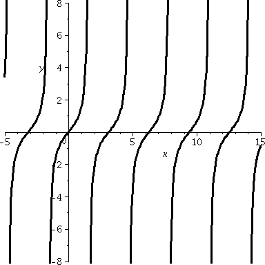 So the derivative of tan(x) is (sec(x))2, slightly
absurd. But Is this correct? Checking absurd things,
even a little bit, might be a good idea. Well, to the right is part of
the graph of tangent, which I hope you recognize. Look: in any
interval in which tangent is defined, the curves tilt "up" (more
properly, tan(x) is increasing in such intervals). Since
tan´(x) is supposed to be (sec(x))2 and sec(x) is
never 0 and squares are always positive, this means that slopes of
tangent lines to y=tan(x) will always tilt up. So we get some
confirmation of the slightly absurd fact.
So the derivative of tan(x) is (sec(x))2, slightly
absurd. But Is this correct? Checking absurd things,
even a little bit, might be a good idea. Well, to the right is part of
the graph of tangent, which I hope you recognize. Look: in any
interval in which tangent is defined, the curves tilt "up" (more
properly, tan(x) is increasing in such intervals). Since
tan´(x) is supposed to be (sec(x))2 and sec(x) is
never 0 and squares are always positive, this means that slopes of
tangent lines to y=tan(x) will always tilt up. So we get some
confirmation of the slightly absurd fact.
The parentheses are your pals
I tend to use lots and lots of parentheses when I compute derivatives
because otherwise I get confused. I also tend to be a bit
overcautious, perhaps. I always write "cosine squared" as (cos(x))2 and
not as cos2(x) because when I am a hurry and sloppy,
cos2(x) sometimes changes (all by itself?) into
cos(2x) or even cos(x2), both of which are, of course, very
different.
Composition and domain and range
We then took a digression from CALCULUS
and discussed what is probably officially a precalculus topic, and
which I think can be much more difficult than learning how to write
the derivatives of formulas: the
behavior of domain and range when functions are composed. I wrote
this as an independent web page but decided to take some class time
since some of the ideas are relevant to the next topic.
The next topic
we will learn about the Chain Rule, which is probably the most
important of the differentiation "rules". The Chain Rule describes how
to differentiate the composition of two functions each of whose
derivative is already known.
The Chain Rule
Suppose that f and g are differentiable functions. The
F(x)=fog(x)=f(g(x)) is differentiable, and
F´(x)=f´(g(x))·g´(x).
Here o is supposed to be a little circle, and the little circle
indicates composition. I will more frequently write F(x)=f(g(x)).
Suppose we are trying to analyze how a function, F, behaves under
perturbation (change, or kicking) of the input variable. We could
input x and get the output F(x). If we change the input variable by a
small amount, h, to a new value, x+h, the new output is F(x+h). This
might be complicated and difficult to understand. But if F is
differentiable, there's a nice description of the output: it is
F(x)+F´(x)h+(ErrF)h, where we have the old output,
F(x), and a change which is "linear" or first order, that is,
something (the derivative) multiplying the kick, and then
"higher order terms" (H.O.T.) which may be complicated, but as
h→0 much go to 0 faster than just constant multiples of h
alone. Probably in real physical situations with small changes, the
output changes would essentially be a multiplier of h because the
H.O.T. would generally be difficult to observe.
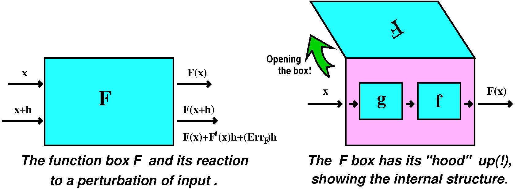
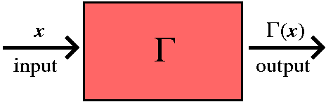
Now consider just a "function box", F, and attempts to
"experimentally" observe or evaluate the derivative. The situation
could be diagrammed as shown above. But it could be possible to lift
the lid (?) and look inside the F function box. It might be "wired" as
shown, with the input to F first going to an internal function box, g,
and then that output going to an internal function box, f. We will try
to analyze how changes to the input propagate or are transmitted
through this simple network. And maybe knowing things about f and g
will help us learn about f.
Consider the following complicated diagram, please:
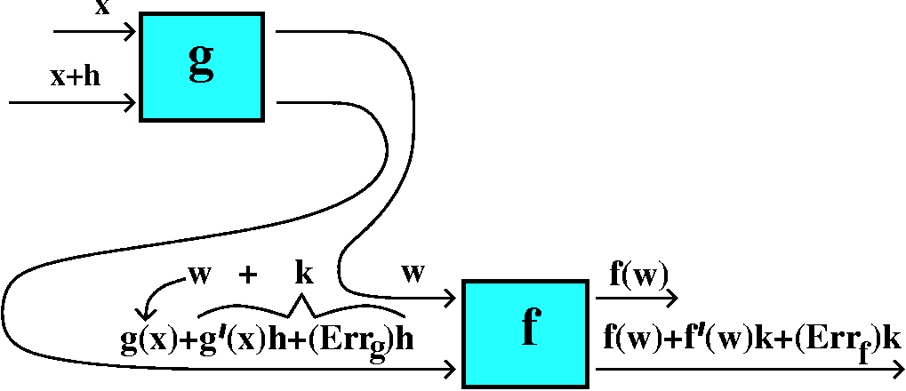
Function diagrams
I tried to make a supporting argument for the Chain Rule using
function diagrams. You can read the text for a more standard
discussion. If x is the input to a differentiable function, g, then
the output is g(x). If we perturb or change the input to g a bit, the
output, g(x+h), can be thought of in several parts:
g(x)+g´(x)h+(Errg)h. Here g(x) is the old output,
g´(x)h is a change in output which is directly proportional to h,
and there's other, higher order stuff, which→0 faster than h, so
Errg→0 as h→0.
Now we could take another differentiable function, f, with input w and
input perturbation k. The output will be f(w+k), and this can be imagined
it as f(w)+f´(w)k+(Errf)k. If we wire up the output of
g to the input of f, then we can try to think this way:
x+h→ g(x)+g´(x)h+(Errg)h
        w  \___________/
    THIS IS k WHEN CONSIDERING f's INPUT
          w   +   k  →  f(w)   +  f´(w)k     +  (Errf)k
                       f(g(x)) + f´(g(x))g´(x)h  +  (STUFF)h
Now the STUFF
turns out to be
f´(w)(Errg)+(Errf)g´(x)+(Errg)(Errf),
a whole bunch of things you don't need to remember but all of
which→0. So (STUFF)h is
H.O.T. ("Higher Order Terms" as I called them in class).
This means that the only first order term that comes out of g followed
by f is the change, h, multiplied by f´(g(x))g´(x).
This "multiplier" is exactly what characterizes F´(x).
The amplification factors multiply, but you need to evaluate them at
the correct values of their "arguments". This is the Chain Rule.
Basement example #1
If F(x)=(x2+7)300, what will F´(x) be? I
don't need the Chain Rule, not really (?), to compute
F´(x) because, after all, F(x) is "just" a polynomial (although
F(x) is a polynomial of degree 600, and this polynomial is not
presented in standard fashion). Success (rapid, accurate computation)
here probably will result from recognizing that the Chain Rule
applies.
If F(x)=f(g(x)), then g(x) is x2+7 so
g´(x)=2x, and f(x) is x300 so
f´(x)=300x299. Thus
F´(x)=f´(g(x))g´(x)=f´(x2+7)(2x)=300(x2+7)299(2x).
Whew!
How does a machine handle this?
Indeed, when asked to differentiate (x2+7)300,
Maple does recognize the composition and
uses the Chain Rule. This takes less than .001 seconds (timing is only
good up to a thousandth of a second). It is possible to force (!)
Maple to e-x-p-a-n-d this. That takes
.004 seconds, and then differentiation of that formula takes .002
seconds. This is a lot more time!
What people do in practice
But now comes the realistic comment. Hardly ever does anyone bother
writing down all of these intermediate steps. That is, in practice
very few f's and g's are actually identified. What happens is that
people see and differentiate the outside most function (f above), put
in the inner function (g) in that derivative, and then multiply by
g´. For example, consider sin(ex+x2). What
is its derivative? The outside function is sine, whose derivative is
cosine. So I begin writing cos(what's inside)·(the
derivative of what's inside). The result is
cos(ex+x2)·(ex+2x). This
expression is a formula for the derivative of
sin(ex+x2). Again, I urge you to consider the
significance and necessity (!) of appropriate parentheses in
these expressions. The "argument" of cosine is
ex+x2 and the cosine expression is then
multiplied by the expression (ex+2x).
#2
I think I found the derivative of sin(x2), a function which
occurs in the diffusion of light through things like plastic. Here the
outside function is sine and the inside function is x2. The
derivatie is cos(x2)(2x). There is a great deal of copying
when computing derivatives.
#3
I think I did another example, something like computing the derivative
of F(x)=e5x2+7sqrt(sin(x)). The outside most
function is "e-to-the-" (?) whose derivative is "e-to-the-". Therefore the
derivative, F´(x), will begin with
e5x2+7sqrt(sin(x)) and continue by multiplying
by the derivative of 5x2+7sqrt(sin(x)).
That's a sum, so its derivative is 10x+7·(the derivative of
sqrt(sin(x)). What's the derivative of sqrt(sin(x))? That itself is a
composition, with the "outside" function sqrt or
thing-raised-to-the-half-power. The outside derivative is
(1/2)(thing-raised-to-the-minus-half-power). So the derivative of
sqrt(sin(x)) is (1/2)(sin(x))–1/2(cos(x)). Now put it all
together:
if F(x)=e5x2+7sqrt(sin(x)) then
F´(x)=(e5x2+7sqrt(sin(x)))(10x+7((1/2)(sin(x))–1/2)).
I strongly recommend that you use lots of parentheses when
applying the Chain Rule.
| Function | Derivative |
|---|
| f(x) |
limh→0[f(x+h)-f(x)]/h |
|---|
| xn | nxn–1 |
|---|
| CONSTANT | 0 |
|---|
| ex | ex |
|---|
| f(x)+g(x) | f´(x)+g´(x) |
|---|
| f(x)·g(x) | f´(x)·g(x)+f(x)·g´(x) |
|---|
| CONSTANT(f(x)) | CONSTANT(f´(x)) |
|---|
| 1/f(x) | –f´(x)/[f(x)]2 |
|---|
| f(x)/g(x) |
[f´(x)g(x)–g´(x)f(x)]/[g(x)]2 |
|---|
| sin(x) | cos(x) |
|---|
| cos(x) | –sin(x) |
|---|
| cos(x) | –sin(x) |
|---|
| tan(x) | (sec(x))2 |
|---|
| sec(x) | sec(x)tan(x) |
|---|
| f(g(x)) | f´(g(x))·g´(x) |
|---|
In mathematics you don't understand things.
You just get used to
them. |
|---|
There will be a few more minor
entries to the table, but we are just about
done.
 QotD
QotD
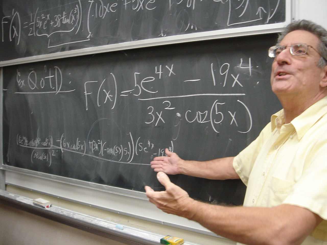
I wrote an entirely absurd formula defining a function and asked
people to write the derivative. To the right is a picture taken by
Mr. Lin (thank you!) slightly after the
event which contains the formula defining f(x). The person seen is
certainly older and heavier than I imagine myself, and he just looks
weird, as if he were preaching to a community of penguins. Or
something.
It may help you to know that I wrote the answer on the board as "you"
were working on it. Soon after, a student (whose name is unknown to me
but I would like to thank him) came up and looked at what I wrote. He
very calmly pointed out a mistake which I then fixed. Sigh: I
never make mistakes except fairly often.
Here is the question, and here is its solution, as done by my silicon pal, Si:
> time();
                                         0.003

> f:=(5*exp(4*x)-19*x^4)/(3*x^2*cos(5*x));
                                                        4
                                       5 exp(4 x) - 19 x
                              f := 1/3 ------------------
                                           2
                                          x  cos(5 x)

> time();
                                         0.005

> diff(f,x);
                        3                        4                         4
      20 exp(4 x) - 76 x        5 exp(4 x) - 19 x        (5 exp(4 x) - 19 x ) sin(5 x)
  1/3 ------------------- - 2/3 ------------------ + 5/3 -----------------------------
            2                        3                             2         2
          x  cos(5 x)              x  cos(5 x)                   x   cos(5 x)

> time();
                                         0.005
The machine was first told what f was and learned it in about .002
seconds. This "learning" takes a relatively long time (.002 is
lots of time) because the machine does not just remember the string of
symbols. It actually stores the formula as a logical pattern implied
by the various relationships, including arithmetic (addition,
multiplication, etc.) and composition. This is so that when requests
to do things (differentiation is only one "thing" that can be
requested) are received, the known logical structure will be used in
getting answers. The time required to differentiate took less than
.001 seconds! (The time command does not show increments of less than
one-thousandth of a second.) Different "invocations" of the program do
take different amounts of time, however, even for identical
computations. The program is very large, and when it is started, it
may be stored in different chunks of memory in various ways, and this
can increase the running time for some computations. But this is a
straightforward machine computation. I do not know why the
derivative is shown in what is, to me, a rather peculiar way. After
some irritating algebra, what is shown above is exactly the same as my
(corrected!) answer in the picture.
|
Here is the answer as done by
"hand" calculation:
(5e4x(4)–19·4x3)(x2cos(5x))–(5e4x–19x4)(3·2x·cos(5x)+3x2(–sin(5x)(5)))
---------------------------------------------------------------------
                             (x2cos(5x))2
People had to realize that the derivative of e4x is
(e4x)4, because this is also a use of the Chain Rule. The
outside function is "e-to-the-" and the inside function is
multiplication by 4.
Similarly, the derivative of cos(5x) is (–sin(5x))5: the outside
function is cosine and the inside function is multiplication by 5.
The use of lots of parentheses is a good thing here, because
then things become easier and less equivocal (uncertain) to read.
| Tuesday,
September 29 | (Lecture #8) |
|---|
The first exam in this course will be given on Thursday, October 8. A
great deal of review material is here. Please look at it.
Student "commitment"
I remarked that this course is a 5 credit course. This is a big chunk of credit. I remarked further:
- I had said near the start of the course that this course would
need a larger than usual commitment of time and energy from
students. In recent conversations I found that this "qualitative"
recommendation was misunderstood by people.
- More specifically and quantitatively, I think that YOU should study calculus about 2 hours every
evening. You should start this today. Certainly you may
consider this exaggerated, but Mr. Nakamura and myself are putting in
more than usual effort in our instruction, and I feel both you need to
do this also and you need to recognize the "weight" of 5
credits. You can recreate yourself -- you are not in
high school now, and you can decide to be a different person. Please
be a person who substantially pushes towards success. Yes,
intelligence and talent (and luck!) matter, but persistence is essential to
success. Please work with other students
in the course.
What's the range?
Here's a function: f(x)=(1x+2)/(3x2+4). Since
3x2+4 is always at least 4, the bottom is never 0. The
domain of this function is all real numbers. So the collection of
inputs is all numbers. What can we say about the collection of
all possible outputs, the range of this function? I claim this
is not totally clear.
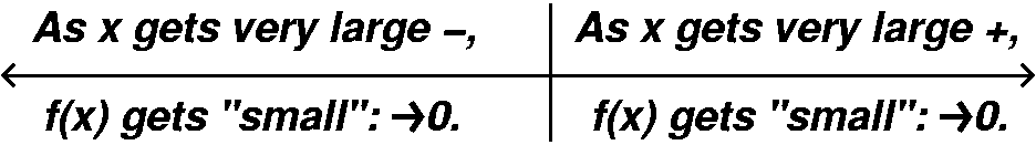
Certainly, if x is very very large positive, the fraction
=(1x+2)/(3x2+4) will become small. (The limit as
x→+∞ of f(x) is 0, we will later say.) A similar thing is
true as x→–∞. Both of these limits or asymptotic
behaviors or whatever you want to say occur because the bottom is a
degree 2 polynomial, and the top is a degree 1 polynomial, and the
high degree polynomial "dominates". I'll be more precise about this in
the future. We learned a bit about f when I asked people to give me
approximate graphs using their calculators. Also, notice that f(–2)=0
and that's the only x-intercept (crossing of the horizontal
axis) for this function.
But what happens in between? What sorts of numbers can we get out of
f? Well, f(1)=3/7, so 3/7 is in the range. And f(2)=4/16=1/4, so 1/4
(sigh!) is in the range. And ... and ... I think just listing numbers
is not even simple fun, and is mostly pointless. One nice suggestion
for an output, though, was 0. The only x which gives 0 is
–2. (Why? Well, Top/Bottom is 0 exactly when Top=0 [think about
it] and this is 1x+2=0.) This is good because now I know that the only
sign change is at –2, and (Intermediate Value Theorem) this is
where f's outputs change from positive to negative or negative to
positive.
How can we systematically learn about f? Well, I do know (Quotient
Rule) that
f´(x)=[(1)(3x2+4)–(1x+2)(6x)]/(3x2+4)2.
When can this be 0? Only when the top is 0, so let me "simplify" the
top:
(1)(3x2+4)–(1x+2)(6x)=3x2+4–6x2–12x=–3x2–12x+4.
So the top is 0 when –3x2–12x+4=0. We need to
use the quadratic formula (hey, very few "random" degree 2 polynomials
with integer coefficients actually can be written as a product of two
degree 1 polynomials with integer coefficients so simple-minded
factoring generally won't work!). The roots are
–2–(4/3)sqrt(3) and –2+(4/3)sqrt(3). (I wrote
something much more horrible in class, and this is what results after
some arithmetic.) You can check (as I did in class) that these roots
are at least approximately numerically correct and consistent with the
graph as the x-coordinates of the "bumps".
What do I know about the SIGN of f´? This derivative is a
quotient, and the bottom is (3x2+4)2. The bottom
is always positive. So the SIGN of f´ in this case is determined
by the sign of the top. But the top is –3x2–12x+4. This is
a parabola, and because the coefficient of x2 is –3<0,
the parabola opens down. From this and from knowing the two
roots of the top, we see:
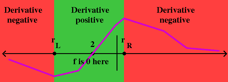
- If x<–2–(4/3)sqrt(3) then f´(x)<0.
- If –2–(4/3)sqrt(3)<x<–2+(4/3)sqrt(3) then f´(x)>0.
- If x>–2+(4/3)sqrt(3) then f´(x)<0.
So there seems to be quite good information about f. We will go over
things like this is great detail later in the course -- this is a
first attempt to show how knowing even just a little bit is enough to
answer an irritating question. In the graph to the right,
rL is the left-hand root of f´(x)=0: it is
–2–(4/3)sqrt(3). rR is the right-hand root:
–2+(4/3)sqrt(3).
So what will the range of f be, exactly? It seems "clear" looking even
at the approximate graph shown to the right that the range will be all
numbers between f's values at rL and rR.
 That
is, the range is the interval [f(rL),f(rR)]. I can be
more precise, of course. The range is
[f(–2–(4/3)sqrt(3)),f(–2+(4/3)sqrt(3))], and this is (after some work
which I would not inflict on people in class!)
[(1/4)–(1/6)sqrt(3),(1/4)+(1/6)sqrt(3)].
That
is, the range is the interval [f(rL),f(rR)]. I can be
more precise, of course. The range is
[f(–2–(4/3)sqrt(3)),f(–2+(4/3)sqrt(3))], and this is (after some work
which I would not inflict on people in class!)
[(1/4)–(1/6)sqrt(3),(1/4)+(1/6)sqrt(3)].
What this is, and what this is not
I do not claim that the computations just done are wonderful. Maybe
they are not even interesting. But if you absolutely need to know the
answer to questions of that type, and you need to know with great
accuracy, and great certainty, then the analysis we've done is
probably the best way. It really allows us to get the correct numbers,
and the procedure is understandable. It is also inherently more
precise than using a graphing device, although I probably would try to
get an approximate answer using a graph first.
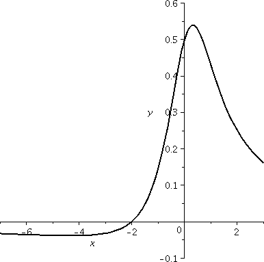
By the way, to the right is, of course, a graph (in a weird window,
check the axes!) of y=f(x). I hope you can "see" the
range. Incidentally,
[(1/4)–(1/6)sqrt(3),(1/4)+(1/6)sqrt(3)] is approximately
[–0.039,0.539].
Building a BIG cylinder inside a sphere
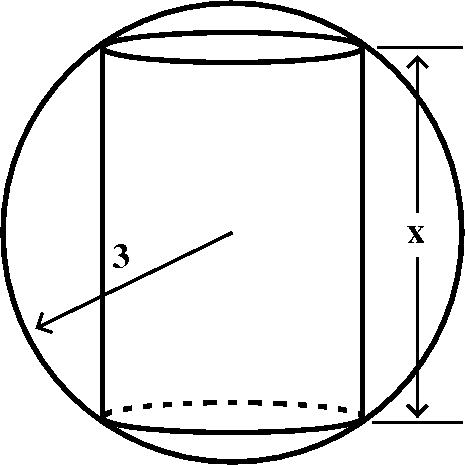 One of the recent workshop problems asked students to analyze the
problem of a cylinder "inscribed" inside a sphere. So the cylinder
touches the sphere as mucl as possible. The task is to understand how
to write a formula for the volume of the cylinder as a function of the
cylinder height, and to also tell what the domain of that formula is,
considering the origin of the problem. Here we will look at the
formula obtained when the radius of the sphere is 3.
One of the recent workshop problems asked students to analyze the
problem of a cylinder "inscribed" inside a sphere. So the cylinder
touches the sphere as mucl as possible. The task is to understand how
to write a formula for the volume of the cylinder as a function of the
cylinder height, and to also tell what the domain of that formula is,
considering the origin of the problem. Here we will look at the
formula obtained when the radius of the sphere is 3. 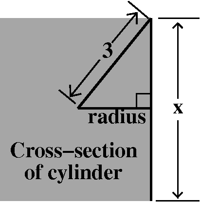 The height of the cylinder is related to the cylinder's
radius using Pythagoras, if we look at a cross-section of the
cylinder. If x is the height of the cylinder, then
V(x)=Π(9–x2/4)x. The domain of V(x), when
considering this problem, is 0<x<6 or 0≤x≤6. It is almost
one's own personal philosophy determines whether cylinders with
dimensions and volume equal to 0 should be included in this
analysis. I don't think a cylinder can have a negative height, and I
don't think a cylinder insider a sphere of radius 3 can have a height
bigger than the diameter of the sphere, which is 6.
The height of the cylinder is related to the cylinder's
radius using Pythagoras, if we look at a cross-section of the
cylinder. If x is the height of the cylinder, then
V(x)=Π(9–x2/4)x. The domain of V(x), when
considering this problem, is 0<x<6 or 0≤x≤6. It is almost
one's own personal philosophy determines whether cylinders with
dimensions and volume equal to 0 should be included in this
analysis. I don't think a cylinder can have a negative height, and I
don't think a cylinder insider a sphere of radius 3 can have a height
bigger than the diameter of the sphere, which is 6.
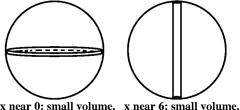
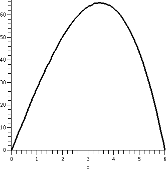 We can
graph V as a function of the height, x. When x is close to 0, the
cylinder is short and wide, but the shortness (a factor of x) makes
V(x) quite small. When x is near 6, the cylinder is tall, but the
radius is very small (36/4 is 9!) so the V(x) is also quite small.
We can
graph V as a function of the height, x. When x is close to 0, the
cylinder is short and wide, but the shortness (a factor of x) makes
V(x) quite small. When x is near 6, the cylinder is tall, but the
radius is very small (36/4 is 9!) so the V(x) is also quite small.
 How can we find the cylinder of largest volume inside this sphere?
That will be at the "top" of the graph, and I will locate the top by
compute V´(x). So this is (Product Rule)
Π(–2x/4)x+Π(9–x2/4). This will be 0 when (divide by Π,
collect x2's): 9–(3/4)x2=0, so x=2sqrt(3) (the
negative root is not in the domain for this problem!). Indeed, if you
look at the graph, the top of the graph seems to be at about 3.4. This
specifies the cylinder. The radius and the volume can then be
computed.
How can we find the cylinder of largest volume inside this sphere?
That will be at the "top" of the graph, and I will locate the top by
compute V´(x). So this is (Product Rule)
Π(–2x/4)x+Π(9–x2/4). This will be 0 when (divide by Π,
collect x2's): 9–(3/4)x2=0, so x=2sqrt(3) (the
negative root is not in the domain for this problem!). Indeed, if you
look at the graph, the top of the graph seems to be at about 3.4. This
specifies the cylinder. The radius and the volume can then be
computed.
What this is, and what this is not
Again: this is not a profound problem! But it does show a
systematic way to solving such problems. There may be computational
details which can be irritating, but at least we have some method to
work with. And I assure you that we will go into great detail about
the general method later in this course.
We move on to lengthen the list of derivatives by a few more entries.
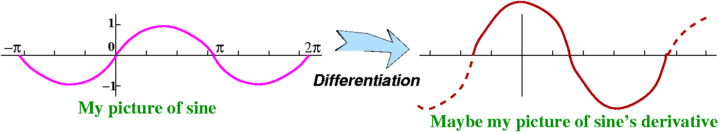
The derivative of sine: a guess
I began by (trying to) draw an accurate picture of sine and then
discussing the slopes of the tangent lines to this curve. The derivative of sine, is, of course, exactly those slopes.
Where would the derivative of sine be 0? Well, where the
tangent lines are horizontal. That should be at the tops and bottoms
of the sine curve. These occur at Π/2, 3Π/2, –Π/2, etc.: lots of
places because sine repeats every 2Π.
Let's look at sine between, say, x=–Π/2 and x=Π/2. The derivative,
the slope of the tangent line, would start out at –Π/2 at 0, then it
would increase (as the tangent line began to tilt up). Then it would
tilt up more (the slope would be more positive) until it would begin
to tilt "down": here the language gets complicated. I am not asserting
that the derivative is negative, but I am merely asserting that the
slope, which stays positive, begins to decrease. Eventually the slope
becomes 0 again when x=Π/2.
What should happen between x=Π/2 and x=3Π/2? In that interval the
sine curve is sort of a downwards reflection of the behavior in the
interval [–Π/2,Π/2]. The derivative starts at 0, then becomes
negative. It gets more negative, then gets less negative, and ends up
at 0. The shape of the derivative exactly reflect the shape in the
earlier interval, since the sine curve's shape is a flip of the
earlier behavior.
The derivative repeats every 2Π, since y=sin(x) repeats every 2Π. I
drew sort of what is shown below. The derivative of sine qualitatively
looks like cosine, except maybe we don't know the scaling factor: how
high the curve is. Things are wonderful: the scaling factor is 1.
The derivative of sine: via limits, algebra, etc.
In a calculus textbook, something like the following is done when
f(x)=sin(x):
 sin(x+h)–sin(x)     sin(x)cos(h)+sin(h)cos(x)–sin(x)
----------------- = ---------------------------------- = PIECE #1 + PIECE #2
        h                          h
where
                   sin(h)
PIECE #1 = cos(x) --------
                     h
and as h→0 this → cos(x)·1 because we arranged it this
way when we decided to use radian measure! Also,
                   cos(h)–1
PIECE #2 = sin(x) ----------
                       h
If we multiply this top and bottom by cos(h)+1, the result on top is
[cos(h)]2–1 which is [sin(h)]2. Then
                    [sin(h)]2             sin(h)               1
PIECE #2 = sin(x) ------------- = sin(x) -------- sin(h) ------------
                   h [cos(h)+1]             h             [cos(h)+1]
Now as h→0, I claim:
               sin(h)                     1
sin(x)→sin(x); ------ →1;  sin(h)→0; ----------- → 1/2.
Nothing happens!      h                    cos(h)+1
So the result is sin(x)·1·0·1/2=0.
The two pieces work out exactly so that the derivative of sine is
cos(x)·1+sin(x)·0, just we want and would have hoped.
I believe this is the only time in the course I'll
even write the addition formula for sine.
What's up with degrees?
If you insist on using degrees in your calculus computations,
well, things are different and really not so nice. I suggest, please,
that you put your calculator in degree mode, and that you then graph
sin(h)/h for h near 0. That is, try to see graphically what the limit
of sin(h)/h as h→0 is. Well, if you do this (and I recommend it
if you are "allergic" to radians) you will find out that
limh→0sin(in degrees)(h)/h≈0.01745329252
(heh, heh, approximately). This means that, in degrees, the
derivative of sine will be about .017453 multiplied by cosine. Well,
no one in the world wants to work with such numbers floating
around. They are ugly and complicate many computations. Yes, the Good
Lord may have made the world, but human beings can fuss with things to
have the details a bit more nice. One of the nice details is measuring
angles in radians, so the derivatives of trig functions are
simpler. (This is the same sort of reason that e is chosen as the base
of the standard exponential function -- to make the derivative of
"the" exponential function simpler.)
|
The derivative of cosine
Look again at the shape of the graphs drawn just above. If I move the
coordinate axes Π/2 to the right, the graph of sine becomes the graph
of cosine. The candidate graph for the derivative needs to be
recognized. It is actually minus the graph of sine. This minus
sign is slightly annoying, and sometimes I screw up and forget it or I
put it where it shouldn't be. The derivative of cos(x) is
&ndashsin(x). (There is a shift of Π/2 in both graphs.)
More trig functions?
There are 6 trig functions. The most important are certainly sine and
cosine, and then tangent. Sometimes useful is secant. I will find the
derivatives of tangent and secant on Thursday. I will also then put in
another line, the most important one, in the derivative table. So far
we have what follows.
| Function | Derivative |
|---|
| xn | nxn–1 |
|---|
| CONSTANT | 0 |
|---|
| ex | ex |
|---|
| f(x)+g(x) | f´(x)+g´(x) |
|---|
| f(x)·g(x) | f´(x)·g(x)+f(x)·g´(x) |
|---|
| CONSTANT(f(x)) | CONSTANT(f´(x)) |
|---|
| 1/f(x) | –f´(x)/[f(x)]2 |
|---|
| f(x)/g(x) |
[f´(x)g(x)–g´(x)f(x)]/[g(x)]2 |
|---|
| sin(x) | cos(x) |
|---|
| cos(x) | –sin(x) |
|---|
In mathematics you don't understand things.
You just get used to
them. |
|---|
QotD
Here is the question, and here is its solution, as done by my silicon pal, Si:
> time();
                                                0.002

> f:=(3*x+exp(x)+7*sin(x))/(x^2+5*cos(x));
                                          3 x + exp(x) + 7 sin(x)
                                     f := -----------------------
                                                2
                                               x  + 5 cos(x)

> time();
                                                0.002

> diff(f,x);
                                   3 + exp(x) + 7 cos(x)   (3 x + exp(x) + 7 sin(x)) (2 x - 5 sin(x))
                                   --------------------- - ------------------------------------------
                                        2                                   2            2
                                       x  + 5 cos(x)                      (x  + 5 cos(x))
> time();
                                                0.002
The time required took less than .001 seconds because the time command
does not show increments of less than one-thousandth of a
second. Sigh. Different "invocations" of the program do take different
amounts of time, however, even for identical computations. The program
is very large, and when it is started, it may be stored in different
chunks of memory in various ways, and this can increase the running
time for some computations. But this is a straightforward machine
computation.
| Thursday,
September 24 | (Lecture #7) |
|---|
I made several comments. First, what is the derivative? Well,
here, again:
A function f is differentiable at x if
the limit limh→0[f(x+h)–f(x)]/h exists. When that
limit exists, then its value is called the
derivative of f at x, f´(x).
There are many interpretations of the derivative. This is
certainly the principal reason people learn about it. For example, it
is the slope of a line tangent to the graph, y=f(x). Or, if f(x)
represents the position of a point at time x, then f´(x) is the
(instantaneous) velocity of the point at that time. Many other
meanings can be given to derivatives, and using them will allow us to
solve fairly easily a large number of otherwise difficult problems.
Then I discussed the economics of hiring an engineer. A few years ago
I looked up generally available labor information. The annual cost of
hiring a new mechanical engineer, with a first college degree (a
bachelor's degree) with no previous professional experience, in the
NY/NJ metropolitan area, was way above $100,000. Please note that this
is the cost to the employing firm, so it is not just the salary. I
wanted to contrast this with the fact that there are free
computer programs which will take functions defined by formulas
involving familiar functions and produce a formula for the derivative
of that function. Therefore, computing derivatives of formulas can't
be what people want since that's easy. What's wanted is the
ability to model and investigate complicated situations, and
understand how to apply appropriate technical tools. At the calc 1
level, that is what this course is about. Yes, you will need to learn
to take a formula and produce a derivative, but that's only the
beginning.
QotD
Find the derivative of f(x)=sqrt(x) from the definition of
derivative.
My silicon friend and Γ
 There is an important function called the Gamma function and
its value at x is usually written Γ(x). I am not
inventing this function. There are over 1,000,000 references to it on
Google. I wanted to use this function to force people to think
about derivatives. I chose this specific function because I thought
that students were unlikely to be familiar with it, and also because
their calculators would likely not be able to compute it
easily. Γ is a function which students are unlikely to "meet"
until junior and senior level courses. My silicon friend, my rather
new laptop, can compute values of this function, and do arithmetic on
these values. So all that was known is that Γ was a mysterious
"box" (shown to the right!) which could be investigated with
experiments. I told students I would be willing to use it to answer
questions such as Γ(3)=2 and Γ(4.7)=15.43141. Students
were bewildered, especially when I asked these questions:
There is an important function called the Gamma function and
its value at x is usually written Γ(x). I am not
inventing this function. There are over 1,000,000 references to it on
Google. I wanted to use this function to force people to think
about derivatives. I chose this specific function because I thought
that students were unlikely to be familiar with it, and also because
their calculators would likely not be able to compute it
easily. Γ is a function which students are unlikely to "meet"
until junior and senior level courses. My silicon friend, my rather
new laptop, can compute values of this function, and do arithmetic on
these values. So all that was known is that Γ was a mysterious
"box" (shown to the right!) which could be investigated with
experiments. I told students I would be willing to use it to answer
questions such as Γ(3)=2 and Γ(4.7)=15.43141. Students
were bewildered, especially when I asked these questions:
Is Γ(x) differentiable at x=3? Give some evidence supporting
your assertions. If the answer is
yes, what is an approximate value of for Γ´(3)?
These are emphatically sophisticated questions. Answering them
needs some thinking. We had quite a discussion, which took much more
time than I expected but which may have been helpful, I hope! Thinking
that Γ´(3) is the slope of a tangent line to a graph
probably doesn't help with answering this question.
First I was asked to compute some values of Γ and I asked how
this helped. I directed people's attention to the definition and asked
how we could use that definition to possibly answer the
questions. Well, fairly soon people asked me to compute some rather
strange quotients, and with the computer I was able to respond:
- [Γ(3+.001)–Γ(3)]/(.001)=1.84682 (approximately!)
- [Γ(3+.0001)–Γ(3)]/(.0001)=1.84569 (approximately!)
- [Γ(3–.0001)–Γ(3)]/(–.0001)=1.84544 (approximately!)
I liked this suggestion very much because it
shows a slightly and appropriately suspicious nature: the limit is
supposed to be two-sided, so let's check a little bit that things
do seem to work correctly.
- [Γ(3+.00001)–Γ(3)]/(.00001)=1.84558 (approximately!)
Students then decided enough information was present to answer the
questions. So: YES, Γ is
differentiable at x=3. The computations shown above give evidence
supporting this assertion, because for some "small" numbers, the
difference quotient computed seems to get close to about 1.8455 or
so. Therefore this would also be an approximate value for the
derivative. I was sort of happy.
 More about this silly question
Since the darn function is actually quite useful, much more is known
about it than I presented. A wikipedia article is here and a
Gamma function calculator is here (on a
web page created by a group interested [really!] in "Engineering
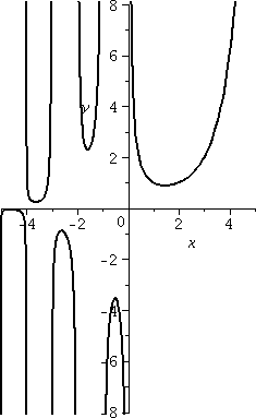
Fundamentals"). A graph of y=Γ(x) for x between –5 and 5 is
shown to the right. I would say that graph is VERY strange,
very very strange.
 Here is maybe a little more support for the answers which were given
to the previous questions. I do like pictures (probably too
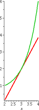
much!). My machine reports that Γ(3)=2. If the reported
derivative is correct, then 1.8455 should be the slope of the line
tangent to y=Γ(x) when x=3. This line should go through the
point (3,Γ(3)) which is (3,2). An equation for this tangent line
should be y–2=(1.8455)(x–3). The picture to the right shows (for x
between 2 and 4) both the curve y=Γ(x) in red and the candidate for the tangent line in green. The picture looks good to me.
Here is maybe a little more support for the answers which were given
to the previous questions. I do like pictures (probably too
much!). My machine reports that Γ(3)=2. If the reported
derivative is correct, then 1.8455 should be the slope of the line
tangent to y=Γ(x) when x=3. This line should go through the
point (3,Γ(3)) which is (3,2). An equation for this tangent line
should be y–2=(1.8455)(x–3). The picture to the right shows (for x
between 2 and 4) both the curve y=Γ(x) in red and the candidate for the tangent line in green. The picture looks good to me.
|
Our task beginning this week is building a table of derivatives. It
will turn out that for functions defined by familiar formulas, the
derivatives can be written "easily". The quotes around the word mean
that I hope you will be able to write something which looks like the
derivative for functions defined by formulas of reasonable size, and
that most of the time (97%?) you will be correct. I hope that you'll
also be able to look at the output of computer programs that are
supposed to find derivatives, and you'll have some feeling for what
the outputs should be. For example, if you ask a program for the
derivative of x17 and the output is arctan(x), maybe you'll
go, "Huh?" Here's what we have so far:
| Function | Derivative |
|---|
| xn | nxn–1 |
|---|
I actually proved this in the last lecture when n is a positive
integer. It is, in fact, true for any constant n. So examples
would be:
- x17 whose derivative is 17x16.
- sqrt(x), which you might see as x1/2, and its
derivative is (1/2)x–1/2, which can also be written as
1/(2sqrt(x)).
- 1/x9, which is x–9, and its derivative is
–9x–10, which can also be written as –9/x10.
Here's a comment about the different ways of writing exponents: I will
be happy with any correct notation that you use. You might
prefer (and we will prefer!) certain notation over others depending on
how we'll use results. But right now, all I want is some form of the
correct answer.
Constants
I want f´(x)=limh→0[f(x+h)–f(x)]/h. What if f is a
CONSTANT function, so its values are all the same?
Well then the top of the difference quotient, f(x+h)–f(x), will be
CONSTANT–CONSTANT, and it will be 0.
So the derivative will be 0.
| Function | Derivative |
|---|
| xn | nxn–1 |
|---|
| CONSTANT | 0 |
|---|
ex
Let's consider the derivative of an exponential function, say
ax, where a is a constant. Then the difference quotient,
[f(x+h)–f(x)]/h becomes [ax+h–ax]/h. As I
mentioned in class, just plugging in h=0 yields 0/0, and this doesn't
help. We can try the algebra that's available:
[ax+h–ax]/h=[axah–ax]/h=ax((ah–1)/h).
So we need to consider (ah–1)/h as h→0.
We actually analyzed this limit graphically and numerically in Lecture
#3 for several values of a. When a=2, it seems that the limit exists
and equals .693, while if a=3, 1.109 was the approximate value of the
limit. Since f´(x) will be equal to ax
multiplied by whatever the value of
limh→0(ah–1)/h is, I want to choose a value of
a so that the formulas are as simple as possible. So maybe we can get
a value of a so the limit of (ah–1)/h as h→0 is 1.
This can be done. In fact, here is a fairly irritating way of
thinking about this special number, which people call e. If h is
small,
we would like (ah–1)/h to be approximately 1 when h is
small, well, look at the following sequence of ideas:
| n | (1+{1/n})n |
|---|
| 1 | 2.000000000 |
| 2 | 2.250000000 |
| 3 | 2.370370369 |
| 4 | 2.441406250 |
| 5 | 2.488320000 |
| 10 | 2.593742460 |
| 100 | 2.704813829 |
| 1,000 | 2.716923932 |
| 10,000 | 2.718145926 |
| 100,000 | 2.718268237 |
| 1,000,000 | 2.718280469 |
-
Since
(e1/100–1)/{1/100} should be approximately 1 we
could multiply by 1/100 and see that
(e1/100–1) is approximately 1/100.
- Now add 1 to both sides and see that
e1/100 is approximately 1+{1/100}.
- If we took the 100th power (raised things to the 100)
then the 1/100 and 100 in the exponent of e cancel (repeated
exponentiations multiply) so that
e is about (1+{1/100})100.
Well, the numerical value of (1+{1/100})100 about
2.704813829. To the right is a table of values of
(1+{1/n})n. This method of "computing" or approximating e
is actually very very slow. ere are
several million digits of e, if you need them. As I mentioned
in class, it is certainly possible to prove that the formula converges as n gets
large. This can be done with "only" high school algebra. It is quite
tedious, and, to me at least, has little redeeming social value. (I
may have the wrong attitude here, so please forgive me.)
| Function | Derivative |
|---|
| xn | nxn–1 |
|---|
| CONSTANT | 0 |
|---|
| ex | ex |
|---|
What does that limit statement mean?
The definition f´(x)=limh→0[f(x+h)–f(x)]/h is
sometimes a bit difficult to understand. What if I just throw out
"limh→0"? Well, certainly f´(x) is NOT the same as [f(x+h)–f(x)]/h (hey: one of
them has an h and the other doesn't even mention h!). So it really
means f´(x)=[f(x+h)–f(x)]/h+ERR, where ERR (stands for "ERROR",
of course) is some "mess", and all I know about it (and care about it,
at this time!) is that it goes to 0 as h goes to 0. I don't like
division, so let me multiply by h. Here's the result:
f´(x)h=f(x+h)–f(x)+ERR·h.
I don't like subtraction, so let me add f(x).
f(x)+f´(x)h=f(x+h)+ERR·h.
People usually put the "ERR" term on the other side, so let me do
that. It is irritating, but I won't change the sign on the ERR term,
because right now I am interested in the qualitative aspect. So what I
have is:
So what the heck do we have? If we think of the function as taking an
input variable, x, and smooshing (?!) it around to get an output
value, f(x), then f(x+h) is what results if we "kick" the input value
by a little bit, h. If f is differentiable, then the output seems to
split up into several pieces.
- The old value, f(x). If h is very very very small, we should
expect to see only something that looks like f(x). This is continuity
-- there will be no big jumps if the input is changed just a little.
- Suppose h is small, but not (somehow!) very very very small. Then
we should see some change in the output. If f is differentiable, the
major change will be a CONSTANT multiplying the input change. The
multiplier is the value of the derivative.
- So the two terms before aren't all. There's also
"ERR·h". This is stuff that is much smaller than h. In reality,
I would not expect to observe this for small h. It is "higher order"
than h (people think of h3, for example: when h is small,
higher order stuff is much smaller).
Sums
Suppose f and g are differentiable functions. Then I know:
f(x+h)=f(x)+f´(x)h+Errf·h
g(x+h)=g(x)+g´(x)h+Errg·h
I used different notation for the error terms for f and g to keep track of stuff
better than I did in class.
I can add these equations. Here's the result:
f(x+h)+g(x+h)=f(x)+f´(x)h+Errf·h+g(x)+g´(x)h+Errg·h
but this is an awfully silly way to write the result. I should write
it in such a way that the "structure" of the equation is shown. Here:
(f(x+h)+g(x+h))=(f(x)+g(x))+(f´(x)+g´(x))h+([Errf+Errg]h)
The left-hand side is the function f+g at the input value x+h.
The first piece, (f(x)+g(x)), is the unperturbed value of the function f+g
at x. The second piece,
(f´(x)+g´(x))h, is a multiplier not involving h,
multiplied by h. The third piece is h multiplied by some stuff:
[Errf+Errg], and all this stuff→0 as
h→0. Hey, this is the higher order vanishing. So I know the next
line in the table.
| Function | Derivative |
|---|
| xn | nxn–1 |
|---|
| CONSTANT | 0 |
|---|
| ex | ex |
|---|
| f(x)+g(x) | f´(x)+g´(x) |
|---|
Products
This is harder and I will be a bit more detailed than what I did in a
hurry in class.
Suppose I know
f(x+h)=f(x)+f´(x)h+Errf·h
g(x+h)=g(x)+g´(x)h+Errg·h
and now I multiply the equations. Well, the left-hand side isn't
bad, but there are three terms on the right-hand side of each
equation, so there will be NINE terms if I distribute out the
product/sums. I am really considering the product function of f and
g. Here is how to organize the result. In class we thought a bit about
how to organize this. In "print" such discussion is more difficult to
write.
Please: I don't want all this stuff to be memorized. I haven't
memorized it. But I do know the general idea, and that's what I'd like
you to get used to. Here is the left-hand side:
(f(x+h)·g(x+h)). This
is the function f·g's value at x+h.
Here are the pieces of the product of the two
right-hand sides:
(f(x)·g(x)). This
is the function f·g's value at x: the "old", unperturbed value
of f·g.
(f´(x)·g(x)+f(x)·g´(x))h. This is the first-order term, stuff (no h's!)
multiplied by one h.
Here is all the rest of the stuff. There are (good
grief!) six different terms. But I can "pull out" one h from all of
these terms, and what is left in all six of these terms are things
that →0 as h→0. Wow!
(f(x)·Errg+f´(x)·g´(x)h+f´(x)·Errgh+f(x)·Errf+Errf·g´(x)+Errf·Errgh)h.
If you see this, sort of, then you can see the next line of the
table.
| Function | Derivative |
|---|
| xn | nxn–1 |
|---|
| CONSTANT | 0 |
|---|
| ex | ex |
|---|
| f(x)+g(x) | f´(x)+g´(x) |
|---|
| f(x)·g(x) | f´(x)·g(x)+f(x)·g´(x) |
|---|
A quote from von Neumann
John
von Neumann (1903-1957) was a mathematician who was raised in
Hungary and spent most of his career in the United States. He worked
in many areas of pure and applied mathematics. His ideas were
influential in quantum mechanics, the development of nuclear weapons,
game theory, and the theory and construction of digital computers.
In mathematics you don't understand things. You just get used to
them.
The last entry in the derivative table is frequently called "the
Product Rule". I think the Product Rule is one of those things you
need to "just get used to".
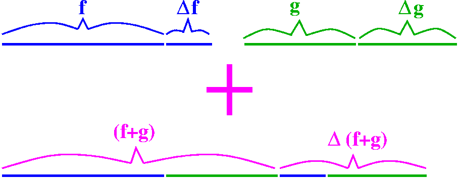 Another way of looking at products
Well, first let's reconsider addition. We could imagine f and g being
functions that somehow model intervals which are growing in length. At
a certain time, the intervals have some length (the lengths labeled
just f and g to the right). If we increase time ("+h") then each
interval grows. I used the Greek capital Delta ( ) to indicate how much
each would grow. If we combine the functions with addition, then the
growth just adds. To me this is sort of straightforward. I hope it is
to you. Since the growths add, the average growths add, and the
"instantaneous growths" (the derivatives!) also just add. ) to indicate how much
each would grow. If we combine the functions with addition, then the
growth just adds. To me this is sort of straightforward. I hope it is
to you. Since the growths add, the average growths add, and the
"instantaneous growths" (the derivatives!) also just add.
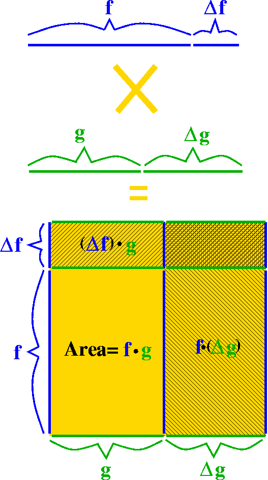 A
simple physical (?) model of multiplication in this setting would be
to just make the intervals into sides of a rectangle. Then the
area of the rectangle will be the product function,
f·g. When we allow the intervals to grow, the area grows in a
more complicated manner. Look at the picture: the increase of the area
has three "chunks". One of them is an increase in f multiplied by
g. Another is f, multiplied by the increase in g. Then there's the
corner piece, which is increase in f multiplied by increase in g. When
the increments get small, the corner piece's decrease is much faster
than the two other pieces' decreases. (Sorry: my use of language is
not very good here.) So I think that the instantaneous increase
in f·g will be given by f´(x)g(x)+f(x)g´(x): these
are the first order terms of the increase. Of course, this is the
product rule. A
simple physical (?) model of multiplication in this setting would be
to just make the intervals into sides of a rectangle. Then the
area of the rectangle will be the product function,
f·g. When we allow the intervals to grow, the area grows in a
more complicated manner. Look at the picture: the increase of the area
has three "chunks". One of them is an increase in f multiplied by
g. Another is f, multiplied by the increase in g. Then there's the
corner piece, which is increase in f multiplied by increase in g. When
the increments get small, the corner piece's decrease is much faster
than the two other pieces' decreases. (Sorry: my use of language is
not very good here.) So I think that the instantaneous increase
in f·g will be given by f´(x)g(x)+f(x)g´(x): these
are the first order terms of the increase. Of course, this is the
product rule.
Examples
The derivative of 37x88: well, this is a product. It is
37·x88. Here f(x)=37 and g(x)=x88. So
f´(x)g(x)+f(x)g´(x) becomes
0·x88+37·88x87. Most people think
that multiplication by a constant deserves an entry of its own. So
back to the table:
| Function | Derivative |
|---|
| xn | nxn–1 |
|---|
| CONSTANT | 0 |
|---|
| ex | ex |
|---|
| f(x)+g(x) | f´(x)+g´(x) |
|---|
| f(x)·g(x) | f´(x)·g(x)+f(x)·g´(x) |
|---|
| CONSTANT(f(x)) | CONSTANT(f´(x)) |
|---|
- 47x32+sqrt(Pi)x12–.007x2+99
has derivative
47·32x31+sqrt(Pi)·12x11–.007·2x+0.
So now we can differentiable polynomials. People who aren't as neat as
I am might leave out the +0. :-)
- 8ex–9x1/3 has derivative
8ex–9·(1/3)x–2/3.
- Consider
(5ex–9x)(x12–12/x3). This is a
product with f(x)=5ex–9x and
g(x)=x12–12/x3 (but also recognize that
–12/x3 is –12x–3). This has derivative
(5ex–9)(x12–12/x3)+(5ex–9x)(12x11–12(–3)/x4)
- Look at, say, x12. This can also be written
x7·x5. If we use the Product Rule, we
will get
7x6·x5+x7·5x4. If
we "clean up" a bit, we seem to get 7x6+5+5x7+4
which is 7x11+5x11 which is
12x11. That is the correct and expected answer, so the
weird Product Rule does reinforce what we already know.
|
| Tuesday,
September 22 | (Lecture #6) |
|---|
 Again: problem #5 in section 2.7
Here's the problem:
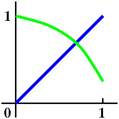
Show that cos(x)=x has a solution in the
interval [0,1].
Since I am a picture person, I frequently try to draw a graph or two
to understand what the problem is about. In this case, certainly the graph of y=x is easy to imagine on [0,1]. What
about y=cos(x)? Well, it does help, if you don't have access to a
graphing device, to know that cos(0)=1. I know that cosine drops down
as x increases from 0. What do we know about cos(1)? As one student
declared, cos(1) is both less than 1 and greater than 0. That's
because Π/2 is about 1.57 and cosine decreases between 0 and Pi/2,
and does not reach 0 until Π/2. So the graph of
y=cos(x) decreases from (0,1) to (1,cos(1)), and the end point
is somewhere above the x-axis. The mental picture I have built is
shown to the right. I deliberately did not have a graphing
device create an "accurate" display of the situation -- I wanted to
show what we should be able to do inside our own heads.
The picture now encourages me to believe the assertion of the
problem. The text supplies this hint:
Show that f(x)=x–cos(x) has a zero in
[0,1].
The phrase "has a zero in [0,1]" means that there is some root of
f(x)=0 in the interval [0,1]. Well, f(0)=0–cos(0)=–1<0 and
f(1)=1–cos(1). Since cos(1) is between 0 and 1, 1–cos(1) will be
between 1 and 0. So we know that f(1)>0. Since the values at the
endpoints are both positive and negative, I know that 0 is between the
endpoint values. The Intermediate Value Theorem then applies to show
that f(x)=0 has a solution between the endpoints, which are 0 and 1.
Can we locate this root more precisely?
So far what we know is that there is a root of cos(x)=x in [0,1]. Such
equations occur quite frequently in applications. It is rare that
solutions to such equations can be written exactly in terms of simple
operations (roots, logs, etc.) and classical constants, such as e and
Π. But it may be (usually is!) important to know them accurately. Can
we get better information?
|
If f(x)=x–cos(x), we know f(0)<0 and f(1)>0. I've indicated this
with the + and – labels on the ends of the unit interval to
the right.
| 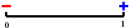
|
|
f(.5)=–.3775..., so we now know there is a
root in the interval [.5,1].
|
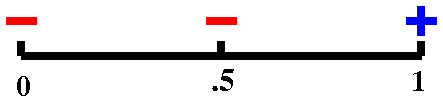
|
|
f(.75)=+.0183..., so we now know there is a root in the
interval [.5,.75].
|
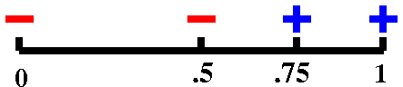
|
|
f(.625)=–.1859..., so we now know there is a root in the
interval [.625,.75}
|
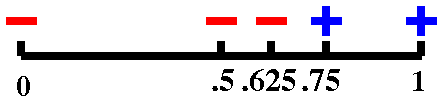
|
| Etc. By this
I mean we can continue chopping the interval, looking for the sign of
f's value at the center, making the length of the interval where a
root is located as small as we like. This is the key idea
of the Bisection Algorithm. The weird entry condition below,
f(a)·f(b)<0, means that f has different signs at the two
ends of the interval.
|
The Bisection Algorithm
Entry conditions
A continuous function f(x) defined on an interval [a,b], with
f(a)·f(b)<0;
a positive tolerance E for the error.
Output
An interval [c,d] so that d–c<E and f(c)·f(d)<0.
This identifies an interval of length less than E
which must contain a root of f(x)=0.
"Loop" structure
Given [p,q] with f(p)·f(q)<0: let m=(p+q)/2. Compute f(m).
If f(m)·f(p)<=0, then replace q by m else
replace p by m.
Exit check If q–p<E then return p and q as c
and d in the output else go to loop.
A simple program implementing the bisection method
Here's a bisection program program written in the Maple programming language. I wouldn't
use this for serious, real applications. Such numerical programs must
have much more careful analysis of the kinds of errors which can
occur and should be carefully tested. I hope the logic is clear.
bisection := proc (f, a, b, E)
   local p, q, m;
   p := a;
   q := b;
   while E <= q–p do
      print(p, q);
      m := (1/2)*p+(1/2)*q;
      if f(p)*f(m) < 0 then q := m else p := m end if
   end do
end proc;
The function f has been defined by the formula f(x)=x–cos(x) in
another statement: f:=x->x–cos(x);. This bisection program
prints out the intermediate stages, so you can see the program
focusing on the interval in which the root sits.
> bisection(f, 0., 1., 0.001);
                                   0., 1.
                              0.5000000000, 1.
                         0.5000000000, 0.7500000000
                         0.6250000000, 0.7500000000
                         0.6875000000, 0.7500000000
                         0.7187500000, 0.7500000000
                         0.7343750000, 0.7500000000
                         0.7343750000, 0.7421875000
                         0.7382812500, 0.7421875000
                         0.7382812500, 0.7402343750
                                0.7392578125
When the program ends, it reports the last variable's value, the
middle of the subinterval.
We will get more sophisticated root-finding methods, but this one is
simple to understand and to use.

Algorithm?
I mentioned the word "algorithm". Let
me give some further information about this word in the form of quotes
from
The Art of Computer Programming by D. E. Knuth:
The modern meaning for algorithm is quite similar to that
of recipe, process, method, technique, procedure, routine,
except that the word "algorithm" connotes something just a little
different. Besides merely being a finite set of rules which gives a
sequence of operations for solving a specific type of problem, an
algorithm has five important features:
- Finiteness An algorithm must always terminate
after a finite number of steps.
- Definiteness Each step of an algorithm must be
precisely defined; the actions to be carried out must be rigorously
and unambiguously specified for each case.
- Input An algorithm has zero or more inputs, i.e.,
quantities which are given to it initially before the algorithm
begins. These inputs are taken from specified sets of objects.
- Output An algorithm has one or more outputs, i.e.,
quantities which have a specified relation to the inputs.
- Effectiveness An algorithm is also generally
expected to be effective. This means that all of the operations
to be performed in the algorithm must be sufficiently basic that they
can in principle be done exactly and in a finite length of time.
Knuth continues on the same page to contrast his definition of
algorithm with what could be found in a cookbook:
Let us try to compare the concept of an algorithm with that of a
cookbook recipe: A recipe presumably has the qualities of
finiteness (although it is said that a watched pot never boils), input
(eggs, flour, etc.) and output (TV dinner, etc.) but notoriously lacks
definiteness. There are frequently cases in which the definiteness is
missing, e.g., "Add a dash of salt." A "dash" is defined as "less
than 1/8 teaspoon"; salt is perhaps well enough defined; but
where should the salt be added (on top, side, etc.)?
... a computer
programmer can learn much by studying a good recipe book
|
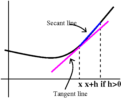
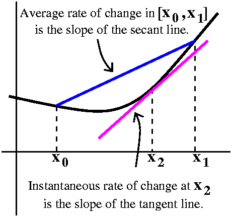 Average and Instantaneous Rates of Change
A few lectures ago I tried to analyze a number of real phenomena. I
hope that background should help you accept the following definitions:
The average rate of change of f in the interval
[x0,x1] is
(f(x1)–f(x0)/(x1–x0).
Geometrically, this is the slope of a secant line connecting the two
points (x0,f(x0)) and
(x1,f(x1)) on the graph of y=f(x). The
instantaneous rate of change of f at x2 is a
stranger thing, that probably can't be physically measured in most
cases. It is the slope of the tangent line at
(x2,f(x2)). The instantaneous rate of change of
f at x2 is better and better approximated by the average
rate of change if the numbers x0 and x1 are
close to f.
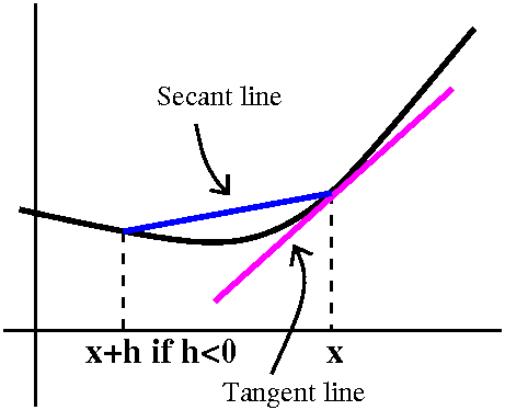
If (x,f(x)) is a point on the curve, then people usually
rewrite the average rate of change using with the secant line joining
the point (x,f(x)) and (x+h,f(x+h)). Below are two views of the
resulting picture, one with h<0 and one with h>0. The official
definition uses this idea of approximating the slope of the tangent
line with the slope of the resulting secant line. In the right-hand
picture, the secant line nearly "overlays" the curve since the curve I
drew is fairly flat there.
The definition
Consider limh→0(f(x+h)–f(x))/h. If this limit exists,
then the value of the limit is f´(x), the derivative of f at
x, and we say that f is differentiable at x.
Most of this course will be devoted to studying the derivative of a
function and its uses. Actually, the next few lectures will show that,
for familiar functions defined by formulas, the derivative can be
computed fairly easily. So computation of derivatives, while both
necessary and useful, is not the ultimate aim of the course (hey, such
computation can be described carefully enough so that [capable]
programmers can create differentiation programs!). We will spend most
of the time investigating how to use derivatives.
Example
A traditional first example is f(x)=x2. Then we need to
consider (f(x+h)–f(x))/h. Let's look at the top of the fraction.
f(x+h)–f(x)=(x+h)2–x2=x2+2xh+h2–x2=2xh+h2=h(2x+h).
In the last step, I factored out an h because I was thinking ahead:
(f(x+h)–f(x))/h=(h(2x+h))/h=2x+h.
Now
limh→02x+h=2x. We're done.
Conclusion The function f(x)=x2 is differentiable at
all x's, and its derivative is given by f´(x)=2x.
A tangent line
What is an equation of a line tangent to y=x2 at x=3? Here
we need a POINT and a SLOPE.
(3,9). If x=3, y=33=9.
f´(3)=2·3=6. The
derivative's value at x=3 is the slope of the tangent line at x=3.
An equation for the tangent line at x=3 is therefore y–9=6(x–3). I'd
probably leave the equation this way unless there was a reason to
change it (if I were requested to provide the answer in a different
form, or if I needed to compute with it more).
 Is it correct?
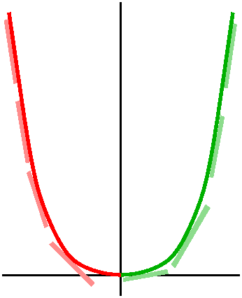
Here I wanted to consider the formula for the derivative,
f´(x)=2x and consider if the answer were reasonable. The
graph of y=x2 to the left of the y-axis is decreasing, and
the tangent lines should be tilted "down". Their slopes should be
negative. And the algebraic candidate we have for the slopes of
tangent lines, 2x, is negative when x<0. On the other side of the
y-axis, the tangent lines tilt "up", and their slopes seem to be
positive. Of course, for x>0, 2x>0.
In this case, considering the answer and seeing that it is reasonable
and consistent with other information is easy. Certainly in more
complicated situations, such checks are more difficult. But if at all
possible, within the limits of time and effort, please try to make
such a check. Everyone makes mistakes: humans, computers, humans using
computers, etc. A few seconds "thought" can catch errors that can be
very irritating later.
And now for xn
Everyone knows the answer. O.k., but why? (Why is "the answer"
actually the answer, not why does everyone know it.) If
f(x)=xn where n is a positive integer, then:
f(x+h)–f(x)=(x+h)n–xn.
We need to consider (x+h)n. It is possible, using the Binomial
Theorem, to write an explicit exact expanded form of this
object. I don't need that. I need much less information. So:
(x+h)n=(x+h)(x+h)···(n times)···(x+h).
There are lots of ways to multiply things out here: you need to choose
in each factor either the left (x) term or the right (h) term. But how
may ways are there which would get only x's? For this, we would need
to make only the x choice each time. There is exactly one way to get
all x's, so xn would only come out one time. How many ways
would result in one h and all the rest (n–1 of them) x's? Well, we
could choose the h from the first term and choose all x's from the
other terms. Or we could choose an h from the second term and all the
others (the first term and the terms after the second term)
x's. Etc. Here by "Etc." I mean that we could take an h from exactly
one of n factors, with all the other choices being x's. So since there
are n factors, there are n ways to get a product with one h and all
the rest x's. So in the result, there's nhxn–1. What about
the rest? We took care of the "no h" term and the "one h" terms. So
all the rest has at least two factors of h. So, actually, we now know:
(x+h)n=xn+nhxn–1+h2JUNK.
In this expression "JUNK" is not something bad. It represents terms I
don't need to care about at this time. In fact, later in the course,
we will try to understand some aspects of JUNK and how they can be
useful. Anyway, let's continue:
(x+h)n–xn=xn+nhxn–1+h2JUNK–xn=nhxn–1+h2JUNK=h(nxn–1+h(JUNK))
where again I factored the h out because I was thinking ahead. Now the limit:
limh→0(f(x+h)–f(x))/h=limh→(h(nxn–1+h(JUNK)))/h=limh→0nxn–1+h(JUNK)=nxn–1.
Therefore, f(x)=xn is differentiable, and its derivative,
f´(x), is nxn–1.
QotD
If f(x)=1/x, use the definition of derivative to find f´(x).
So f(x+h)–f(x)=1/(x+h)–1/x=(x–(x+h))/((x+h)x)=–h/((x+h)x) and
limh→0(f(x+h)–f(x))/h=limh→0[–h/((x+h)x)]/h=limh→0–1/((x+h)x)=–1/(x·x)=–1/x2.
Interesting aspects of this computation: if f(x)=1/x, then
f(x+h)=1/(x+h). You must understand the grammar (?) of functions to do
this. And combining the fractions and converting to a simple fraction:
you must know how to do this sort of algebra.
| Thursday,
September 17 | (Lecture #5) |
|---|
A function f is continuous at x=a if
the domain of f includes an interval surrounding a, and if
limx→af(x) exists, and if the value of that limit is
f(a). In other words, the function is continuous at x=a if the limit
of the function as x "approaches" a is gotten just by plugging in a to
f: computing f(a). Due to many facts about limits (I will mention only
a few here, so please look in the book), most familiar functions are
continuous in their domains.
An absurd example
What is
          1        1
        ----  –  ------
        3x+4      x2+6
 lim  -------------------
x→2          x–2
As I remarked in class, I can't imagine a situation where this
specific limit would occur. But let me try to evaluate it anyway.
"Plugging in" x=2 gets 0 on the bottom, and on top, if we substitute
correctly, 1/(3x+4) becomes 1/10 and 1/(x2+6) becomes
1/10. So the top is (1/10)–(1/10) which is 0. Surprise (not!): this is
a 0/0 situation. We use some algebra. My feeling is great dislike for
compound fractions, that is, fractions within fractions. I find them
difficult to understand and difficult to manipulate. My advice is to
change them into "simple" fractions, where only one division sign will
appear. But we need to do this carefully.
The top is 1/(3x+4)– 1/(x2+6) which is
(x2+6)–(3x+4)
-------------------
(x2+6)(3x+4)
Notice that this fraction is sitting "on top" of (x–2). We have
something like this:
   A         A      1            A
 -----     ----- · ---        -------
   B         B      C           B·C          A
------- = --------------  =  ---------- =  -----
   C              1                           B·C
             C · ---             1
                  C
So the result in our case is that the compound fraction
becomes the following simple fraction:
(x2+6)–(3x+4)
------------------------
(x2+6)(3x+4)(x–2)
We can look more closely at the top:
(x2+6)–(3x+4)=x2–3x+2=(x–1)(x–2).
There is no accident: the x–2 drops out of the top and the bottom, and
now the resulting fraction is
(x–1)/[(x2+6)(3x+4)]. Take the limit as x→2. The result
("plugging in", using continuity) is
(2–1)/[(22+6)(3·2+4)]. I would leave this answer as
is, but if you need to compute, it would become 1/100.
Limits and algebra
If limx→af(x)=L1 and
If limx→ag(x)=L2 then
•
limx→af(x)+g(x) exists and equals
L1+L2;
• limx→af(x)·g(x) exists and equals
L1·L2;
• (when L2 is not 0)
limx→af(x)/g(x) exists and equals
L1/L2.
QotD (definitely less absurd)
(Please accept my guarantee that this is not absurb, at least
for a little while [2 lectures].)What is
       1     1
      --- – ---
       x2    w2
 lim  --------- ?
x→w    x–w
This is a compound fraction. I will try to convert it to a simple
fraction. Let's look at the top:
(1/x2)–(1/w2)=[w2–x2]/[x2w2]
Just as before, the compound fraction in the original limit becomes
(use the A/B/C stuff):
   w2–x2    (w–x)(w+x)       w+x
--------- = ---------- = - ------
x2w2(x–w)    x2w2(x–w)       x2w2
An easy mistake to make here is somehow losing (?) the minus
sign. Please don't. Then:
limx→w–[w+x]/[x2w2]=–2w/w4.
A weird but not absurd limit
f(x)=|x+5|/(2x+10). So what happens as x→7, for example? The
x+5→7+5=12. The absolute value for x's near 7 give x+5 near 12. The
results are all positive, so |x+5|→12. The bottom, 2x+10, approaches
2·7+10, which is 24. The resulting limit value is 12/24.
There's trouble near –5, though. So what about
limx→–5|x+5|/(2x+10)?
Here there's a real difficulty with absolute value. Recall that |w| is
w if w>0 and |w| is –w if w<0. So |x+5| is x+5 if x+5>0. and
|x+5| is –(x+5) if x+5<0. But x+5>0 is the same as x>–5, and
x+5<0 is the same as x<–5. So put all this together:
 suppose f(x)=|x+5|/(2x+10).
If x>–5, f(x)=(x+5)/(2x+10)=1/2;
if x<–5, f(x)=–(x+5)/(2x+10)=–1/2.
To the right is a graph of f. I don't "know" what the value of f(–5)
should be (computer programs handle this differently, but many report
that trying to evaluate the function at –5 is an error).
Such functions occur when trying to model real situations (hey:
"hit" a plate -- that will be a shock! Or drop a chunk of salt into a
container of water -- that's a shock to the salt concentration!). So
getting some language to describe the behavior is useful.
As x gets close to –5 from the left, the values of f(x) are all
–1/2. So people say that
limx→–5–f(x), the
left-hand limit of f at –5, exists, and they say that the value
of this limit is –1/2.
As x gets close to –5 from the left, the values of f(x) are all
1/2. So people say that
limx→–5+f(x), the
right-hand limit of f at –5, exists, and they say that the value
of this limit is 1/2.
You may be confused at first with the superscript/exponent + and
–. The "+" up there always means "from the right" and the "–" up there
will always mean from the left. In the expression x→–5+ the minus before the 5 means look 5 units to
the left of 0. The plus sign in the exponent means see what happens to
the right of that number (that is, –5), but look close to it.
A piecewise linear graph and some limits
|
I drew a graph similar to what's shown to the right. The idea was to
use the geometric information on the graph to find out what we know
about function values and limits. I also wanted to urge students to
understnad the possibilities of our algebraic "language". So to the
right is a graph of y=f(x). Some questions:
|
 |
- What is f(1)? What is limx→1f(x)? (This is the easy
one!)
I see that the point (1,3) is on the graph of y=f(x). A point is on
the graph if it has the form (x,f(x)), so f(1)=3. Also, as x gets
close to 1, the heights on the graph, the f(x)'s, get close to 3. So
limx→1f(x)=3.
The function y=f(x) is continuous at 1. This is because the
limit as x approaches 1 of f(x) exists, and 1 is in the domain of f,
and the value of f at 1 is equal to the limiting value of f.
- What is f(4)? What is limx→4f(x)? (This is not so
easy.)
Well, f(4)=1 since there a big dot at (4,1). What about the limiting
behavior as x→4? A key part of the idea of limit is that what
matters is behavior near the point but not the behavior at the
point. Now as x→4 from either the right or the left, the height,
f(x), gets close to 2. I think that limx→3f(x) exists,
and that the limit is 2.
Since the limiting value is not equal to f's value at 4, f is
not continuous at 1.
- What is f(2)? What is limx→2f(x)? (A bit stranger.)
If I consider points whose first coordinate is 2, points with
coordinates (2,?), there are no such points on the graph of
y=f(x). So 2 is not in the domain of f. What about
limx→2f(x)? Here the heights of the function depend on
which side x gets close to 2. If x gets close from the left, then
the f(x) values are close to 1. So I know
limx→2–f(x) exists, and its value is 1. But
if x gets close to 1 from the right, the heights, the f(x) values,
seem to get close to 0. So now
limx→2+f(x) exists, and its value is 0. Since
the left and right handed limits do not agree, the (two-sided) limit,
limx→2f(x) does not exist.
Since the limit does not exist, the function can't be continuous
at 2.
- What is f(–1)? What is limx→–1f(x)?
Look at the graph. There's a nice thick dot at (–1,2). Therefore I
conclude that f(–1)=2. The two-sided limit at –1 of f does not
exist. As x gets close to –1 from the left, the f values (f(x) is the
height of the curve) get close to 1. So limx→–1–f(x)=1. Look now at the right side of
x=1. The f(x) values drop go to 2, so I conclude that
limx→–1–f(x)=2.
f is not continuous at –1. To be continuous at –1, all these must
exist and be the same number: f(–1) and the left-hand limit at –1 and
the right-hand limit at –1.
My friend Francine...
 The
Garden State Parkway runs most of the length of New Jersey. Mile
0 is at Cape May, while the other end, mile 172, seems to be close to
Montvale. Suppose that my friend Francine leaves Cape May at 7 AM one
morning, and drives north on the Garden State Parkway. Further,
suppose she arrives at mile 172, the northern end, at, say, 10
AM. Must Francine at some time be at mile 135 (fairly near Busch
campus)? The parkway seal here was "borrowed" from a State of New
Jersey webpage.
The
Garden State Parkway runs most of the length of New Jersey. Mile
0 is at Cape May, while the other end, mile 172, seems to be close to
Montvale. Suppose that my friend Francine leaves Cape May at 7 AM one
morning, and drives north on the Garden State Parkway. Further,
suppose she arrives at mile 172, the northern end, at, say, 10
AM. Must Francine at some time be at mile 135 (fairly near Busch
campus)? The parkway seal here was "borrowed" from a State of New
Jersey webpage.
 We discussed various curves which could represent the position of
Francine on the parkway in terms of miles from the start of the
parkway at time t, in terms of hours elapsed from 7 AM. I tried to
show that our everyday intuition lead to the graph being
increasing (as you travel from left to right, the points on
the graph go up). The graph can have level spots, where Francine pulls
over for a rest stop. Legally Francine isn't supposed to drive
backwards, though.
We discussed various curves which could represent the position of
Francine on the parkway in terms of miles from the start of the
parkway at time t, in terms of hours elapsed from 7 AM. I tried to
show that our everyday intuition lead to the graph being
increasing (as you travel from left to right, the points on
the graph go up). The graph can have level spots, where Francine pulls
over for a rest stop. Legally Francine isn't supposed to drive
backwards, though.
If we believe that motion is continuous (so Francine does not
have a Star Trek transporter or other device) then the graph of
Francine's position goes from (7 AM, 0 miles) to (10 AM, 172 miles)
and therefore the graph must have on it at least one point with
coordinate description (*,135). All of this, by the way, rests on some
complicated assumptions, some of them philosophical (why should
motion be continuous?). Today, though, I believe that motion
is continuous, and therefore at sometime Francine must be at Mile
135. This is all the idea behind the following important result.
Intermediate Value Theorem
Suppose that the function f is
defined and continuous on the interval [a,b]. Then the equation f(x)=y
has at least one solution for every y which is between f(a) and f(b).
Problem #5 in section 2.7
Here's the problem:
Show that cos(x)=x has a solution in the
interval [0,1].
Since I am a picture person, I frequently try to draw a graph or two
to understand what the problem is about. In this case, certainly the graph of y=x is easy to imagine on [0,1]. What
about y=cos(x)? Well, it does help, if you don't have access to a
graphing device, to know that cos(0)=1. I know that cosine drops down
as x increases from 0. What do we know about cos(1)? As one student
declared, cos(1) is both less than 1 and greater than 0. That's
because Pi/2 is about 1.57 and cosine decreases between 0 and Pi/2,
and does not reach 0 until Pi/2. So the graph of
y=cos(x) decreases from (0,1) to (1,cos(1)), and the end point
is somewhere above the x-axis. The mental picture I have built is
shown to the right. I deliberately did not have a graphing
device create an "accurate" display of the situation -- I wanted to
show what we should be able to do inside our own heads.
The picture now encourages me to believe the assertion of the
problem. The text supplies this hint:
Show that f(x)=x–cos(x) has a zero in
[0,1].
The phrase "has a zero in [0,1]" means that there is some root of
f(x)=0 in the interval [0,1]. Well, f(0)=0–cos(0)=–1<0 and
f(1)=1–cos(1). Since cos(1) is between 0 and 1, 1–cos(1) will be
between 1 and 0. So we know that f(1)>0. Since the values at the
endpoints are both positive and negative, I know that 0 is between the
endpoint values. The Intermediate Value Theorem then applies to show
that f(x)=0 has a solution between the endpoints, which are 0 and 1.
Can we locate this root more precisely?
I will show you how to do this next time.
| Tuesday,
September 15 | (Lecture #4) |
|---|
Writeups back to you
Mr. Nakamura and I read the writeups. I was impressed by the clear
investment of time and effort which went into many of them. We would
like you to use your time and effort as well as possible. So
here is one possible solution to the
first question, and some further comments on the solution. Please look
at this.
The idea of limit
Today we begin an official discussion of limit. This is a very useful
idea. There are lots of computations and manipulations which are
related to limits in this course and in many other situations. But I
must be very careful about how class time is used, and I must rely on
you to read the textbook and do homework problems. I will
choose to emphasize ideas in the lectures. I will try to do a
sufficient number of examples to illustrate these ideas, but your own
efforts will be key to getting enough experience and sufficient
familiarity.
Tree growth
Catalogs sell trees with short descriptions which frequently include
such information as "The eventual height of this tree is 40 ft and its
growth rate is 2 ft/yr." What do these numbers mean? We discussed this
for a while.
First approach
If one took the 2 ft/yr literally, then in a century the tree would be
200 ft high, and a bit later (well, quite a bit later!) the tree would
knock down the moon. This is probably not realistic.
Another attempt to understand ...
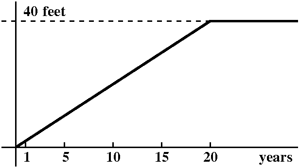 We made a second attempt to understand. The tree would grow at 2
ft/yr, and then, after 20 years (40/2=20) the tree would stop
growing. Well, if we plotted the growth curve, it might look like what
is shown to the right. To me, a simple piecewise linear curve is
really neat and simple. But I don't think this represents behavior of
complex organic objects. For example, I don't think a really tiny tree
would actually grow two feet taller in its first year. I think it
would begin by growing rather slowly. I also don't think that trees
grow at a steady rate, and then tree growth would suddenly and totally
stop at some specific height. That's probably not what happens.
We made a second attempt to understand. The tree would grow at 2
ft/yr, and then, after 20 years (40/2=20) the tree would stop
growing. Well, if we plotted the growth curve, it might look like what
is shown to the right. To me, a simple piecewise linear curve is
really neat and simple. But I don't think this represents behavior of
complex organic objects. For example, I don't think a really tiny tree
would actually grow two feet taller in its first year. I think it
would begin by growing rather slowly. I also don't think that trees
grow at a steady rate, and then tree growth would suddenly and totally
stop at some specific height. That's probably not what happens.
Maybe more real ...
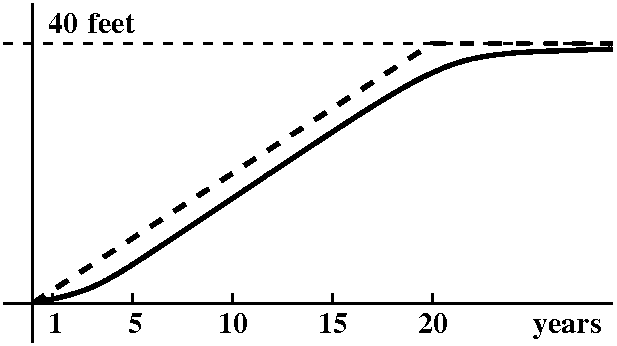 Reality is sloppier. I bet that the tree begins its growth fairly
slowly. Then the growth gets more rapid and steadier, and persists for
quite a while until the tree gets near its "ultimate height". The tree
growth slows then, but I would expect more growth, at a slower rate,
for a while. I think that a more reasonable possibility for a growth
curve is shown to the right.
Reality is sloppier. I bet that the tree begins its growth fairly
slowly. Then the growth gets more rapid and steadier, and persists for
quite a while until the tree gets near its "ultimate height". The tree
growth slows then, but I would expect more growth, at a slower rate,
for a while. I think that a more reasonable possibility for a growth
curve is shown to the right.
In fact, I think what's shown to the right is, itself, only an
imitation of real tree growth. Growth will depend on climate and
weather (moisture, temperature), and nourishment (how much of what
kind of minerals, etc.), and competition (in the shadow of something
else?), and such factors as where is the lumber harvester. Each tree
will likely be somewhat different, and what's presented and described
is an average of many observations.
How could tree growth around, say, year 13, be calculated? Well,
suppose H(t) is the height of the tree in feet, at time t years after
the tree seed germinates. Then we could measure the height of the tree
once a year. So we'd have values for H(12) and H(13) and H(14),
etc. The growth rate in feet per year for the year [13,14] would be
(H(14)–H(13))/(14–13). This number would represent the average
growth rate of the tree during that year. Of course, we could want
more precise information. I could imagine someone measuring the tree
height every 3 months, a quarter of a year. The interval [13,13.25]
would be closer to 13. And I would think that the quantity
(H(13.25)–H(13))/(13.25–13) would be a better idea of what might be
the tree growth rate "at" 13. Of course, this fraction is what's
called the average growth rate in the interval [13,13.25]. We could
imagine an enthusiast desiring better information. This person could want
10,000 measurements of the tree height during the year, etc. This
information could be used to give more precise information about tree
growth rate. Now think about real life. I don't believe that 10,000
tree measurements are likely. I think that approximate
average rates
of growth are all we can expect, and the idea of some totally precise
"growth rate" is fictional. But, even though it is fictional, such an
ideal growth rate may be useful.
 Rock dropping
I used feet and pounds, an antique system of measurements in this
discussion. This may be confusing. I am sorry.
Suppose we drop a rock. Then the rock will fall approximately
s(t)=16t2 ft after t seconds. If we wanted to know the
average velocity that the rock fell in the one second after t=3, we
could compute:
s(4)–s(3)  16(42)–16(32)
-------- = ------------= 16(16–9) = 112
 4–3             1
The units in this answer are ft/sec. I am dividing the distrance
traveled by the time elapsed. So, on average, the rock fell 112 ft/sec
during the time interval [3,4]. Suppose I wanted to get a better
estimate of the average velocity near time 3. I could measure the
distance at, say, t=3.007. Then since (3.007)2=9.042049,
the average velocity of the rock during the time interval [3,3.007]
would be
 s(3.07)–s(3)    16(9.042049)–16(9)      16(.042049)
------------- = --------------------- = ------------- = 96.112
  3.007–3              .007                .007
So
this average velocity, which, with some effort, I could
actually imagine observing and measuring and computing, is 96.112:
that is, on average during the time interval [3,3.007], the rock fell
96.112 ft/sec.
Let's now use algebra. Algebra allows almost everyone to be clever. So
we can ask: what is the average velocity of the rock during the time
interval [3,3+h] if h is a small positive number? The computation
would be something like this:
s(3+h)–s(3)    16(3+h)2–16(32)   16(9+6h+h2)–16·9    16(6h+h2)
------------ = --------------- = ---------------- = ---------- =16(6+h)
    h              h                  h               h
So the average velocity of the rock during the interval
[9,9+h] seconds is 16(6+h) ft/sec.
This is actually a rather remarkable computation, and just because you
may have seen such things before is no reason to ignore the wonder:
you must be like a child .... Let's check the formula. If
h=.007, then 16(6+h) is 16(6.007)=96.112 (that's what we got
before). To me, the most remarkable part of the computation is that we
have a quotient, a tiny distance change on top, and a tiny time change
on the bottom. Amazing, somehow the "tiny"'s sort of cancel, and we
are left with an average velocity, 16(6+h), which has a sort of
stability property as h gets smaller. In fact, if you don't think too
hard, as h gets smaller ("h→0") then 16(6+h) gets close to 16(6)=96
("16(6+h)→96").
So the average velocity over the interval [3,3+h] approaches 96 as the
length of the time interval goes to 0. People abbreviate this by
declaring that 96 is the instantaneous velocity of the rock at time
3. As far as I know, human beings don't actually measure or observe
instantaneous velocities. These instantaneous things are lies, o.k.,
we shouldn't call them lies, they are useful fictions or mental
constructions. Most of this course will be about such useful fictions.
Local linearity
Last time we considered the curve y=3x
and zoomed in on it around the point (0,1). We observed that the curve
seemed more and more to appear like a straight line. Hey: I even gave
this phenomenon a name: local linearity. The line goes through the
point (0,1), and therefore complete information about it only depends
on knowing its slope. Well, if we think that the line is about the
same as the curve, on a very very small scale, then maybe another
point on the line would approximately be (h,3h) if h is a
small positive number. The slope is then the difference in the second
coordinates divided by the difference in the first coordinates:
(3h–1)/h (on the bottom, h–0 is just h). In this case,
unlike the low-degree polynomial investigated with the rock, the h's
don't obviously somehow fade away. We guessed using numerical evidence
that as h→0, this quotient also "stabilizes" near the value
1.1. This behavior is not obvious to me algebraically, and, indeed, if
I wanted to verify it for you right now, showing the limiting behavior
would take a great deal of effort.
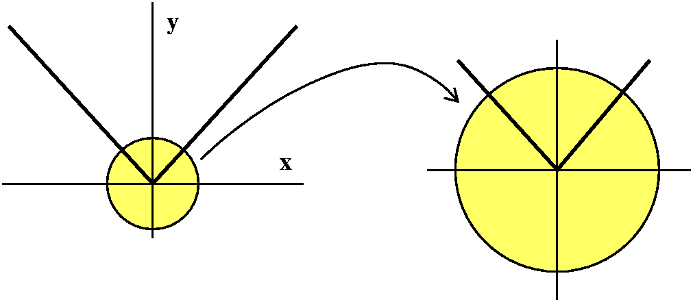 A function which isn't locally linear
Look at the graph to the right, and specifically look "near"
(0,0). Here I am deliberately omitting the scale marks on the axes,
because they don't matter for the purposes of this discussion. If we
zoom in around (0,0), we get something which looks much the same. This
is a self-similar object and scale doesn't matter. (Self-simlarity
is a key part of what are called fractals, one natural
(?) appearance of which is here).
There's no magnification which will make the graph to the right look
like a straight line through the point (0,0). So this is a graph of a
function which is not locally linear. In this course, most of
the functions we will consider will be locally linear, so you should
see that some rather simple graphs will just be thrown out of
consideration.
Please realize that the graph to the right is associated with |x|, and
is not an abstract, weird invention.
Observations and ideals
We, humans, can observe average rates of change. We can measure how
balls roll down inclined planes. We can, with considerable more
ingenuity and equipment (go over to the Chem Department!) make
observations of chemical reactions on a near-nanosecond scale. As far
as I know, we look at average rates of change. A nice invention
is the instantaneous rate of change, which will be a principal
object of study in this course. As far as I know, we do not observe
instantaneous rates of change. We can only approximate them by real
measurements. This course studies the useful fictions related to
instantaneous rates of change.
Notation
I introduced some notation to help us talk about average and
instantaneous rates of change. We will want to study the behavior of
some function f(x) when x gets close to a, and, in particular, we will
want to tell people that (in "good" cases) f(x) gets close to b when x
gets close to a. Well, arrows are usually used to abbreviate "gets
close to". So we want to declare that as x gets close to a, f(x) gets
close to b, and we will write for this "As x→a, then f(x)→b."
An even more compact (lazier!) way of stating this is to write
limx→af(x)=b and this is how I'll communicate this
complicated "gets close to" idea.
Basic method: plug in
Suppose you want to understand limx→af(x). If the
function is defined by some formula you understand and believe is
well-behaved, plug in. That is, evaluate f(a).
Example What's limx→3x2? I think it is
32.
This "trick" is important enough so that there is a label which goes
with it. A function f is continuous at x=a if the domain of f
includes an interval surrounding a, and if limx→af(x)
exists, and if the value of that limit is f(a).
In other words, the function is continuous at x=a if the limit of the
function as x "approaches" a is gotten just by plugging in a to f:
computing f(a). Due to many facts about limits that we will mention
next time, most familiar functions are continuous in their domains.
Many of the most interesting limits we need to deal with (those
involving rates of change, for example) can't be evaluated by
just plugging in. Here are two examples:
limx→0(3x–1)/x and
limx→0(sin(x))/x. In both cases, plugging in gives
0/0. In fact, both limits do exist. The value of the first one is
ln(3) and the value of the second one is 1. Neither fact is obvious,
and some effort is needed. But sometimes limits can be seen by
(relatively!) simple algebraic manipulation. We will try to change
them into forms which can be evaluated by "plugging in".
Next method: algebraic transformation, with the goal being ...
Sometimes (fairly frequently in this course) we will need to find some
limit but the "plugging in" gives us 0/0, and I don't know how to make
sense of this quotient. So one thing we can try is to change the given
expression algebraically and maybe get something which is equal but
which does permit plugging in.
Example I think we looked at the more complicated example:
limx→4(x–4)/(sqrt(x)–2).
Here plugging x=4 in just gets you 0/0, which I don't understand. I
can see two ways of analyzing the fraction inside the limit.
Method 1 Multiply by the conjugate.
Be sure to multiply by the same thing on the top and bottom, or else
the result might not be equal! Here this means:
     (x–4)               (x–4)(sqrt(x)+2)            (x–4)(sqrt(x)+2)
----------------- = ----------------------------- = ------------------- = sqrt(x)+2
  (sqrt(x)–2)          (sqrt(x)–2)((sqrt(x)+2)           x–4
Therefore
limx→4(x–4)/(sqrt(x)–2)=limx→4sqrt(x)+2
which we can handle by plugging in x=4, so the answer is
2+2=4.
Method 2 Another way of handle the quotient which some people
prefer is this:
    (x–4)         (sqrt(x)–2)(sqrt(x)+2)
-------------- = ------------------------- =sqrt(x)+2
  (sqrt(x)–2)        (sqrt(x)–2)
Then again
limx→4(x–4)/(sqrt(x)–2)=limx→4sqrt(x)+2=2+2=4.
To me the second method has always seemed more difficult and I can't
tell you why. Maybe this is because the top has to be "recognized" as
a product and this may not be easy.
Use any valid method that works for you, please. Here's another
view of conjugation
QotD
What is
limx→1(x2–5x+4)(x2–3x+2)?
Plugging in gets
(12–5+4)(12–3+2) which is a 0/0 form and doesn't
tell us anything. But a number of people called out, "Factor" as a
hint.
(x2–5x+4)(x2–3x+2)=[(x–4)(x–1)]/[(x–2)(x–1)]=(x–4)/(x–2)
when x≠1.
Therefore
limx→1(x2–5x+4)(x2–3x+2)=limx→1(x–4)/(x–2)=(1–4)/(1–2)=3.
| Thursday,
September 10 | (Lecture #3) |
|---|
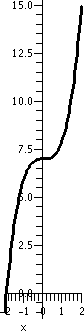 Functions and their inverses
Consider the function f(x)=x3+7. A graph of this function
is shown to the right. I hope you recognize this as x3
moved up 7 units. Certainly f(2)=23+7=15: the output
corresponding to the input 2 is 15. Since f is a function, 15 is the
unique, the only output corresponding to the input 2. But the function
f has an interestping property. Suppose f(x)=15. This means
x3=7=15 so x3=15-7=8. And x=81/3=2. The
only input corresponding to the output 15 is the input 2. The
geometric interpretation of this is gotten by considering the
horizontal line y=15. This line intersects the curve y=x3+7
at exactly one point, (2,15). In fact something more general is
happening.
The specific function f considered here is one-to-one (1-1). This
means there is exactly one distinct input for each output. How can we
verify this? If you believe the graph, the fact means that any
horizontal line will intersect the curve at most one
time. Algebraically, we can do this: y=x3+7 implies that
x=(y-7)1/3. If y is the output, we have just "constructed"
the input, x, corresponding to the output, y.
One-to-one
If we have a 1-1 function, we can think about reversing the process,
and the reversed process is the inverse function to the
original function. Right now the idea is what I'd like to make sure
of. There are certainly implementational issues to worry about, and
these aren't easy. But I think the idea should precede computations in
this case. The ludicrous diagram to the right is supposed to make
clear (?) what's going on. If there is exactly one output value
corresponding to each input value, then we could think about reversing
this association, and creating an inverse function.
In the case of f(x)=x3+7 I know that f is 1-1 because I can
solve f(x)=y and get exactly one value of x for each y. The function
g(y)=(y-7)1/3 is a function defined by the algebraic
formula I got while solving. It is a formula for the function inverse
to f.
If the point (x,y) which is (f's input, f's output) is on the graph of
f, then (y,x) will be on the graph of the inverse to f. The switch
(x,y) to (y,x) is geometrically done with a flip across the "main
diagonal", y=x.
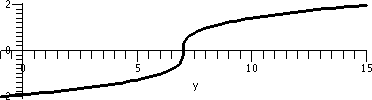
Part of the graph of the function inverse to this f(x)=x3+7
is shown to the right. It is the cubic curve flipped over the main diagonal.
Squaring
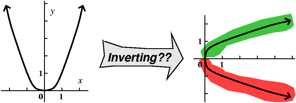 Consider squaring: f(x)=x2. We know about this function. It
is perhaps the most obvious (once the negative numbers are learned)
example of a function which is generally (except for 0) not
1-1. Look: f(2)=22=4 and f(-2)=(-2)2=4
also. Take the graph, a parabola whose vertex is at (0,0), and flip it
over the main diagonal. The result is a curve which is not the graph
of a function. "Everyone" knows this. Yet at the same time everyone
would like to indicate square roots, and would like to tell that the
square root of 4 is ... well, it could be -2 or +2. If a unique output
is desired, the unique output which people have chosen is the
non-negative answer (a classical word for this was "branch", really,
apparantly because the flipped over curve might look like it has
several slanting tree things). So sqrt(x) (really, better written with
that strange almost-division sign) means the non-negative number whose
square is x. So there has been a choice, in terms of the graph shown
to the right. "Everyone" has decided to take the top, green, piece of
the graph, and if ever the bottom part has to be used, it will be
designated -sqrt(x).
Consider squaring: f(x)=x2. We know about this function. It
is perhaps the most obvious (once the negative numbers are learned)
example of a function which is generally (except for 0) not
1-1. Look: f(2)=22=4 and f(-2)=(-2)2=4
also. Take the graph, a parabola whose vertex is at (0,0), and flip it
over the main diagonal. The result is a curve which is not the graph
of a function. "Everyone" knows this. Yet at the same time everyone
would like to indicate square roots, and would like to tell that the
square root of 4 is ... well, it could be -2 or +2. If a unique output
is desired, the unique output which people have chosen is the
non-negative answer (a classical word for this was "branch", really,
apparantly because the flipped over curve might look like it has
several slanting tree things). So sqrt(x) (really, better written with
that strange almost-division sign) means the non-negative number whose
square is x. So there has been a choice, in terms of the graph shown
to the right. "Everyone" has decided to take the top, green, piece of
the graph, and if ever the bottom part has to be used, it will be
designated -sqrt(x).
Choosing an inverse
In this case the choice of a part of the function's domain and the
inverse has been done in our culture years and years ago, and I think
it is likely we have all grown up with it so nicely that we haven't
thought about it!
The trig functions and their inverses
The six trig functions are all periodic. Therefore the difficulties of
squaring actually become much more obvious. If sin(θ)=1/2, well, then, actually, θ could be Π/6 or 5Π/6 or Π/6-2pi
or 5Π/6-2Π or Π/6+2Π or 5Π/6+2Π or ... actually infinitely many
other possibilities. Yet if you are interested in numbers,
solving equations like sin(θ) =some number for θ
might be important (hey, I mentioned in class and meant the following:
construct a robot arm, and "watch" its motion -- you'd better be able
to understand how the values of the input and output of sine and
cosine work!).
arcsine
People have agreed to "restrict" the domain of sine to
[-Π/2,Π/2]. Then the function is 1-1, changing the inputs
[-Π/2,Π/2} to putputs [-1,1} (sine is increasing in that domain, and
we will develop techniques to verifty such claims easily). So there is
an inverse function. The text calls it sin-1 and I will try
not to use that notation since a -1 in the exponent makes me think of
reciprocal. The notation I will use is arcsin. Also I should
mention that most of the computer languages I know use the designation
arcsin to mean what I am describing here
(since superscripts are difficult to type!). The graph to the right is
arcsin. The endpoints are (-1,-Π/2) and (1,Π/2). Everyone agrees
that the domain of arcsin is [-1,1] and the range is [-Π/2,Π/2].
| 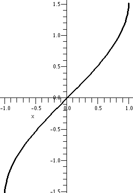
|
arctan
 Tangent, from the inverse function point of view, is in some silly
sense twice as bad as sine. ! This is
because sine is 2Π periodic and tangent is Π periodic. The tangent
domain restriction that people use almost always (99.999% of the
time!) is (-Π/2,Π/2). The open interval results from the fact than
tangent is not defined at odd multiples of Π/2 (hey, cosine is 0
there). So flip the graph of tangent. The result is arctan (or, in the
text, tan-1).
Tangent, from the inverse function point of view, is in some silly
sense twice as bad as sine. ! This is
because sine is 2Π periodic and tangent is Π periodic. The tangent
domain restriction that people use almost always (99.999% of the
time!) is (-Π/2,Π/2). The open interval results from the fact than
tangent is not defined at odd multiples of Π/2 (hey, cosine is 0
there). So flip the graph of tangent. The result is arctan (or, in the
text, tan-1).
The domain of arctan is all real numbers. The graph is
increasing, and when x gets very large positive, then arctan(x) gets
close to Π/2. On the other side, when x gets very large negative,
then arctan(x) gets close to -Π/2. There are two (horizontal)
asymptotes, y=Π/2 and y=-Π/2. As I mentioned, arctan is used to take
big positive and negative numbers and output numbers which are more
controlled, between -Π/2 and Π/2. arctan has been more used by me
than tan. It is a neat function.
Building powers of 3
I gave an extended discussion of exponents. The aim was to explain my
view of how the "exponent laws" were created (invented?). I do not
know if, in fact, what I discussed is supported by historical data.
36 means
3·3·3·3·3·3. That is, 3's repeated
and multiplied 6 times. Therefore
RULE
3positive integer means 3's multiplied together that
"positive integer" number of times.
Then, surely, people noticed things like 35+2 is
37, seven 3's multiplied, and this is the same
(associativity) as 35·32: just line
things up and multiply them.
RULE If n and m are
positive integers, then
3n+m=3n·3m.
Well, then, this "rule" is neat and easy to remember. But consider the
following "equation" (quotes because until you decide what some of the
symbols mean, the equation is silly):
36=36+0=36·30. If
this equation is valid, then 30 should mean 1. Making this
equation correct would mean that the simple template just above would be
true for n and m non-negative integers, and then I (and other
people) would have less to remember.
RULE 30=1.
If we want to extend the n+m equation more, consider the following
"equation" (quotes again because we are exploring how the symbols
work):
30=37-7=37+(-7)=37·3-7.
Then since we want 30 to be 1,
1=37·3-7 so that
3-7=1/37. Well, then, here's another
definition:
RULE If n is a positive
integer, then 3-n=1/3n.
So, for example, 3-2 must be 1/9. Finally, what happens if
we repeat exponentiation? Let's consider (34)2. What
is this? Well, 34 is 3·3·3·3 (four 3's
multiplied). Then squaring this gets us
(3·3·3·3)·(3·3·3·3). If
you count this is eight 3's multiplied: 38. So therefore
(34)2=38. Therefore we get
another:
RULE If n and m are positive integers, then (3n)m=3n·m.
But what about, say, 37/2? If we believe in the previous
result, or, better, we want to use it as a simple template for
computation, then consider (31/5)5. This "should" be
3(1/5)·5=31=3. So therefore
31/5 should mean the positive number which is the fifth
root of 3, the unique positive number which solves x5=3.
RULE If n is a positive
integer, then 31/n is the nth root of 3, that
is, the positive solution of xn=3.
People have adapted these rules so that exponentiation is easy to handle.
If b is a positive number, then:
- bn=b·b·...·b
n times.
- b0=1.
- bp+q=bp·bq.
- b-p=1/bp.
- (bp)q=bp·q.
Although maybe these rules are all "obvious" to you, in fact I hope
that you see they are designed so people and numbers live together
comfortably. To a certain extent, math is a human
construction. Certainly mathematical notation is human. The
obviousness is partly due to your constant exposure to such equations
(since maybe fifth or sixth grade?). I remarked that the repeated
exponentiation equation, obvious and clear, is an important part of
RSA encryption, a very widely used method for secure electronic
communication (for example, commercial web transactions). Google has two and quarter million links to
the phrase "rsa encryption".
|
The definition (?) of 3sqrt(2)
I mentioned this in class, although I suspect it seemed weird and
totally useless to most students. Very briefly, the problem is how to
define and compute such things as 3sqrt(2). The previous
discussion showed how to compute, say, 377/17 First find
the 17th root of 3 and then take the 77th power
of that root. But sqrt(2) is not rational. It can't be written as a
quotient of two integers. Numbers like 3sqrt(2) will occur
in calculus, and we may want to get some approximation of them. So
what's done? First, get an approximation of sqrt(2): 1.414213562, for
example (!). This is rational (you may not like it, but it is
1414213562/100000000. Then compute 31.414213562 which is
about 4.728804386. And this is what is done.
The curve y=3x investigated
I asked people to graph y=3x on their graphing
calculators. Below are some results.
| To the right is a graph of y=3x in the window
-1<=x<=1, 0<=y<=2. I think the curve looks sort of the way
everyone thinks it should. This window has the point
(0,30), which is (0,1), in the middle of it. |
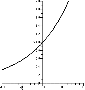
|
| Please keep track of the dimensions of the window. Here I've
"zoomed in". The window is -.25<=x<=.25,
.75<=y<=1.25. This is again a square window. The zoom is a
factor of 4. The bend in the curve is still visible to me, but the
amount of curviness is less.
| 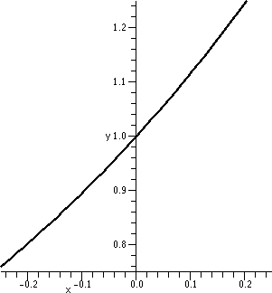
|
|
The zoom is higher. Now the square window has these
dimensions: -.01<=x<=.01, .99<=y<=1.01. The curve is, to
my weak human eyes, just about flat. The phrase "locally linear" is
used for functions like 3x. This phrase means that if the
graph of the function is zoomed at enough, the result looks very much
like a straight line. In fact, the functions of interest in this
course will be exactly the locally linear functions.
The straight line, if you look at it carefully (some students did) has
slope approximately equal to 1.1. (Hey,
(3.05-30)/(.05-0) is about 1.12).
|
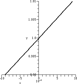
|
|
You can go through the same sequence of graphs for
y=2x. I'll skip to the third graph. So what's shown to the
left is the third result, which is y=2x in the window
-.01<=x<=.01, .99<=y<=1.01. Again, this curve is locally
linear, and the window is sufficiently small so that the piece of
graph visible looks to me like a segment of a straight line. The slope
of this line is about .69. (A computed value of
(2.05-30)/(.05-0) is about .705.)
|
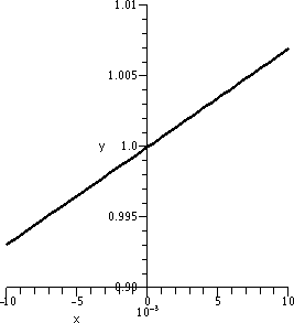
|
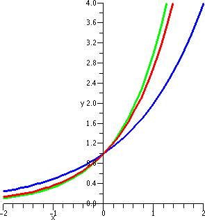 Exponential functions are very commonly used to model such phenomena
as radioactive decay and bacterial growth and lots of other
things. The local linear approximations are things we will work
with. I don't find 1.1 ("slope" of 3x near (0,1)) and .69
("slope" of 2x near (0,1)) particularly nice numbers to
work with. I would rather work with 1. We
can adjust the local slope of bx by varying b. There is a
unique number b (between 2 and 3) so that the local slope of
bx at (0,1) is 1.
Exponential functions are very commonly used to model such phenomena
as radioactive decay and bacterial growth and lots of other
things. The local linear approximations are things we will work
with. I don't find 1.1 ("slope" of 3x near (0,1)) and .69
("slope" of 2x near (0,1)) particularly nice numbers to
work with. I would rather work with 1. We
can adjust the local slope of bx by varying b. There is a
unique number b (between 2 and 3) so that the local slope of
bx at (0,1) is 1.
This number is called e. To the right is a graph of 2x in blue and 3x in green and ex in red. The graph does show
ex "sandwiched" between the other two exponentials. It
doesn't clearly show that ex has the desired local slope of
1, but this is actually true. We will later see how to compute e with
as much accuracy as desired. ex is widely known as
the exponential function, and frequently referred to as exp(x).
e is approximately 2.71828, and I sort of doubt that more digits will
be needed by almost anyone in the class for practical computation. e
is not rational, and its decimal expansion does not repeat. If you
wish, here
are about the first 2 million decimal places of e. People have
computed billions of decimal places of both e and Pi. What else
is there to do?
| Thursday,
September 3 | (Lecture #2) |
|---|
Remember: Tuesday is Monday! I discussed the workload of 153
and how to get through a math lecture. (Stay awake, take notes, and
ask questions!)
Geometry
The real numbers are usually thought of as corresponding to a specific
geometric object, the real line. I think of this line
as horizontal with 0 sitting "in the middle". 1 is to the right of
0. And this geometric picture brings up the idea of order. In addition
to the algebraic structure, there is order: a<b. To me this means
(in my picture of the line) that a is to the left of b. Negative
numbers are to the left of 0 and positive numbers, including all the
positive integers, are to the right of 0. Here are some interesting
aspects to note.
Distance including a discussion of | |
The distance between two points is a non-negative real number whose
size expresses how far apart the numbers are. This will be important
when we study approximation schemes. We'd like to know that the
approximation gets "close" to the correct answer, and the closeness
will be measure by the distance. Algebraically, if the points
correspond to the real numbers a and b, the distance between them is
|a-b| and this is the same as |b-a|, so that distance has some
symmetry. But I just used absolute value, and here is the
piecewise definition of absolute value:
|x|=x if x≥0 and |x|=-x if x<0
Therefore absolute value is always a non-negative number. The absolute
value of a number is 0 only when the number itself is 0. And absolute
value of a product is the product of the absolute values (this
actually is not totally obvious, and needs a bit of thought, I
believe). That is, |ab|=|a|·|b| is always true. But addition doesn't work as well. That is,
|a+b| and |a|+|b| need not be the same. Try a=4 and b=-1, for
example. Then |a+b|=|4-1|=|3|=3 and |a|+|b|=|4|+|-1|=4+1=5. So some
care is needed because such expressions will occur in this course and
we need to know what are and are not legal manipulations.
Intervals
Suppose we want to discover what numbers x are closer to 9 than a
distance of 4. Algebraically this requirement translates to
|x-9|<4. We can sort of "unroll" the inequality. The absolute value
will be less than 4 if the number itself is both less than 4 and
greater than -4. The two inequalities can be compactly written as
follows:
-4<x-9<4 which implies 5<x<13.
This is an interval and an interval which does not contain
either endpoint is called an open interval. The notation for
this interval is (5,13). Intervals which
contain both endpoints are called closed. An examples of such
an interval is [-4,6], which means the numbers x satisfying
-4≤x≤6. There are also
half-open intervals, unbounded intervals (with notation using + or -
∞), etc. Please see the textbook.
Warning!
If you wanted to "solve" (better: understand!) the inequality
|x-9|>4 you can't just "unroll" it to -4>x-9>4. This
inequality has no solutions. There is no number
which is simultaneously less than -4 and greater than 4. You
can't write this so compactly and using such implications represents
an invalid (wrong!) method of solution.
A valid method of solution would involve separately solving
the inequalities:
-4<x-9 or x-9>4 which gives
5<x or x>13. This is actually, therefore, two
intervals:
(-∞,5) and (13,∞). So the inequality
|x-9|>4 has a solution set which is two intervals.
The plane
The conventional way to describe the plane algebraically is to drop
down two lines perpendicular to each other: coordinate axes. A point
in the plane will then be described by an ordered pair of real
numbers. The first coordinate will usually be called the x-coordinate
and the second, the y-coordinate. This pair describes ordered
distances from the horizontal (the x-axis) and vertical (the y-axis)
lines. Please see the text for more about this.
The embarrassment of all this, especially with "new" students, is that
(3,8) could describe both a point in R2, the plane, and
could also describe an open interval (with [missing!] endpoints 3 and
8). The context is supposed to help, but still the notational
confusion is possible, and this is lousy.
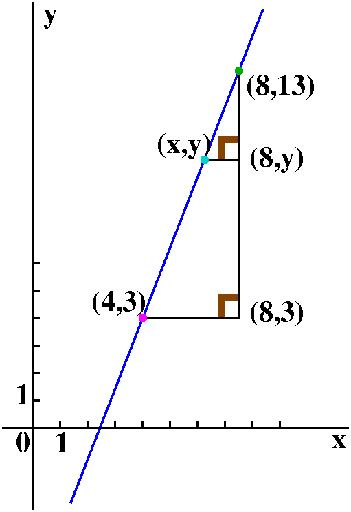
A (non-vertical) line and its algebraic description
Suppose we wanted an algebraic description of points with coordinates
(x,y) which lie on the straight line which goes through (4,3) and
(8,13). If (x,y) is such a point, then look at the picture: two right
triangles indicated are similar, so the corresponding sides have the
same ratios:
13-y   13-3
---- = ----
 8-x    8-4
and the point (x,y) is on the line exactly when
y-13=([13-3]/[8-4])(x-8). The quantity ([13-3]/[8-4]) is called the
slope, and multiplies changes in x to give changes in y. It is
frequently designated with the letter m.
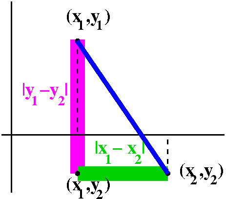 Distance in the plane, R2
Look, please, at
the diagram to the right. In the plane, points correspond to ordered
pairs of numbers. So a point p might correspond to an ordered pair,
(x1,y1), and q might correspond to (x2,y2). Then the point (x1,y2) is
the vertex of a right triangle whose hypotenuse is a line segment
connecting p and q. One leg of the right triangle is on a line where
all the first coordinates are x1, and the length of that leg is given
by the one dimensional formula, |y1-y2|. The other leg is on the line
where all the second coordinates are y2, and the length of that leg is
|x1-x2|. Then by Pythagoras, the hypotenuse has length
sqrt(|x1-x2|2+|y1-y2|2). And usually the
absolute values are discarded since we are squaring the
quantities. Therefore we officially define:
dist(p,q)=sqrt((x1-x2)2+(y1-y2)2) if p
has coordinates (x1,y1) and q has coordinates (x2,y2).
|
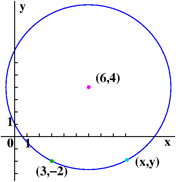
Example
The distance between between (3,-2) and (6,4) is
sqrt([3-6]2+[4-(-2)]2)=sqrt(32+22)=sqrt(13).
A point (x,y) is on a circle of radius sqrt(13) centered at (6,4)
(shown to the right) if sqrt((x-6)2+(y-4)2)=sqrt(13). People usually square this so it looks
nicer, and the result is (x-6)2+(y-4)2=13
Functions
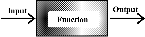 The word function is used in a technical sense in calculus, and
is one of the most important vocabulary words. It is the logical
setting for how things are transformed to other things. In the case of
Math 153, the "things" are numbers. So functions will change numbers
to numbers. A function is a rule changing numbers to numbers, with the
important restriction that each "input" number is assigned a unique
output number. You could think of a function as a machine with an
input and a unique output associated to each input. The collection of
all valid inputs to the machine, those inputs which don't cause the
machine to break, is called the domain. The collection of all
of the outputs for these valid inputs is called the range.
The word function is used in a technical sense in calculus, and
is one of the most important vocabulary words. It is the logical
setting for how things are transformed to other things. In the case of
Math 153, the "things" are numbers. So functions will change numbers
to numbers. A function is a rule changing numbers to numbers, with the
important restriction that each "input" number is assigned a unique
output number. You could think of a function as a machine with an
input and a unique output associated to each input. The collection of
all valid inputs to the machine, those inputs which don't cause the
machine to break, is called the domain. The collection of all
of the outputs for these valid inputs is called the range.
One example, from the toy model, already tricky!
In the toy model of paper folding I mentioned last time, we got the
equation V=x(11-2x)(8-2x). Here x represented the side length of the
"excluded" corner squares, and V was the volume of the resulting
container. Well, the formula on the right side of the equation defines
a function. Usually we write V(x) to show the dependence of V on the
input value, x. So V(x)=x(11-2x)(8-2x). What is the domain of this
function, V? If we just consider the formula, we'll get one answer:
the polynomial has a value for all x's. The "natural domain" of a
function defined by the formula x(11-2x)(8-2x) is all x. But if the
formula is being used to model the physical situation, then there are
definite restrictions on x. Certainly x should not be negative (cut
out a square with
negative sides?). And x can't be bigger than half of the
smaller side length (remember that the paper's original size was 8 by
11 inches). So the domain is (0,4). Some people (many people,
actually) argue that it makes more sense for the domain in this model
to be [0,4]. I won't continue this discussion now, but we will come
back to it. But certainly the physically reasonable domain for V in
this problem is not the same as the "natural domain".
The range of V is interesting. If we allow x=0, the range
"begins" at 0. How big does it get? I don't know now. So the
range of V is [0, I don't know now].
The value of I don't know now is
actually the desired largest volume. We'll be able to find this easily
with calculus. I don't know any other way to find this largest volume
easily.
A more complicated function
 If a function is given by a formula, and there are no other
restrictions involved, we will usually assume that the function has
its natural domain, the largest collection of input numbers for
which the formula makes sense. In this course, the most frequently
encountered simple restrictions will be: don't divide by 0 and don't
take square roots of negative numbers (this is a real calculus
course!).
If a function is given by a formula, and there are no other
restrictions involved, we will usually assume that the function has
its natural domain, the largest collection of input numbers for
which the formula makes sense. In this course, the most frequently
encountered simple restrictions will be: don't divide by 0 and don't
take square roots of negative numbers (this is a real calculus
course!).
For example, suppose that the function f is defined by the formula
f(x)=sqrt(x)+sqrt(3-2x). What is the domain of this function? Since
sqrt(x) occurs, I know that x≥0. But sqrt(3-2x) is also present,
so 3-2x≥=0, which is equivalent to 3≥2x which is equivalent to
3/2≥x. Both of the restrictions must be satisfied, so that the
domain is the closed interval [0,3/2] (both endpoints are included).
The graph of a function
The collection of all points in the plane which correspond to the
ordered pairs (x,f(x)), when x is in the domain of the function, is
called the graph of the function. I like pictures, so I like
graphs. Substantial evidence exists (allocation of neural resources --
brain power!) suggesting that humans can process lots of visual clues
efficiently, much more, say, than many numbers or algebraic
formulas.
I asked for a graph of the function we just discussed, with two square
roots. Here I
expected and wanted people to use a graphing calculator!
A computer-drawn graph is shown to the right. Please bring your
calcululators to class.
I don't know the exact range of this function. We'll come back to this
question later.
Another way to specify functions
Very often in real life functions are not given by formulas.
I gave the information in the table to the right. The
table declares values for certain functions (A, B, and C) at certain
inputs (0, 1, and 2). For example, C(2)=4. We computed the
following:
C(B(1))=C(0)=-2 and
B(C(1))=B(2)=5. These results are not equal.
C(1)B(1)=2·0=0 and
B(1)C(1)=0·2=0. These results are equal.
If f(x)=B(x2+x), then
f(0)=B(02+0)=B(0)=-1 and
f(1)=B(12+1)=B(2)=5.
|
|
Here I wanted to stress that tabular information (the collection of
"data points") was enough information to do these problems. Notice,
please, that while multiplication is commutative, composition of
functions is not. Composition is also written with a little
circle. So B(C(1)) can be written BoC(1).
Please note that many functions arise from data points and not from
formulas. Theory suggests formulas but the data points, measured by
engineers and other experimenters, are reality. So don't disregard
this method of specifying functions.
It is also possible to specify a function with its graph. So
that's what I did.
 An example
I drew a curve much like what is displayed to the right. What was
drawn? It was a nice ("continuous", technical word to be defined
later) curve which "interpolated" (was drawn to connect) the five
"data points" (-2,4), (-1,0), (0,-2), (1,-3), and (2,-1). I told
students that this was a graph of the function A (or A(x) if you want
to give an explicit independent variable).
This is the graph of a function, since it passes the
vertical line test: every vertical line intersects the graph at
most one time. This is logically the same as requiring that every
input yields exactly one output.
What is the domain of this function? That's the set of x's for which
there is a point (x,something) on the graph. Look at the collection of
vertical lines which touch this graph. The x's which touch or cross
this graph are all x's in the closed interval [-2,2].
What is the range of this function? That's the set of y's for
which the point (something,y) is on the graph. You can find these by
considering all of the horizontal lines which touch or cross the
graph. Notice, please, that there are horizontal lines which cross the
graph more than once. This is definitely permitted by the definition
of function. There can be distinct inputs which have the same
outputs. The range is [-3,4].
Creating some new functions
- Define the function B by the equation B(x)=A(x)+2. What does
the graph of B look like? What is the domain of B? What is the range
of B?
Here the "+2" pushes the graph up two units. The resulting graph is shown to
the right. The second coordinates of the data points are increased by
2. The domain, the input values, are unchanged. So the domain is
[-2,2]. The output values, the range, are all increased by 2, and
therefore the range is [-1,6].
|
|
- Define the function C by the equation C(x)=A(x+2). What does
the graph of C look like? What is the domain of C? What is the range
of C?
This is a bit trickier. The "+2" is on the inside of the function. The
values that will emerge certainly will be values of A. This "+2"
affects what are the legal inputs to C. The inputs to A are numbers
between -2 and 2. Numbers which will be inputs to C are numbers which
when 2 is added will be numbers between -2 and 2. If you can unwind
this, you will see that such numbers are between -4 and 0. This graph
will be the graph of C translated two units to the left.
The domain is [-4,0] and the range is [-3,4].
|
|
|
I defined the function D(x) by D(x)=A(2x) and wanted its graph, its
domain, and its range. I told students this was the QotD.
What is the QotD?
I'll try to give a simple computation, usually towards the end of each
lecture, which I'll call the Question of the Day. Students get full
credit for handing in any answer. They may work with other
students, use a calculator, look at their notes or textbooks, but they
must hand in some answer. Yes, this a way to take
attendance. It is also a way for me to see if people understand
what I am doing. This is also a way for students, if they wish, to see
if they can do (correctly!) what the lecturer considers to be a
"simple computation". I still need to look at the answers (more to
come!).
|
I'll use this background color for material I didn't have time to do
in class.
- Define the function E by the equation E(x)=|A(x)|. What does
the graph of E look like? What is the domain of E? What is the range
of E?
This is definitely more fun than the others. The absolute value is on
the outside of A. So all of the numbers which are valid for as inputs
to A are going to be good inputs for the function E. If an output is
negative, the absolute value flips the sign. Geometrically the numbers
make the point on the graph appear symmetrically flipped over the
x-axis. The result is what is shown.
The domain of this function is [-2,2]. The range changes, and is now
[0,4]. To me, the most interesting geometric feature of this graph is
the sharp corner (?) at (-1,0). We will analyze such behavior and
misbehavior in detail as part of this course.
|
|
|
Mr. Nakamura will discuss trig functions on Tuesday=Monday.
| Tuesday,
September 1 | (Lecture #1) |
|---|
I asked for student information.
Homework due tomorrow: 1.1:12, 62. The
textbook is ...
What is 153?
It is 151+. So what is 151 and what is + (in this
context)?
151 is the first semester of a
three-semester calculus sequence generally taken by students whose
intended major(s) urgently need and use calculus. This includes
math/stat/cs, as well as physical sciences (physics, chemistry,
geology, meteorology), some of the more intricate bio majors
(biochemistry, biophysics), as well as (of course!) all of the
engineering disciplines. Almost all upper-level engineering courses
will use calculus as a basic language. Indeed, I have been told that a
beginning engineering student's performance in this first calculus
course is well-correlated with eventual success in undergraduate
engineering.
+ means more support is offered in this
course (hence the "intensive" adjective). Our placement process
advises us about the math courses entering students (who want to take
math) should take. It is generally accurate in telling us about
student preparation. The School of Engineering also uses other
information (such as SAT and AP scores, maybe high school math
courses) to help assign classes to entering students. Discussions with
various people in the Engineering School led us to create 153 and
offer it to students who may benefit from the additional support of
another class meeting and a somewhat smaller lecture. It is my earnest
hope the every student in this course will benefit from it, and
will do well in their future studies.
A rough comparison
In New Jersey, a high school calculus course has 50 minute periods,
nominally 180 student days: let's say 160. So the time in-class is
about 8,000 minutes.
Math 151 covers most of the material of a typical year-long high
school calculus course, and then grades people probably in a somewhat
more demanding way. Math 151 has two lectures each week. There are 14
weeks, and the lectures are 80 minutes long. Most of the course
exposition is in the lecture periods. Two lectures are lost to
exams. So 13 times 80 is about 1,040, then doubled is 2,080. Therefore
...
Therefore YOU will be your most
important teacher! Working in groups is good. Asking questions is
good. Part of the + is extra support is the recitation, which will be
used to review material we hope is known and strengthen your ability
to work with that material. We will take attendance at every class
session, and low attendence will definitely be reflected in the course
grade. A discussion of course grading is here.
There will also be a weekly workshop, as all sections of Math 151
have. Students will discuss somewhat non-routine problems in
groups. Students will be required to write up a
detailed solution of a selected problem and hand this in the next
week. Why?
• Essentially all engineering students will participate in
a group project in one or more upper-level courses, and extended
written solutions will be required. Practice now, when the stakes are
lower.
• Some of the workshop problems will be intentionally (!)
ill-defined, and the methods needed may not be obvious. Real-world
problems frequently are not given with the methods of solution, and
sometimes what a solution is may not be clear!
• Many job environments have people working in teams. So
get used to it now, when the stakes are lower. And maybe use these
workshops to begin study sessions outside of class.
 Introduction
What's calculus about? The simple answer, which we will use as initial
motivation, is to learn how to find and compute lines tangent to
curves and areas of regions with curved boundaries. These problems are
easy to state and most people like pictures. But truthfully very few
of you will have any reason to compute tangent lines and areas after
calculus courses. So here's the goal of the course:
We want to teach you how to model, analyze, and, to the extent
possible, solve problems involving all sorts of rates of change and
accumulation.
It turns out that modeling such problems is an extremely important and
useful skill. I write the word "model" to mean an activity which
could be rather sophisticated.
• For example, stretch a rubber band. Hooke's Law, which
describes some of what happens, declares that the amount of stretching
is directly proportional to the force. Well, this means if one ounce
stretches the rubber band, say, 1/3rds of an inch, then two
ounces should stretch the band 2/3rds of an inch. That's
easy. But I don't think that putting 10 tons on the rubber band would
make it many miles long. The simple model has restricted validity.
• Later in the course I will show you a picture of the
solubility of sodium sulfate in water as the temperature varies. The
result is quite (unexpectedly to me!) complicated. What model will
describe this?
• Disease spread (for example, influenza) has been
extensively studied and is quite important (how much vaccine should be
made, and what types, etc.). The models are fairly accurate, but
... sometimes are complicated.
• Enzyme-catalyzed chemical reactions can be fairly
accurately modeled using techniques of this course. We may see some
simple examples later.
 A simple toy model
Equal-sized squares are cut from the corners of an 8 inch by 11 inch
rectangular piece of paper. The flaps in the resulting piece of paper
are folded up. What is the resulting volume which the
paper object encloses?
I hope that the accompanying illustrations are helpful. I'll call the
edge length x. Then the "solid" brick will have volume, V, which
will be the product of the area of the base multiplied by the
height. The height is x, and the base has sides with lengths 8-2x and
11-2x. So V=x(11-2x)(8-2x). This formula is "just" a polynomial of
degree 3.
Although this is a rather simple problem, already some interesting
features appear. Notice that x=-50 or x=200 makes no sense in
this problem. Also notice that V (in units of inches3)
could not be -11 or 206,358 (I think!).
And now students took the diagnostic
exam.
Maintained by
greenfie@math.rutgers.edu and last modified 9/1/2009.