A sort of diary for Math 421:02, spring 2004
Part 1: Laplace transforms

If I get several requests for help with a homework problem, I may post hints or comments regarding its solution. This happened for several problems in the most recent assignment.

Boundary value problems
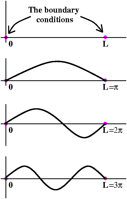For many students, Problem #15 of section 3.5 was the first boundary value problem they had seen. ODE's usually have many solutions. Picking out solutions with initial values is simplest: "Superman leaps from a 20 story tall building with a velocity of 20,000 furlongs per fortnight ..." But that's not the way natural problems are always stated. Superman may leap from a building, but he might want to be a specifc place at some specific later time.

With simple hypotheses, initial value problems have solutions defined for at least for short intervals of time from their starting point. Boundary value problems may not have solutions. Here's the most famous boundary value problem (and this is relevant to 421 because we'll see it again when we consider Fourier series):
We want to find y so that y''+y=0 and y(0)=0 and y(L)=0.
L is a positive number. Here we're looking for a function satisfying two "separated" conditions. Of course, there is always one solution for this problem, the function which is always 0. That's not too interesting, so we will look for solutions which are not always 0.

Take the Laplace transform. Then s²Y(s)-sy(0)-y'(0)+Y(s)=0. I do know that y(0) should be 0 but I don't know any simple way to use the information about y(L) in the Laplace transform. I'll call y'(0), K, and hope that the one free variable K will allow me to satisfy y(L)=0 later (something like that essentially happened in the homework problem). So let's take the inverse Laplace transform. Since Y(s)=K/(s²+1), then y(t)=K sin(t). We want y(L)=0, or K sin(L)=0. One way of achieving that is with K=0 but then the whole solution, y(t), is always 0, and this isn't the type of solution we want for our boundary value problem. But then sin(L) must be 0. This can only happen if L is a multiple of Pi: Pi, 2Pi, 3Pi, ... So there is no solution for other L's! This setup models "small" vibrations of a string which is fixed at both ends. So we've seen that there will be a "discrete" collection of solutions, corresponding (later in the course!) to the fundamental tone of the string and all of its overtones. The horizontal scales differ in the graphs -- a slightly different equation will be used to analyze vibrations.

H and delta
I asked how H, the Heaviside function, and delta, the Dirac delta function, were related. In the operational calculus we have been studying, it turns out that H' should be delta. So if we have a change in something which jumps, the derivative of this change should be delta (this is relevant to the salt problem I discussed last time).

Why should H' be delta? Well, certainly the ordinary derivative of H should be zero away from 0, because the graph is really flat there. What happens at 0? H jumps a whole unit. Since it is a unit jump, then the derivative should be a unit jump. Sigh. If this doesn't convince you, let me try another argument.

Let's approximate H by a nice smooth function, whose derivative always exists. Call the approximation W. Here's a picture of one possible W. This W follows H quite closely. In fact, it differs from H in only a short interval around 0. There (since W is increasing) W' is positive. It is sort of a lump. What is the area under this lump? Well, I'd like _-infty^inftyW'(t) dt. This is the same as _-26³⁵W'(t) dt b ecause W'(t) is 0 in lots of places. I can evaluate this with the Fundamental Theorem of Calculus. It is W(t)|_t=-26^t=35=W(35)-W(-26) which is 1-0 or 1. So if W is a really really good approximation to H then W' seems like an increasingly localized (around 0) "lump" of total mass 1. W'(t) has the important "filtering property", that, as the approximation W of H gets better,the integral _-infty^inftyW'(t)f(t) dt-->f(0), so W' behaves just like the delta function. That's why the rate of change (!!) of H is supposed to be delta. There are also some other reasonable arguments, but I hope you will believe this one.

This could even help us define the derivative of various piecewise functions where there are jumps. Each jump would correspond to an appropriate Dirac delta function, localized around the jump, that is, (Const)delta(t-[Jump]), where Const is the vertical height of the jump.

I wanted to add a few more formulas to our table of Laplace transforms.

An integral formula
What is the Laplace transform of ₀^inftyf(t) dt? Well, this simple antiderivative is really a convolution of the function f(t) with the constant function, 1. We know that the Laplace transform of 1 is 1/s and we call the Laplace transform of f(t), F(s). Therefore,
the Laplace transform of ₀^inftyf(t) dt is F(s)/s. Applications of this formula are in the convolution section and what follows that section.
Note If f(t) is the delta function, than F(s) is 1, so the Laplace transform of the integral of the delta function is 1/s, which means that f(t) would have to be H(t). This might reinforce the previous discussion.

Another weird formula
We know that the Laplace transform of f is ₀^inftye^-stf(t) dt. If we d/ds this formula, and keep very careful track of all the variables, we notice that the only place s appears is in the exponential. And d/ds of e^-st is -t e^-st. Therefore
(d/ds)₀^inftye^-stf(t) dt=-₀^inftye^-st(t·f(t)) dt.
To get the Laplace transform of t multiplying a function, take the function's Laplace transform and differentiate it and negate (multiply by -1) the result. Amazing! (Or irritating). So multiplying f(t) by tⁿ on the Laplace transform side is: adjust the sign (multiply by (-1)ⁿ) and differentiate F(s) n times with respect to s.

A textbook example
I bravely tried a textbook example, #9 from section 3.7. here it is:
"Use the Laplace transform to solve ... y''-8ty'+16y=3; y(0)=0, y'(0)=0."
So I obediently took the Laplace tranform of both sides. The right-hand side gives me 3/s. On the left, the first term is s²Y(s)+{Initial condition terms), and the initial condition terms are both 0. The third term on the left side gives 16Y(s). It is the middle term which is interesting and new here. The paragraph on "another weird formula" above allows us to identify the Laplace transform of -8ty'. First, "peel off" the -8. What's the Laplace transform of ty'? It is -d/ds of the Laplace transform of y'(t). But that is sY(s)-y(0). Since y(0) is 0, we d/ds the term sY(s) and get (product rule!) Y(s)+sY'(s). Now multiply by the - sign from the weird formula, and then multiply by -8 from the original statement. The result is the Laplace transformed equation:
s²Y(s)+8Y(s)+8sY'(s)+16Y(s)=3/s.

The result here is a differential equation involving Y(s), and not an algebraic equation for Y(s) as we had before. Let me rewrite this as you may have seen it in a previous ODE course:
8sY'(s)+(s²+24)Y(s)=3/s.
Now let me divide by 8s (carefully doing the algebra!) and think a bit:
Y'(s)+[(s/8)+(3/s)]Y(s)=3/(8s²).
This linear first-order ODED for Y(s) can be solved (I hope!) with an integrating factor. What is that? Well, if we look at the derivative of e^A(s)Y(s), it will be e^A(s)Y(s)+A'(s)e^A(s)Y(s) (yes, you should at least vaguely recall this trick!). So we want to match patterns with the left-hand side of the equation above, Y'(s)+[(s/8)+(3/s)]Y(s) , after we multiply it by e^A(s). Well, the pattern matching yields A'(s)=[(s/8)+(3/s)], and therefore A(s)=(1/(16))s²+3ln(s) (yes, I admit I got this wrong in class!). So we should multiply the equation by e^{(1/(16))s2+3ln(s)}. Then the left-hand side becomes the derivative of e^{(1/(16))s2+3ln(s)}Y(s). That's the whole purpose of the integrating factor trick: multiply by an exponential term and make the left-hand side a derivative. What about the right-hand side? It is e^{(1/(16))s2+3ln(s)}[3/(8s²)]. I would like to antidifferentiate this, also. At first it looks like junk. But, wow, continue looking:
e^{(1/(16))s2+3ln(s)}[3/(8s²)]=e^(1/(16))s2·e^3ln(s)[3/(8s²)]=e^(1/(16))s2s³[3/(8s²)]=e^(1/(16))s2(3/8)s
We happen to have exactly a combination of powers and exponentials so that we can exactly find an indefinite integral. It would be 3e^(1/(16))s2. So our differential equation is now:
The derivative of e^{(1/(16))s2+3ln(s)}Y(s) equals the derivative of 3e^(1/(16))s2.
Mr. Ivanov asked me why I took the constant of integration to be 0. After not much thought, I replied, "Because it's easier that way," which is maybe not a very good answer.

Now we have e^{(1/(16))s2+3ln(s)}Y(s)=3e^(1/(16))s2 so that e^3ln(s)Y(s)=3 and (after more exponential juggling!) we get Y(s)=3/s³ and we read the Laplace transform table backwards (Lerch's Theorem) to get y(t)=(3/2)t².

I then checked this answer by substituting it into the original equation and verifying that it solved both the equation and the stated initial conditions. It did.

Doing this example in class took, I was told, 17 minutes. I felt I went very fast. I had rehearsed, of course. It may make students feel better to know that typesetting this example has taken more than 45 minutes (!). What have I (we?) learned? Well, you can use Laplace transforms to solve ODE's which don't have constant coefficients. But, more than that, as I worked through this example, again and again, at least three times, I was struck by the prearranged nature and the manufactured coincidences which allowed us to solve this equation with a simple formula. How likely are such things to occur with either a random (!) example or a "real-world" example?

I confessed that I could not solve problem #1 in section 3.7 as stated and requested help.

A neat computation

I wanted to do something nice, nearly the end of our time with Laplace. A function which arises in some aspects of engineering is sin(t)/t. In fact, the function of x determined by 0x[(sin(t)/t] dt is known as the "sine integral function", Si(x), and has been tabulated and is one of the functions known to, say, Maple. The behavior of sin(t)/t as t-->0 is only apparently bad, because L'Hopital's rule will tell you quickly that the "correct" value of sin(t)/t at 0 is 1. If you graph sin(t)/t for positive t, you will see that the bumps alternate in sign and the geometric area in each bump decreases (because of the t in the denominator). Therefore (Alternating Series Test) the total area from 0 to infinity of sin(t)/t is finite. What is it? Here is a Laplace transform way of finding this area. I do know other methods to get this area, but this is certainly the shortest. Suppose f(t)=sin(t)/t. Then t f(t) is sin(t) whose Laplace transform is 1/(s2+1). But the weird fact above implies that the Laplace transform of t f(t) is -d/ds of the Laplace transform of f(t). So d/ds(F(s))=-1/(s2+1). But I know that the antiderivative of -1/(s2+1) is -arctan(s)+C. Here I will keep track of C. In fact, I know that as s-->infty, the function arctan(s)+C should approach 0, because Laplace transforms of nice functions do -->0 as s-->infty (since e-st shrinks down so quickly for large s). But what value of C will cause -arctan(s)+C to approach 0 as s-->infty? I recall that arctan(s)-->Pi/2 when s gets large. Therefore the choice should be C=Pi/2, and the Laplace transform of sin(t)/t is -arctan(s)+Pi/2. Consider though, that this is supposed to be equal to 0inftye-st[sin(t)/t] dt. When s=0, this is 0inftysin(t)/t dt but when s=0, -arctan(s)+Pi/2 is Pi/2. So Pi/2 must be the value of that improper integral, the total signed area "under" sin(t)/t from t=0 to t=infinity. The computation I showed you is not obvious. I can't (no one can!) find an antiderivative of sin(t)/t in terms of well-known functions, so to me it seems remarkable that we're able to compute the area exactly by any method.

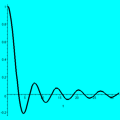
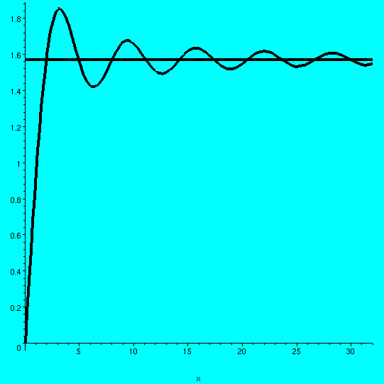
A graph of sin(t)/t on [0,32]   A graph of Si(t) and a horizontal line at Pi/2 on [0,32]

Conclusions on the Laplace transform
Here are some of my feelings about the Laplace transform.
Good stuff

• Treats some "rough" functions (Dirac, Heaviside) which might be useful in modeling real-world phenomena equally with a collection of "ordinary" functions defined by formulas, including polynomials, some trig functions, and some exponential functions.
• Unifies the initial conditions with the differential equations in solving initial value problems.
• It is another tool to keep in mind when analyzing and solving (?) ODE's.

• If the function doesn't appear on a Laplace function table, and if you can't deduce it using, say, the shift theorems and other results, and if a tool like Maple can't either, then you might find difficulty in taking the inverse Laplace transform ("Bromwich's integral" is an improper complex line integral).

Award certificates were distributed to students showing meritorious behavior (they came to class) during the Laplace transform part of the course.

We will next study linear algebra. Please look at the newly expanded and complete syllabus for the course.

The QotD was: what is the Laplace transform of the function which is t from 0 to 2, and is then t²? This is t+H(t-2)(t-t). We rewrite t²-t in terms of t-2: t²-t=([t-2]+2)²-t=(t-2)²+4(t-2)+4-t=(t-2)²+4(t-2)+2+(2-t)=(t-2)²+4(t-2)-(t-2)+2=(t-2)²+3(t-2)+2. So the Laplace transform of H(t-2)(t-t) will be e^-2s(2/s³+3/s²+2/s) and then we must add 1/s², the Laplace transform of t.
So the answer is e^-2s(2/s³+3/s²+2/s)+1/s².

A salt tank contains 100 liters of pure water at time t=0 when water begins flowing into the tank at 2 liters per second. The incoming liquid contains 1/2 kg of salt per liter. The well stirred liquid lows out of the tank at 2 liters per second. Model the situation with a first order ODE and find the amount of the salt in the tank at any time.

I remarked that I expected students had modeled and solved such problems a number of times in various courses, and certainly in Math 244. I did change my initial choice of name for the amount of salt, s, since continuing with that led to expressions like sS(s) on the Laplace transform side, and I make enough errors already!

Let y(t) be the kgs of salt in the tank at time t in seconds. We are given information about how y is changing. Indeed, y(t) is increasing by (1/2)2 kg/sec (mixture coming in) and decreasing by (2/100)y(t), the part of the salt in the tank at time t leaving each second. So we have:
y'(t)=1-(1/50)y(t) and y(0)=0 since there is initially no salt in the tank.
Mr. Marchitello described what the solutions should look like: a curve starting at the origin, concave down, increasing, and asymptotic to y=50. In the long term, we expect about 50 kgs of salt in the tank. This is easy to solve by a variety of methods, but in 421 we should use Laplace transforms: so let's look at the Laplace transform of the equation. We get sY(s)-y(0)=(1/s)-(1/50)Y(s). Use y(0)=0 and solve for Y(s). The result is Y(s)=1/[s(s+(1/50))]. This splits by partial fractions of some guesses to Y(s)=50[(1/s)-(1/(s+(1/50)))]. It is easy to find the inverse Laplace transform and write y(t)=50(1-e^-(1/50)t) which is certainly the expected solution.

Now the problem becomes more interesting.

Suppose that at time t=20 seconds 5 kgs of salt is instantaneously dropped into the tank. Modify the ODE from the previous part of the problem and solve it. Plot the solution to make sure it is sensible.

Now things are slightly more interesting. First I asked students what would likely happen. They remarked that they expected a jump in y(t) at time 20 of 5, but that then the solution would continue to go asymptotically to 50 when t is large. How should the ODE be modified to reflect the new chunk of salt? After some discussion, we decided it should be
y'(t)=1-(1/50)y(t)+5delta(t-20) and y(0)=0.
The delta function at t=20 represents the "instantaneous" change in y(t) at time 20, an immediate impulsive (?) increase in the amount of salt present.

Several substantive comments were made by students about this model. One, by Mr. Ivanov, was that real salt would probably drop in a clump to the bottom of the tank and would be dissolved at some real rate, not "instantaneously", by the mixing fluid. I think he is correct, more or less. But all of this modeling is more or less a first approximation (and an exercise in using Laplace transforms!).

Mr. Wilson had a different question after class. He asked why the delta function was appropriate in the equation for dy/dt. Certainly the salt (as a function of time) would have a Heaviside function added, but why does that turn into a delta function in the derivative? I think his question is a good one, which will be the first topic I'll try to discuss in the next class. But, briefly, a Heaviside function is mostly flat, so, mostly, its derivative should be 0. But it does have an instant (?!) jump of one unit, and the change represented by that jump is modeled by an appropriate delta function. That statement needs more justification, which I will try to give.

Back to solving y'(t)=1-(1/50)y(t)+5delta(t-20) and y(0)=0. Take the Laplace transform as before, and use the initial condition as before. The result is now sY(s)-y(0)=(1/s)-(1/50)Y(s)+5e-20s from which we get Y(s)=50[(1/s)-(1/(s+(1/50)))]+5[e-20s/(s+(1/50))] which has inverse Laplace transform y(t)=50(1-e-(1/50)t)-5H(t-20)e-(1/50)(t-20). Of course I wanted to check my answer, so I used Maple. Here is the command line and here is Maple's response: invlaplace(1/(s*(s+(1/50))) +5*exp(-20*s)/(s+(1/50)),s,t); 100*exp(-1/100*t)*sinh(1/100*t)+ 5*Heaviside(t-20)*exp(-1/50*t+2/5) Well, Maple multiplied 1/50 by 20 to get 2/5. Slightly more interesting is the sinh (hyperbolic sine, pronounced "cinch") part. Apparently users of Maple are expected to know that sinh(w)=(ew-e-w)/2. If you know that, then you can see that Maple's answer is equal to ours. You probably should also know about hyperbolic cosine, cosh, (pronounced "cosh") which is defined by cosh(w)=(ew+e-w)/2. Anyway, our answer does agree with Maple's. I also asked Maple to draw the solution, and the graph is to the right, with a dotted line at y=50. The solution is plotted on the interval [0,150]. A jump is visible at 20, and the asymptotic behavior is also displayed. In class I thought that the jump would have put the salt above the equilibrium amount, and there would be decrease afterwards. This does happen if you dump in 20 kgs of salt in at t=100, say, and then plot the solution from 0 to 250. The second picture shows that solution.

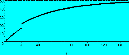
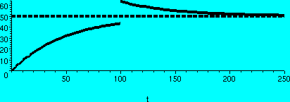
5 kgs in at 20 secs and t in [0,150].   20 kgs in at 100 secs and t in [0,250].

2. Resonances revisited
I went back to the problem I discussed during the last lecture, which was "kicking" an ideal spring periodically. So the model is y''+y=a sum of delta functions. If the delta functions are spaced 2Pi apart, then one can explicitly solve and see by evaluating at specific points that the function is unbounded (there is "resonance") and that some aspect of the model (or of reality!) fails.

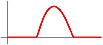I then asked students to think about the physical motion of such a spring which is kicked every Pi, so that y''+y=the sum of delta(t-j Pi) as j goes from 1 to infinity. I asked people to guess what the physical motion of the spring would be. After some silence, Mr. Morgan waved a finger to illustrate the beginning of a graph which looked like what's displayed. I said that was correct, and solution of the model shows exactly such behavior. There didn't seem to be much agreement, so I remarked that I would make this a homework problem.

Now what happens when the kicking occurs at positive integer intervals, so that we have y''+y=delta(t-1)+delta(t-2)+delta(t-3)+delta(t-4)+... Initially the spring is unmoving: y(0)=0 and y'(0)=0. The Laplace transform then gives (s²+1)Y(s)=e^-s+e^-2s+e^-3s+e^-4s+... The right-hand side is a geometric series (Google has about 670,000 pages with geometric series on them, and the first ideas of geometric series are usually taught in U.S. high schools and sometimes junior high schools). The first term is e^-s (called "a") and the constant ratio between successive terms is also e^-s (called "r"). The sum of a+ar+ar²+ar³+... is a/(1-r), so the sum of the right-hand side of the Laplace transformed equation is e^-s/(1-e^-s). Therefore Y(s)=(1/(s²+1))·(e^-s/(1-e^-s)). My guess is there is no huge reinforcement of amplitudes, so the inverse Laplace transform of (1/(s²+1))·(e^-s/(1-e^-s)) should be bounded. I have a picture of this inverse transform in the interval [0,30]. The picture is weird and wiggly. It does not convince me that that the function will be bounded from t=0 to, say, t=10,000. This sort of question might well come up in practice. Using a computer to plot something so delicate out to 10,000 is difficult. I tried to find an explicit inverse Laplace transform in our tables, and then I used Maple. I could not find any help. What could an engineer do now?

3. Some systems
The next section in the text uses the Laplace transform to solve some simple linear systems. I was uninspired, and did problem #2 in section 3.6. I hope I solved it correctly. Here it is:
2x'-3y+y'=0
x'+y'=t
with initial conditions x(0)=0 and y(0)=0. I asked people if they had done such problems in 244, and got mumbled replies that seemed to include, "Yeah, maybe, with linear algebra or something." The enthusiasm was shrinking like exponential decay. We Laplace transformed the equations, taking advantage of the initial conditions.
2sX(s)-2x(0)-3Y(s)+sY(s)+y(0)=0
sX(s)-x(0)+sY(s)-y(0)=1/s²
so that 2sX(s)-3Y(s)+sY(s)=0 and sX(s)+sY(s)=1/s²
If we multiply the second equation by 2 and subtract it from the first, we get -(s+3)Y(s)=-2/s² so that Y(s)=2/[s²(s+3)]=A/s+B/s²+C/(s+3) (partial fractions) and so 2=As(s+3)+B(s+3)+Cs². The magic number s=0 tells me that B=2/3 and s=-3 tells me that C=2/9. I could then work on getting A, but we know already because of our huge Laplace transform table that y(t) must be A+Bt+Ce^-3t so that y(0) will be A+C and since y(0)=0 and C=2/9 then A must be -2/9. This cute idea came from Mr. Wilson. Therefore y(t)=(-2/9)+(2/3)t+(2/9)e^-3t. Maple packages this answer as -2/3*t-4/9*exp(-3/2*t)*sinh(3/2*t) which does work out to be the same as ours.

What about X(s)? Since sX(s)+sY(s)=1/s² we know that X(s)+Y(s)=1/s³ and X(s)=1/s³-Y(s)=1/s³+known stuff. Therefore x(t)=(t²/2)-[(-2/9)+(2/3)t+(2/9)e^3t].

I checked with Maple and these formulas do satisfy the original equations.

I began to run out of energy, especially since I had left one page of my notes (two sides!) back in my office. I don't have this stuff memorized, I don't know it well enough, and ... well, those students who did not attend were missing a mediocre experience at best. Even the QotD (which I had prepared!) was screwed up. I tried in invent a system "on the fly" which people could solve by Laplace transforms. I should have settled for asking that people translate the system via Laplace transforms and then solve for one Laplace variable, such as Y(s). The system I wrote was:
x'+x+y'=delta(t-1)
4x'+2y+y'=1
with the initial conditions x(0)=0 and y(0)=0 to make it easy, of course.
The Laplace transform is:
sX(s)+X(s)+sY(s)=e^-s
4sX(s)+2Y(s)+sY(s)=1/s
after using the initial conditions. This becomes two linear equations in X(s) and Y(s): (s+1)X(s)+sY(s)=e^-s
4sX(s)+(s+2)Y(s)=1/s
Multiply the first equation by 4s and the second equation by (s+1):
4s(s+1)X(s)+4s²Y(s)=4s e^-s
(s+1)4sX(s)+(s+1)(s+2)Y(s)=(s+1)/s
Subtract the second equation from the first equation:
[4s²-(s+1)(s+2)]Y(s)=4s e^-s-(s+1)/s
and divide:
Y(s)=[4s e^-s-(s+1)/s]/[4s²-(s+1)(s+2)]
This is fairly horrible and I am embarrassed. It is much too hard for me to solve "by hand". Maple does it, of course, in about a tenth of a second. That's a very large chunk of time -- Maple takes less than a thousandth of a second to find the exact sum of the fifth powers of the first thousand integers! This was a very poor QotD.

The homework is: finish reading Chapter 3. Please hand in 3.5: 3, 15, 19 and 3.6: 9. Please solve the equation y''+y=the sum of delta(t-j Pi) as j goes from 1 to infinity. subject to the initial conditions y(0)=0 and y'(0)=0 and graph your solution! You may verify that Mr. Morgan's guess is essentially correct, but supply more of a graph and more coordinates on the graph!
Hint for 3.5 #15

Early Warning We should have a test fairly soon: about ten days or two weeks. Please let me know what exams you have in your major courses, and I will try to avoid close conflicts as much as I can. Tuesday will be the last lecture on Laplace stuff, and then we will move on to master Linear Algebra.

Oliver Heaviside remarked: "Should I refuse a good dinner simply because I do not understand the process of digestion?" (This refers to the lack of rigorous mathematical foundation for much of his work.) Here is another quote from Heaviside: "Mathematics is an experimental science, and definitions do not come first, but later on." I believe I agree with this statement. Heaviside was an engineer. One of his accomplishments was creating an "operational calculus" for solving differential equations. We have been studying his methods,and will conclude today by introducing a "function" named for Dirac. Dirac, a Nobel prize-winning mathematical physicist, worked on quantum mechanics and relativity. Here is an interesting quote from Dirac: "I consider that I understand an equation when I can predict the properties of its solutions, without actually solving it." A contemporary interview with Dirac may give some idea of his personality. As you will see, the Dirac function isn't a function (!) so indeed there are difficulties.

Here is a nice essay about the delta function and Laplace transforms.

And now (finally!) to the class
I began this lecture by finishing the remarks about convolution: how approximate integration of the convolution integral in the problem I analyzed last time makes real-world sense, and is computationally very feasible. (Please see the discussion at the end of the previous lecture.)

Here are some properties of convolution which can be useful in computations.

Convolution facts
Commutativity	f * g = g * f
Associativity	(f * g) * h = f * (g * h)
Linearity in each variable	(f1+f2) * g = (f1 * g) + (f2 * g) f * (g1+g2) = (f * g1) + (f * g2)

Then I did Problem #20 in section 3.4, which is: find f(t) if you know that f(t)=-1+t-2₀^tf(t-tau)sin(tau) dtau. Of course we recognize the integral as a convolution (this is a problem in a textbook, darn it!). If we take the Laplace transform of both sides, then the equation becomes F(s)=-(1/s)+(1/s²)-2(F(s)/(s²+1)). The convolution turns into multiplication. We then solve for F(s) and get (after a bit of algebra) F(s)=[-(1/s)+(1/s²)]·[(s²+1)/(s²+3)]. We can use partial fractions to split this up into (A/s)+(B/s²)+(Cs+D)/(s²+3). As direct wrote in the quote above, maybe we can try to predict the solution. In fact, with the help of a table of transforms, I can read off that f(t) will be A+Bt+C cos(sqrt(3)t)+(D/sqrt(3))sin(sqrt(3)t). I tried this by hand, and then had Maple use invlaplace on it. Maple reported that the solution was -(2/3)cos(sqrt(3)t)+(2/9)sqrt(3)sin(sqrt(3)t)+(t/3)-(1/3). This has the predicted form, so I was sort of happy. But I then went on, and used Maple to check that this function actually satisfied the integral equation I started with.; For a human being, this check would have been a rather irritating computation, but for Maple the confirmation was rapid and easy

An impulse and limits of impulses
We can think of an impulsive "kick" as mechanically sort of the limit of a square wave. Let me show you how Heaviside might have presented this. The total area under a wave is the amount of the impulse. So if I want to somehow keep this constant but would like to shrink the time in which the energy is transferred, then I need to make the amplitude higher. So what I did was create a square wave which was 0 for x<0 and for x>epsilon. If I want the total area to still be 1, then inside the interval [0,epsilon] the function should be 1/epsilon. The graph then is a rectangular block whose area is epsilon·1/epsilon=1. What's the Laplace transform of this function? We can do a direct computation, as we already have several times with such functions. Or, better in this course, we can express the function with Heaviside functions and use our tables. Then the function is (1/epsilon)H(t)-(1/epsilon)H(t-epsilon). The Laplace transform of this (using results from the last lecture) is (1/epsilon)(1/s)-(1/epsilon)e^-epsilon s(1/s). It takes some effort not to rewrite this, and why resist: (1/s)[(1-e^-epsilon s)/epsilon]. What happens to the impulse as epsilon-->0? This is a limit, and I'll plug in epsilon=0. The result is 0/0 (much better than 56/0, actually!). So I can try l'Hopital's rule, and differentiate the top and bottom with respect to epsilon. Although each step in all this is easy (almost trivial, maybe) the opportunity for confusion is large, because there always seem to be extra variables present. In this case, the result of d/depsilon top and bottom is (1/s)[(--s e^-epsilon s)/1]. Now if epsilon-->0, the result is s/s or 1. The Laplace transform of this limiting impulse is 1.

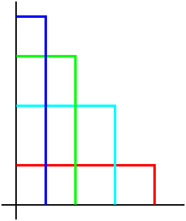
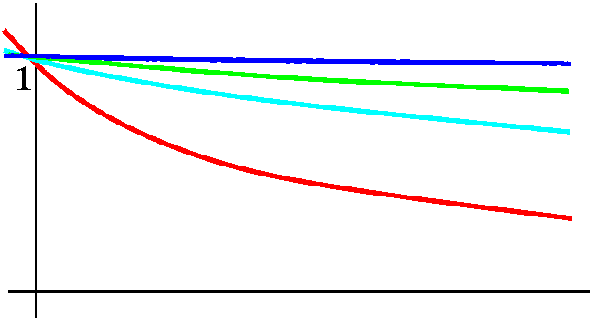
The picture below is an almost poetic (!) attempt to show you what's happening. As the impulses get narrower and higher (but all with area=0) the corresponding Laplace transforms are exponentials which -->1.

A sequence of impulses	Their Laplace transforms

A comment
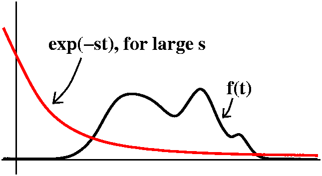Something a bit startling has occurred. When I began discussing Laplace transforms, I declared that if f(t) were some sort of blobby function, then the Laplace transform would be gotten by integrating the product of f(t) with e^-st. And if you consider the picture, when s gets really really really large, then the exponential dies down very very very fast, and so the Laplace transform should -->0 as s-->infty. But we seem now to have a Laplace transform (the limit of the square waves) which is is 1, so something seems wrong. This is more or less the position of academic mathematicians when Heaviside was presenting his methods. In fact, almost half a century passed before the ideas of Heaviside would become part of rigorous mathematical thought. His feeling, and that of many engineers and physicists, was that, my goodness, the methods work, so use them and don't worry too much.

I then tried to analyze some more properties of this limiting square wave. I said suppose we take a positive integer n and define f_n by making it n on the interval [0,1/n] and 0 elsewhere. This is a sequential version of the epsilon impulse. Now I asked: what is lim_{n-->infty -36}⁴⁵f_n(x) dx? This may look formidable but it is easy, because the box is inside the interval [-36,45] and the box's area is always 1, so the limit is 1. What about lim_{n-->infty 23}⁵⁸f_n dx? Here again the limit is easy, because inside the interval [23,58] all the f_n's have value 0. The limit is 0.

Now let's try a more sophisticated limit. Suppose g(x)=e^x+7+6x². What is lim_{n-->infty -5}¹⁸f_n(x)g(x) dx? Of course please realize that -5 and 18 are mostly irrelevant. All that really matters is that the x's where f_n(x) is not 0 are inside [-5,18]. If you think carefully about the picture, you can see that the integral is narrowing down and weighting more and more the value g(0). If you want some better "intuition", here: the integral from 0 to 1/n (that's where f_n is not 0) of g(x) is equal to g(some number between 0 and 1/n) multiplied by the length of the interval of integration, which is 1/n. So _-5¹⁸f_n(x)g(x) dx = ₀^1/nf_n(x)g(x) dx = n₀^1/ng(x) dx. The last equality is correct because the function f_n is n inside the interval [0,1/n]. But ₀^1/ng(x) dx =g(some number in [0,1/n])·(1/n) by Mean Value Theorem for Integrals. The 1/n and n cancel, so that ₀^1/nf_n(x)g(x) dx = g(some number between 0 and 1/n). Since our g(x)=e^x+7+6x² is continuous, g's values near 0 approach g(0) which is e⁰+7=8. Therefore lim_n-->infty0^1/nf_n(x)g(x) dx = g(0) = 8.

What Mr. Heaviside then did, which upset the academics, was define the delta function at 0, delta(t), (now usually called the Dirac delta function) by lim_n-->inftyf_n(x). This is more a "function" than a function. Why is this? The value of delta(t) for t not equal to 0 is surely 0. But the integral of t from -infty to +infty is "surely" 1 (well, I want it to have integral 1). If delta(t) were an ordinary function, it would need a value at 0, and maybe the value at 0 would have to be infinity? (And I don't understand infinity very well!)

Behavior of the delta "function"
If t is not 0, then delta(t)=0 The Laplace transform of delta(t) is the constant function 1. If g is continuous, then -infty+inftydelta(t)·g(t) dt=g(0).

We can translate the delta function, just as we translated the Heaviside function. What does delta(t-5) do? The center of interest is then where t-5 is 0, or where t=5. That means, for example, that _-infty^inftydelta(t-5)·g(t) dt must be g(5) if g is continuous at 5. Etc.

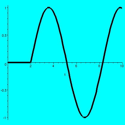So it is time to solve a differential equation. Let's try something simple (of course!): y''+y=delta(t-2) with the initial condition y(0)=0 and y'(0)=0. So this is a vibrating spring with no damping initially unmoving and in equilibrium, which we kick at t=2. Let's take the Laplace transform. The left-hand side is easy because all the complicated stuff drops out due to the initial conditions. We get (s²+1)Y(s). The right-hand side is e^-2s1 (the "1" is the Laplace transform of the delta function and the e^-2s is because we have shifted by 2 in the time variable). Then Y(s)=(e^-2s)/(s²+1). We transform back, noting that the exponential now makes "everything" start at 2: y(t)=H(t-2)sin(t-2). Here is the entire dialog of a Maple session to compute the solution, and then produce the graph shown.

with(inttrans):
laplace(Dirac(t-2),t,s);
                              exp(-2 s)
invlaplace(exp(-2*s)/(s^2+1),s,t);
                     Heaviside(t - 2) sin(t - 2)
plot(%,t=0..10,thickness=5,color=black);

BOOM! BOOM!! BOOM!!!
Chris Stucchio, a mathematics graduate student here, suggested the following. There was once a proposal to propel spaceships by exploding atom bombs in back of them and using the push from the explosions to move the spaceships. We are not making this up! It was called Project Orion. Since from a real-time point of view, an atom bomb explosion is darn near an idealized delta impulse, I guess we could have analyzed the resulting motion. Instead, I was more modest.

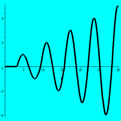
Resonance I think that Ms. Kohut suggested we try to "kick" the vibrating spring periodically. So I tried to analyze this equation: y''+y=delta(t-Pi)+delta(t-3Pi)+delta(t-5Pi)+delta(t-7Pi)+delta(t-9Pi)+... with initial conditions y(0)=0 and y'(0)=0. Now Laplace transform everything: (s2+1)Y(s)=e-(Pi)s+e-(3Pi)s+e-(5Pi)s+e(-7Pi)s+... and divide by s2+1 and transform back. The solution seems to be y(t)=H(t-Pi)sin(t-Pi)+H(t-3Pi)sin(t-3Pi)+H(t-5Pi)sin(t-5Pi)+H(t-7Pi)sin(t-7Pi)+... and I've shown a graph of this on the interval from t=0 to t=30. It certainly looks like the model must break down somewhere (Hooke's law not valid, spring breaks, etc.). Look at what happens at (1.5)Pi, (3.5)Pi, (5.5)Pi, etc. (y(t)'s values at those t's are 1, 2, 3, etc.). Be a bit careful, please. This is not a picture of "smooth motion". 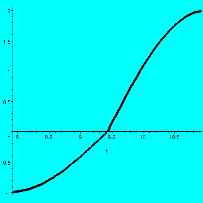There's kinky behavior (first derivative doesn't exist) at each odd multiple of Pi, corresponding to another delta function kick. Here is a closeup of the graph around 3Pi, so you can see the corner. I think the previous "bigger" view conceals this finer "structure". Challenge to the Mechanical Engineers Can you predict, without computation, what would happen if we kicked the spring every Pi instead of every 2Pi? I couldn't and the answer after I computed it was slightly surprising to me. Can you? Non-resonance? Remember that Pi is not rational: that is, it is not a quotient of integers. What if we "kick" the spring every integer? If you think things through, the kicks should not reinforce each other, and instead they should somehow distribute "around" the sine wave. Well, here is what I did. I tried to solve y''+y=delta(t-1)+delta(t-2)+delta(t-3)+... with y(0)=0 and y'(0)=0. 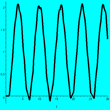Then Laplace transform tells me that Y(s)=[e-s+e-2s+e-3s+...]/(s2+1) and the inverse Laplace transform is H(t-1)sin(t-1)+H(t-2)sin(t-2)+H(t-3)sin(t-3)+H(t-4)sin(t-4)+... A picture is shown of the first thirty terms graphed on the interval [0,30]. The curve certainly seems very bounded, as if there is no reinforcement from resonance. I can't prove this. If we work on the Laplace transform some more, starting with Y(s)=[e-s+e-2s+e-3s+...]/(s2+1) the top is a geometric series with first term e-s and whose ratio is also e-s. So actually Y(s)=[1/(s2+1)]·[e-s/(1-e-s)]. This is a product, so y(t) would be a convolution of sine (whose Laplace transform is [1/(s2+1)]) and a function whose Laplace transform is e-s/(1-e-s)]. I don't know such a function, and, it seems, neither does Maple. So I can't go any further right now. Is it "clear" or "obvious" that the spring's motion is bounded to you? It isn't to me.

The QotD was: compute ₀¹⁰⁰[e^tcos(t)][5delta(t-Pi)+30delta(t-3Pi)] dt. Here I hoped that my explanation of the Dirac delta function was enough. I expected the answer would be (using linearity of the integral) 5·(the value of [e^tcos(t)] at t=Pi)+30·(the value of [e^tcos(t)] at t=3Pi). This is -5e^Pi-30e^3Pi. Most people seemed to get this correct (please note that cos(Pi) and cos(3Pi) are both -1, though!).

Continue reading the book.

Motivated by the fact that most students had gotten the previous QotD wrong, which is really not my aim, I decided to begin by asking pairs of students to "compute" Laplace transforms and inverse Laplace transforms. The computations would use information from the book and some examples I copied from Maple.

Information from the text (we also computed most of these in class) Function Laplace transform tn n!/sn+1 eat 1/(s-a) sin(at) a/(s2+a2) cos(at) s/(s2+a2)

Examples from Maple (using laplace and invlaplace in the package inttrans) Function Laplace transform t 1/s2 tet 1/(s-1)2 H(t-1) e-s/s H(t-2)[(t-2)et-2] e-2s/(s-1)2

It was my hope that the Maple examples would help students as they worked on the questions I gave them. Also students should be studying and reading the text. The text has formal statements of the needed theorems, and also has more examples.

#1
Mr. Cohen and Mr. Ivanov kindly tried to find the Laplace transform of sin(t)H(t-5). They wrote sin(t)=sin(t-5+5)=sin(t-5)cos(5)+cos(t-5)sin(5). Then they used linearity and the shifting theorem, which demands as input a function of the form H(t-a)f(t-a) and then has as output e^-asF(s). The result in this case is e^-5s(cos(5)/(s²+1)+sin(5)s/(s²+1).

#2
Here I gave the Laplace transform, e^-3s/(s²+4), and asked students (whose names I don't remember!) to find the function it "came from" (Lerch's Theorem, the inverse Laplace transform). The e^-3s in Y(s) indicates that y(t) will "begin" with H(t-3). The other part, looking in the first table above, gives something sort of about sin(2t). This isn't quite correct, because we need to fix the y(t) with a 1/2 to compensate for the missing "a" in the top of the Laplace transform of sin(at). But we must also shift the function by 3. Therefore the desired y(s) is H(t-3)sin(2(t-3)).

#3
Unknown students were confronted with Y(s)=s/[(s-3)(s-1)]. Yes, more complete tables would permit us to look up the answer, but can we get it from the information supplied? Yes, because we use partial fractions, and want to write s/[(s-3)(s-1)] as A/(s-3)+B/(s-1). This leads to A(s-1)+B(s-3)=s, so (s=3) A=3/2 and (s=1) B=-1/2, so that Y(s)=(3/2)/(s-3)+(-1/2)/(s-1) so (linearity) y(t) must be (2/3)e^3t+(-1/2)e^t.

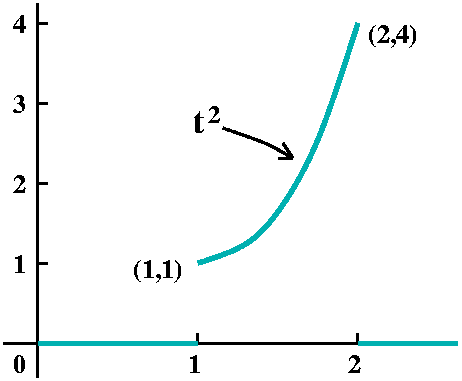#4
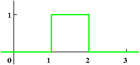
Here I gave graphical data. (The picture shown has differing units on the horizontal and vertical axes.) The function y(t) was 0 before t=1 and after t=2, and was t² between 1 and 2. As I mentioned in class, we could always compute the darn Laplace transform directly from the definition. But I am supposed to show you how to use the rather clever techniques developed (sometimes called the operational calculus). So in terms of these techniques, we turn t² on at t=1, and then turn it off at t=2. To turn it on, write H(t-1)t². Then we need to turn it off. This is H(t-2)(-t²).

We would like to find the Laplace transform of H(t-1)t²-H(t-2)(t²). But the shifting theorem demands that the function multiplied by H(t-1) be written in terms of t-1. Therefore write t²=(t-1+1)²=(t-1)²+2(t-1)+1. The Laplace transform of H(t-1)[(t-1)²+2(t-1)+1] is e^-s[2/s³+2/s²+1/s].

What about the other piece, -H(t-2)(t²)? Here we must write t² as a function of t-2: t²=(t-2+2)²=(t-2)²+4(t-2)+4. Therefore the Laplace transform of -H(t-2)(t²) is the same as the Laplace transform of -H(t-2)[(t-2)²+4(t-2)+4], and by shifting, this is -e^-2s[2/s³+4/s²+4/s].

Putting it all together, the result is
e^-s[2/s³+2/s²+1/s]-e^-2s[2/s³+4/s²+4/s]. I believe that the students who worked on this were Ms. Sirak and Mr. Wilson and I thank them.

#5
Again, graphical input: the function was composed of three pieces of straight lines. It was 0 until 5, then a line segment from (5,0) to (6,1), and then a horizontal "ray" at height 1. We can write this function as H(t-5)(line from (5,0) to (6,1))+H(t-6)(1-[line from (5,0) to (6,1)]). The line connecting (5,0) to (6,1) has slope 1 and goes through (5,0), so that its formula must be t-5. The function whose Laplace transform we want is therefore H(t-5)(t-5)+H(t-6)(1-[t-5])=H(t-5)(t-5)+H(t-6)(-t+6). Since (-t+6) is -(t-6) we can apply the shifting theorem "immediately"(well, almost). The desired Laplace transform is e^-5s(1/s²)-e^-6s(1/s²).

#6
The last problem was a monster, and Mr. Brynildsen and Mr. Elnaggar kindly attempted it. It was an inverse Laplace transform. I gave them Y(s)=e^-3s/[(s-8)²+4]. I wanted people to see that y(t) would have to"begin" at 3, so it would have H(t-3) (because of the e^-3s factor). The other part looks very much like sine.

Let's try to get the inverse Laplace transform of 1/[(s-8)²+4]. The translation by 8 is gotten by multiplying by e^8t. The other part, the inverse Laplace transform of 1/[s²+4], must be (1/2)sin(2t). So the inverse Laplace transform of [(s-8)²+4] is e^8t(1/2)sin(2t).

But [(s-8)²+4] is multiplied by e^-3s. That means we prefix the inverse transform by H(t-3) and put t-3 in for t in the other part of the inverse Laplace transform. Therefore the answer is H(t-3)[e^8(t-3)(1/2)sin(2(t-3))].

Well, I thought this would take 10 or 20 minutes, but we spent about an hour on it. I hope that the effort was useful. Certainly I made as many mistakes as all of the students together did, and I apologize for that.

The Shifting Theorems Function Laplace transform eatf(t) F(s-a) H(t-a)f(t-a) e-asF(s)

(The first result is the book's Theorem 3.7 and the second result is the book's Theorem 3.8, both from section 3.3.)

Today's topic: convolution and Laplace transform
Here's the definition. Suppose we have f(t) and g(t). Then the convolution of f with g, written as f_*g (that's a star or asterisk between f and g), is defined by the formula ₀^tf(t-tau)g(tau) dtau. I'm using tau for the Greek letter used in the text in this definition.

The first time I "see" a mathematical object, I immediately try to look at examples. Pure definitions rarely make sense to me. Simple examples are almost always the best. So let's try f(t)=t² and g(t)=t³. Then f_*g(t)= ₀^t(t-tau)²(tau)³ dtau. Expand so the integrand becomes t²tau³-2ttau⁴+tau⁵. Now antidifferentiate with respect to tau and substitute tau=t and subtract off the value when tau=0 (the contribution from the lower bound is 0 because we are dealing with monomials, but Warning! see what happens in the QotD computation below. The result of the antidifferentiation is t²(1/4)tau⁴-2t(1/5)tau⁵+(1/6)tau⁶ and therefore the whole convolution is (1/4)t⁶-(2/5)t⁶+(1/6)t⁶ which can be "simplified" to [(1/4)-(2/5)+(1/6]t⁶=[(15-24+10)t⁷=(1/60)t⁶.

This doesn't seem very helpful. Historically I believe that convolutions arose as a way to "package" solutions of differential equations, as I will try to show later. But what you could notice right now is the following:
    f(t)=t² has Laplace transform 2/s³.
    g(t)=t³ has Laplace transform 6/s⁴.
    (f_*g)(t)=(1/60)t⁶ has Laplace transform (1/60)(6!/s⁷).
Extensive computation (!) led us to 6!=720, and 720/60 is 12. If we match up the powers and the coefficients we see that 2/s³·6/s⁴=(12/s⁷). In this example the Laplace transform of f_*g is the product of the Laplace transform of f and the Laplace transform of g.

Here's an example I wanted to do in class. I want to compute explicitly f_*g where f(t)=e^t and g(t)=cos(t). Then f_*g(t)= ₀^te^t-taucos(tau) dtau. Since e^t-tau=e^te^-tau, we can take e^t out of the dtau integral. We need to find an antiderivative of e^-taucos(tau) dtau. We could integrate by parts twice, or use a trick we have already used once: cos(tau) is the real part of e^itau=cos(tau)+i sin(tau) so take the real part of the antiderivative of e^-taue^itau dtau=e^(-1+i)tau dtau. The antiderivative is [1/(-1+i)]e^(-1+i)tau. Notice that both of the endpoints of the convolution integral contribute here, because exponentials are 1 when their arguments are 0! Therefore we get [1/(-1+i)][e^(-1+i)t-1] and since (1/(-1+i)]=(-1-i)/2 and e^(-1+i)t is e^-t(cos(t)+i sin(t)), we have (1/2)(-1-i)(e^-t(cos(t)+i sin(t)-1). The real part is (1/2)(-e^-tcos(t)+e^-tsin(t)-1).

To get the convolution we still must multiply by the e^t factor we pulled out of the integral at the beginning. The convolution is therefore (1/2)(-e⁰cos(t)+e⁰sin(t)-e^t) which is (1/2)(-cos(t)+sint(t)-e^t). We can now look up the Laplace transform: (1/2)(-s/(s²+1)+1/(s²+1)-1/(s-1)).

The Laplace transform of e^t is 1/(s-1) and the Laplace transform of cos(t) is s/(s²+1). And (sigh, the details are too irritating to write) the product of these two functions is the transform of the convolution (again, partial fractions).

The following statement is true in general (see section 3.4):
      The Laplace transform of the convolution is the product of the Laplace transforms.

Here is a simple ODE with an initial condition: y'+3y=f(t) with y(0)=5. I first solved the "associated homogeneous equation", which wasn't too hard (a first-order constant coefficient ODE, after all): the solution is 5e^-3t. How does the input f(t) perturb or affect this simple solution? Well, let's take the Laplace transform of the whole equation. Here is what results: sY(s)-y(0)+3Y(s)=F(s). Put in the initial condition and solve for Y(s): Y(s)=F(s)/(s+3)+5/(s+3). Now take (try to take?) the inverse Laplace transform. The 5/(s+3) term leads to 5e^-3t. The other term must be the result of f's effect. Understand it this way: F(s)/(s+3) is the product of F(s) and 1/(s+3) so that its inverse Laplace transform is the convolution of f(t) and e^-3t. Write this out: ₀^tf(t-tau)e^-3(tau) dtau.

This is more profound and useful than might appear. The solution of y'+3y=f(t) with y(0)=5 is:     5e^3t + ₀^tf(t-tau)e^-3(tau) dtau.

Suppose that all we know about f(t) is some data:

Time 1 2 3 4 5 6 7 8 9 10 f(t) 36 28 17 5 4 4 2 1 -3 -5

How can we approximate, say, y(4)? y(4)=5e^3·4+₀⁴f(4-tau)e^-3(tau) dtau. I'll concentrate on trying to understand the integral term. We only know the data points at integer intervals. Approximate the integral by a Riemann sum using the left-hand endpoints as sample points. Therefore the integral is approximated by f(4-0)e^-3·0+f(4-1)e^-3·1+f(4-2)e^-3·2+f(4-3)e^-3·3 which equals 5e^-3·0+17e^-3·1+28e^-3·2+36e^-3·3.

What would a similar approximation look like for t=8? It would be f(8-0)e^-3·0+ f(8-1)e^-3·1+ f(8-2)e^-3·2+ f(8-3)e^-3·3+ f(8-4)e^-3·4+ f(8-5)e^-3·5+ f(8-6)e^-3·6+ f(8-7)e^-3·7= 1e^-3·0+ 2e^-3·1+ 4e^-3·2+ 4e^-3·3+ 5e^-3·4+ 17e^-3·5+ 28e^-3·6+ 36e^-3·7.

The computation of such sums on many modern computers is not hard, because things can be done in parallel. (This is basically a dot product.) You can see (this equations describes decay!) that data which is older has a proportionally lower effect on the sum. In f(4), the number 36 is multiplied by e^-3·3. In f(8), it is multiplied by 36e^-3·7. Think about this. Much more can be done. The QotD was: if f(t)=e^7t and g(t)=e^3t, compute f_*g(t).

Using the definition

Using the convolution product formula

0te7(t-tau)e3(tau) dtau= e7t0te-4tau dtau. This is e7t(-1/4)e-4tau|tau=0tau=t which is e7t(-1/4)[e-4t-1]. Recall the Warning! above. You shouldn't forget the lower limit.

The Laplace transform of e7t is 1/(s-7) and the Laplace transform of e3t is 1/(s-3). The product of these functions is 1/[(s-7)(s-3)]. As Mr. Dupersoy observed, you can look up the inverse Laplace transform of this in the text's table in section 3.1. I would be lazy and split 1/[(s-7)(s-3)] with partial fractions into (1/4)/(s-7)+(-1/4)/(s-3). The inverse Laplace transform of this is (1/4)e7t-(1/4)e3t.

There is joy because the answers are the same.

Please read sections 3.3 and 3.4. Section 3.5 has one of the really startling ideas of all of twentieth century mathematics. Please hand in 3.3: 25, 27, and 3.4: 3, 13, 17.

Note
I have been given a grader for this course. I want to give the grader one collection of problems each week. Therefore only very exceptional circumstances will allow me to accept late homework for credit. (I will read it for correctness, if you wish!)

Rough check for arithmetic?
By analogy, look at, say, the computation of this product: (2,345,509)·(4,111,345). I think (Maple told me) that this product is 9,643,196,699,605. But what if I had designed my own program to handle multiplication of l-o-n-g integers or I used a calculator which might be damaged? If the result I got was 9,643 then I would know there was a computational error. Or if I got -78 I certainly know the result was wrong. So are there similar checks I can use for this Laplace transform answer?

Let's see: the tent lives on the interval from A to A+2. The Laplace transform multiplies that by e^-st and integrates dt. I surely know that if s-->infty, the result will go to 0 since the exponential function pushes down on the product as s gets larger and larger (that's because of the - sign in the exponent, of course.)

Rough check #0
(Sorry: I forgot to do this one in class.) As s-->infty, the Laplace transform of the tent should -->0. Well, the suspected answer is [e^-sA-2e^-s(A+1)+e^-s(A+2)]/s² and, indeed, if we keep A fixed and make s get very large positive, the s² on the bottom and, especially, the negative parts of the exponentials make the function -->0.

Rough check #1
What if we move the tent? Let's say we make A-->infty? What should happen? For each value of the Laplace transform we are multiplying by exponential decay, so as the tent moves further right, the transform should get smaller. (The vibration or the signal is going more futurewards, perhaps?) Well, the answer is [e^-sA-2e^-s(A+1)+e^-s(A+2)]/s² and as A-->infty (with s constant!) then (again, the minus sign in the exponentials) the Laplace transform does -->0: good!

Rough check #2
There is actually a specific value of the Laplace transform we can check. We are multiplying the tent by e^-st. If we make s=0, then the exponential is always 1, and we are integrating the tent itself: we are computing the area under the tent. But the tent is two triangles each with area 1/2, so the total area is 1. Our suspected answer is [e^-sA-2e^-s(A+1)+e^-s(A+2)]/s² so when s=0, this should be 1. Plug in s=0. The bottom is 0, bad! What about the top? As Ms. Sirak said, the top had better be 0 also (it is, because when s=0 the top is 1-2+1). Why did she say that? Of course! Because we must use L'Hopital's Rule to check the value at s=0 and the "0/0" condition should be verified before we compute (or else we may get a wrong answer). So let's d/ds the top and bottom of [e^-sA-2e^-s(A+1)+e^-s(A+2)]/s². The result (keep all the variables straight: differentiate with respect to s): [e^-sA(-A)-2e^-s(A+1)(-(A+1))+e^-s(A+2)(-(A+2))]/[2s]. Now try s=0. On the bottom, the result is again 0. What about the top? We get -A-2(-(A+1))-(A+2): oh, wonderful! all the A's cancel and all the constants cancel. We get 0. So, supported by a 0/0 result, we L'Hop again. So d/ds the top and bottom separately: [e^-sA(-A)²-2e^-s(A+1)(-(A+1))²+e^-s(A+2)(-(A+2))²]/[2]. Now the bottom is not 0 when s=0: it is 2. What about the top? Again, s=0 makes the exponentials all equal to 1. The top is (-A)²-2(-(A+1))²+(-(A+2))² and this works out to be A²-2(A²+2A+1)+A²+4A+4. The A²'s and the A's cancel, and we are left with 2. That's the top, so the result is 2/2=1 which is what we wanted.

That certainly seems like a lot of effort for a "rough check". Here is another way to do it: e^x is approximately 1+x+(1/2)x²... (the initial segment of the Taylor series for the exponential function centered at 0). Then [e^-sA-2e^-s(A+1)+e^-s(A+2)]/s² becomes 1+(-sA)+(1/2)(-sA)²...   -2[1+(-s(A+1))+(1/2)(-s(A+1))²...   1+(-s(A+2))+(1/2(-s(A+2))²...   If you work out the algebra, you'll get the same answer as we had above.

I'm trying to supply some "intuition" (?!) for these computations, whose details may seem rather elaborate.

"Now we may perhaps to begin?" (This is the last line in the novel Portnoy's Complaint by Philip Roth)
Today's topics

• Translations and their effect on the Laplace transform
• The Heaviside function

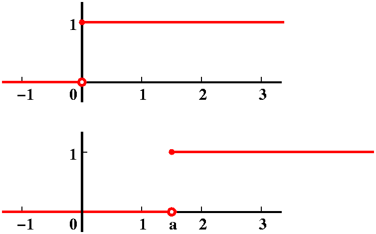Naturally I want to begin with the second topic. The Heaviside function is constant except for a jump of 1 at 0. It is the simplest piecewise continuous function. Here is a biography of Heaviside, whose life seems quite interesting. So H(t) is 1 if t>=0 and 0 if t<0. By the way, Heaviside is also what the Heaviside function is called both in Maple and Matlab. What's the Laplace transform of H? Notice, please, that the Laplace transform only "looks at" t>=0. For such t, the Heaviside function is same thing as 1, and 1's Laplace transform is 1/s. So the Laplace transform of H is 1/s. If a is a positive number, the function H(t-a) has a jump of 1 at a. Let's compute the Laplace transform of H(t-a). So we start with ₀^inftye^-stH(t-a) dt and this is _a^inftye^-st dt: remember to drop the part of the integral where H(t-a) is 0 and to keep (with 1) the other part of the integral. This integral is easy to compute. We get -e^-st/s|_t=a^t=infty. The infinity term disappears (exponential decrease) and the other part is e^-as/s. So if we translate the Heaviside function into the future, the Laplace transform which is 1/s gets multiplied by a compensating exponential, e^-as.

What happens to the future?
This is actually always true: translation of the vibration/signal y(t) into the future by a (that is, y(t-a)) will multiply the Laplace transform Y(s) by e^-as.

Example #1
Look at the bump we introduced in the first lecture: "a square wave: a function given by f(x)=0 for x<3 and for x>7 and f(x)=5 for x in [3,7]". This can be written using translates of the Heaviside function in a neat way. First, we don't need anything before t=3. At t=3, we want a jump of 5: 5H(t-3). Then we want to jump down at t=7: -5H(t-7). So this square wave can be written, symbolically, as 5H(t-3)-5H(t-7). We can compute the Laplace transform using linearity and the future idea above gives 5e^-3s/s-5e^-7s/s. I thank Mr. Obbayi for helping me with the correct variables in the exponentials here and in the other examples. I was told that this answer was the same as the answer we got by direct computation in the first lecture.

Example #2
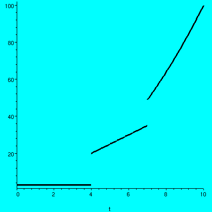
Here I tried a piecewise polynomial. The function f(t) was something like this: f(t) was 3 for t<4, and was 5t for t in the interval [4,7], and was t² for t>7. How can we write this using Heaviside functions? First f(t) is 3. Then we need to "switch on" 5t at t=4, so we need H(t-4)5t. And we want to similarly switch on t² at t=7, so we need H(t-7)t². But this so far isn't exactly correct. We need to turn off the previous signal when we introduce the new one. So this f(t) is actually 3+H(t-4)(5t-3)+H(t-7)(t²-5t). By the way, to the right is the result of the Maple command:
plot(3+Heaviside(t-4)*(5*t-3)+Heaviside(t-7)*(t^2-5*t), t=0..10, discont=true, color=black, thickness=3);
So you can see that Maple understands this language well.

Since f(t)=3+H(t-4)(5t-3)+H(t-7)(t²-5t), we can try to find the Laplace transform of f(t). Linearity again helps. We need to transform each piece. The Laplace transform of 3 is 3/s. What about H(t-4)(5t-3)? If this were a function of t-4 then its transform would be the transform of the function whose argument is t-4 then multiplied by e^-4s for the time shift. But, golly, 5t-3=5(t-4+4)-3=5(t-4)+17. Therefore H(t-4)(5t-3) is actually H(t-4)(5(t-4)+17). This is a time shift of the function H(w)(5w+23), whose Laplace transform is 5/s²+17/s (we had a small table of Laplace transforms on the board). Now multiply by the appropriate exponential factor, and the Laplace transform of H(t-4)(5t-3) is "just" e^-4s(5/s²+17/s). Now we need to handle the last chunk, which is H(t-7)(t²-5t). Now I would like to write t²-5t in terms of t-7. Do this with the following somewhat tedious algebra: t²-5t=(t-7  +7)²-5(t-7  +7). Therefore we have t²-5t=(t-7)²+14(t-4)+49-5(t-7)-35=(t-7)²+9(t-7)+14. And so the Laplace transform of H(t-7)(t²-5t) will be the Laplace transform of H(t-7)[(t-7)²+9(t-7)+14]. We look things up and find out that w²+9w+14 has Laplace transform 2/s³+9/s²+14/s. Therefore (time shift) the Laplace transform of H(t-7)[(t-7)²+9(t-7)+14] is e^-7s(2/s³+9/²+14/s.
Now we can put it all together and declare that the Laplace transform of f(s) is 3/s+e^-4s(5/s²+17/s)+e^-7s(2/s³+9/²+14/s. Wow!

Technology
I checked my computation with Maple. First I typed with(inttrans): which loaded the Laplace transform package in addition to other stuff. Then I typed laplace(MY FUNCTION,t,s); and Maple gave me the answer. In fact, it gave me the correct answer, since earlier I had a sign error!

Here is an alternate way to write t²-5t as a function of t-7: use Taylor series. I know that g(t) should equal g(7)+g'(7)(t-7)+[g''(7)/2](t-7)²+... and when g(t)=t²-5t I compute: g(7)=49-35=14 and g'(t)=2t-5 and g'(7)=9 and g''(t)=2 and g''(7)=2. The higher order derivatives are all 0. So g(t)=14+9(t-7)+[2/2](t-7)². This is the same as what we got before, but you may like this process more.

Example #3
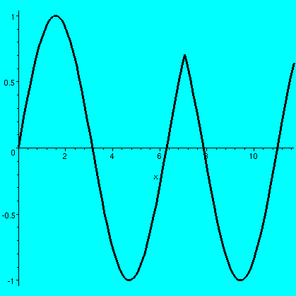
Please note that the pictures here are drawn by Maple in unconstrained mode, filling up the boxes. They are distorted -- the vertical and horizontal axes have different units. The green curve is cosine and the blue curve is sine. I would like to create a piecewise function by taking sine from 0 to its second positive intersection with cosine, and then switching to cosine. This intersection is at 9Pi/4. So the function f(s) is sin(s) for s in [0,9Pi/4] and is cos(s) for s>Pi/4. A graph of it is on the right. First I will express this in terms of Heaviside functions: f(t)=sin(t)+H(t-9Pi/4)(cos(t)-sin(t)). But we want the time-shifted part to be written in terms of t-9Pi/4. Perhaps I could use the Taylor series here, as Mr. Ivanov suggested. But here's another trick. Of course cos(t)=cos((t-9Pi/4)+9Pi/4). Recall (??) that cos(A+B)=cos(A)cos(B)-sin(A)sin(B) so that
cos(t)=cos((t-9Pi/4)+9Pi/4)=cos(t-9Pi/4)cos(9Pi/4)-sin(t-9Pi/4)sin(9Pi/4)=(1/sqrt(2)[cos(t-9Pi/4)-sin(t-9Pi/4)] because both sine and cosine at 9Pi/4 are 1/sqrt(2).
Therefore H(t-9Pi/4)[cos(t)] is H(t-9Pi/4)[(1/sqrt(2)[cos(t-9Pi/4)-sin(t-9Pi/4)], and, since our Laplace transform table contains both sine and cosine, the Laplace transform must be e^-(9Pi/4)s(1/sqrt(2))[s/(s²+1) + 1/(s²+1)]. This is also what Maple got, so I am happy!

The sine part can be dealt with similarly, provided you know a formula for sin(A+B). If you want to do this yourself and check your answer, Maple tells me that the Laplace transform of all of f(s) (once it is simplified) is [1-e^-(9Pi/4)tsqrt(2)]/[s²+1].

I rather daringly attempted problem #42 in section 3.3: an even problem with a large number! Here is the heart of the problem: we want to solve y'-3y=g(t) with the initial condition y(0)=2 and with g(t)=0 for t in [0,4] and g(t)=3 for t>4. Well, g(3) is 3H(t-4) so we need to solve y'-3y=3H(t-4) with y(0)=2. Take the Laplace transform of both sides. We get: sY(s)-y(0)-3Y(s)=e^-4s/s. Here Y(s) is the Laplace transform of the unknown function y(s). Then y(0)=2 so we can "solve" for Y(s). It is Y(s)=e^-4s/[s(s-3)]+2/(s-3). We split up 1/[s(s-3)] so it becomes [-1/s]+[1/(s-3)], all divided by 3. Therefore Y(s)=(1/3)e^-4s([-1/s]+[1/(s-3)])+2/(s-3). Apply Lerch's Theorem, which means we try to do an inverse Laplace transform (look at the Laplace transform tables backwards!). 2/(s-3) comes from 2e^3t and the other part is the inverse Laplace transform of (1/3)(-1+e^3t) time-shifted by 4, and this is H(t-4)(1/3)(-1+e^3(t-4)). Thus y(t) is the sum H(t-4)(1/3)(-1+e^3(t-4))+2e^3t. We might write this is a more traditional form: if t is between 0 and 4, y(t)=2e^3t, and for t>4, y(t)=(1/3)e^3t-12-1/3+2e^3t.

Comments on the solution
Well, for t between 0 and 4, 2e^3t does solve y'-3y=0 with y(0)=2. That's easy to check. And for t>3, y(t)=(1/3)e^3t-12-1/3+2e^3t=[2+(1/3)e^-12]e^3t-1/3, and -1/3 solves y'-3y=3 and the other part is a solution of the homogeneous equation. The Laplace transform is also marvelous in that it selects the two pieces so that together they form a continuous curve. That is, the limit of y(t) from either the left or the right at t=4 is 2e¹², the same number. This is really neat!

The QotD was to compute the inverse Laplace transform of e^-5s(3/s-7/(s-1)+3/[s²+1]. This is a time-shift by 3 of a simple sum of things whose Laplace transforms we know. So it must be 3H(t-5)-7e^t-5H(t-5)+cos(t-5)H(t-5). Alternatively, this function is 0 for t less than 5, and for t>5, it is 3+e^t-5+cos(t-5).

Read the book and do homework problems!

Neat computation #1: sine and cosine
I would like to compute the Laplace transform of sin(t). So the definition tells me that I need to compute ₀^inftye^-stsin(t) dt: o.k. this really isn't too difficult: I would integrate by parts, etc. But I would also like the Laplace transform of cos(t). Here is another way to get them. I remember this formula of euler: e^it=cos(t)+i sin(t). I will compute the Laplace transform of e^it which is easy:
₀^inftye^-ste^itdt=₀^inftye^(-s+i)tdt=[1/(-s+i)]e^-(s-i)t|_t=0^t=infty. The term with t=infty is 0 because e^-st-->0. The other term gives -1/(-s+i). The - sign comes because t=0 is a lower bound.

Now we work with -1/(-s+i): multiply top and bottom by (-s-i). The result is -(-s-i)/(s²+1)=[s/(s²+1)]the real part+i[1/(s²+1)]the imaginary part. But Laplace transform is linear, so L(e^it)=L(cos(t)+i sin(t))=(cos(t))the real part)+iL(sin(t))the imaginary part. Therefore the Laplace transform of cosine is s/(s²+1) and the Laplace transform of sine is 1/(s²+1).

Neat computation #2: lots of bumps
Let's find the Laplace transform of a square wave again. This will be a wave of height 1 from 1 to 2. I will call this SW_[1,2]. What is its Laplace transform? ₀^inftye^-stSW_[1,2]dt=1²e^-stdt=(-1/s)e^-st|_t=1^t=2=(-1/s)(e^-2s-e^-s). There are a number of comments to make here. First, the (nominally) improper integral defining the Laplace transform has become a "proper" integral, and rather an easy one. Second, the Laplace transform actually has only an apparent singularity at s=0. This is because the limit as s-->0 is actually 1 (use L'Hopital, or look at the first terms of the Taylor series of the exponentials).
The Laplace transform of SW_[1,2] is (-1/s)(e^-2s-e^-s).

Graph of SW[1,2]		Graph of its Laplace transform

Let's find the Laplace transform of a square wave again. This will be a wave of height 1 from 3 to 4. I will call this SW_[3,4]. What is its Laplace transform? ₀^inftye^-stSW_[3,4]dt=3⁴e^-stdt=(-1/s)e^-st|_t=3^t=4=(-1/s)(e^-4s-e^-3s).
The Laplace transform of SW_[3,4] is (-1/s)(e^-4s-e^-3s).

I bet that the Laplace transform of SW_[5,6] is (-1/s)(e^-6s-e^-5s).

ETC. By that I mean that we could add up an infinite train of square waves, progressing at integer intervals along the horizontal axis, and have a Laplace transform which is the sum of
(-1/s)(e^-2s-e^-s)+
(-1/s)(e^-4s-e^-3s)+
(-1/s)(e^-6s-e^-5s)+
...

Now the exponentials in each vertical column are geometric series. Here please recall that a+ar+ar²+ar³+...=[a/(1-r)]. The series in the first vertical column is e^-2s+e^-4s+e^-6s+... which is a geometric series whose first term is a=e^-2s and whose ratio is r=e^-2s. Its sum is e^-2s/(1-e^-2s). The series in the second vertical column is e^-s+e^-3s+e^-5s+... and now a=e^-s and r is again e^-2s, so its sum is e^-s/(1-e^-2s). Now package it all together, keeping track of -'s correctly.

The Laplace transform is (-1/s)[(e^-2s-e^-s)/(1-e^-2s)]. O.k., this is not pretty, but it is a real achievement. In all of our calc 1-2-3 courses, and even in 244, we generally looked only at functions defined by nice formulas and gotten tools for them. Here we converted a really horrible function (from that traditional calc point of view), an infinite train of square waves, into a formula. If we can do interesting things with the formula on the Laplace transform side, then we'll be able to really work with the square waves.

Graph of the square wave train

A kind biomedical student pointed out after class that what I created was actually a rather rudimentary model of blood flow driven by a heart beat, so maybe this isn't that silly.

Now let's move on to differential equations, and see how Laplace transform would handle some ODE's we can already solve. First we need to get a formula for the Laplace transform of a derivative.

I want ₀^inftye^-stf'(t) dt to be written in terms of the Laplace transform of f. Since we don't know very much and we have a product of two weird (well, no, let me just write two not obviously related) functions, we could try integration by parts. The suggestion was made that we use u=e^-st and dv=f'(t) dt. Then du=(-s)e^-stdt and v=f(t). The uv term becomes e^-stf(t)_t=0^t=infty. The "infty" goes away because of exponential decay, and the t=0 gives -f(0). The other term is -₀^infty(-s)e^-stf(t). The - sign in front of the integral comes from -integral of v du. The -s is a constant for dt integration, so it comes out. What we have then is L(f')=sL(f)-f(0). The traditional Laplace transform notation seems to be to use capital letters to correspond to small letters of the original function, so the Laplace transform of f is called F. Then written traditionally we have the rule L(f')=sF-f(0). This is Theorem 3.5 in section 3.2 of the text. Another integration by parts gets us L(f'')=s²-sf(0)-f'(0). There are further formulas for higher derivatives.

Solving problems again we can already solve
Everyone who took 244 or a similar course should be able to solve these problems. But here we will try to use the Laplace transform to solve these problems.

Math 244-style problem #1
Solve y''+y=e^t with initial conditions y(0)=0 and y'(0)=0.
Here the homogeneous solutions are sine and cosine, and the particular solution will be some sort of e^t multiple. So the result we get shouldn't look too unexpected. Take the Laplace transform of both sides of the equation. The right-hand side, e^t, has Laplace transform 1/(s-1). I could get this by computation but I would rather look it up (or have Maple etc. compute it). The Laplace transform of the left-hand side is s²Y(s)-sY(0)-Y(0)+Y(s), where Y(s) is the Laplace transform of y(t). The initial conditions immediately imply that the left-had side's transform is just (s²+1)Y(s). Therefore we know that Y(s)=1/[(s²+1)(s-1)]. Now I have been told that it is just "high school algebra" from here. The idea is to decompose the fraction into pieces and recognize each of the pieces as the Laplace transform of a known function. A result quoted in the textbook (Lerch's Theorem is Theorem 3.3 in section 3.1 -- I always liked the name Lerch but only just found out who he was) says that you can reverse the columns of a Laplace transform table, and just "look up" the original function. So I need to decompose 1/[(s²+1)(s-1)] into a sum of terms which I recognize as Laplace transforms, and then use the linearity of Laplace transform and the table of known Laplace transforms. The technique of partial fractions says that 1/[(s²+1)(s-1)] can be written as (As+B)/(s²+1)+C/(s-1). We combine the fractions and look only at the top of each side: 1=(As+B)(s-1)+C(s²+1). When s=1, we get C=1/2. Comparing s² coefficients we get A=-1/2. Comparing the constant terms on both sides we get B=-1/2. So Y(s)=(-1/2)(s/(s²+1)+(-1/2)(1/(s²+1)+(1/2)(1/(s-1)). These pieces are all known Laplace transforms, so we can read off y(t): it is (-1/2)cos(t)+(-1/2)sin(t)+(1/2)e^t. If you are suspicious, you can check this satisfies the ODE and its initial conditions. (I did.)

Math 244-style problem #2
I dared to try an even-numbered problem in the text (but not too high an even number, only 3.2 #2): y'-9y=t with y(0)=5.
The Laplace transform of both sides gives sY(s)-y(0)=1/s². If we use the initial condition we get sY(s)-5=1/s². Solve for Y(s) to get Y(s)=1/[s²(s-9)]+5/(s-9). If I sneak a look into the textbook's table of Laplace transforms, I see that the Laplace transform of e^at is 1/(s-a). So 5/(s-9) is the Laplace transform of 5e^9t. We still must decompose the other term. But (partial fractions again) this is a sum of [A/(s-9)]+[B/s]+[C/s²] and this is As²+Bs(s-9)+C(s-9) (divided by stuff I'll ignore) which should be equal to 1 (divided by the same stuff). If s=9 we get 81A=1 so A=1/81. If s=0, we get -9C=1 so C=-1/9. Comparing s² coefficients gives B=-1/81. Therefore Y(s)=(1/81)[1/(s-9)]+(-1/81)[1/s]+(-1/9)[1/s²]+5/(s-9). Now we use Lerch's Theorem and the table of Laplace transforms to read off the solution:
y(t)=(1`/81)e^9t+(-1/81)(1)+(-1/9)t+5e^9t.
I used Maple to check that this actually worked, because I was exhaust by the end of the computation.

Technology note
Both Maple and Matlab have packages with Laplace and inverse Laplace transforms. I have tried using them, and they sort of work. In Maple you must load the package inttrans and in Matlab you must have the symbolic toolbox.

The QotD was to compute the Laplace transform of the up and down bump SW_[1,2]-SW_[2,3]. I think and hope this was easy.

Please read 3.1 and 3.2 of the text. If you wish to prepare a bit for next week, look at 3.3 and 3.4. Please hand in 3.1: 8,13 and 3.2:9,10 and also compute the Laplace transform of a "tent": a piecewise linear function which is 0 except between A and A+2 (here A is an unspecified positive number). In the interval [A,A+2] the function's graph is a line segment from (A,0) to (A+1,1) and is a line segment from (A+1,1) to (A+2,0). A picture is shown to the right.

How to solve y''+5y'+y=0. Realize this is a linear second order homogeneous ordinary differential equation. Please: students should have had a differential equations course, and should be able to understand the exact meaning of every word of the phrase linear second order homogeneous ordinary differential equation. Ordinary differential equation will be abbreviated "ODE".

In this "linear" is the most important word:

• If y₁ and y₂ are solutions, then y₁+y₂ is a solution.
• If a is a constant (either real or complex, depending on our mood), and y is a solution, then a y is also a solution.

• Numerical methods to approximate solutions
• Qualitative methods (such as phase plane analysis) to learn about limiting behavior or periodicity, etc.

The A and B can be used to specify a unique solution. The simplest example is the initial value problem: y(0) and y'(0) are specified. Then y(0)=A+B and y'(0)=-3A-2B (differentiate and set x=0). any initial conditions can be matched by finding suitable A and B. You should see that this is a consequence of a certain 2-by-2 matrix being invertible. The matrix is

 1  1 
-3 -2

  1   1 
-3e-3  -2e-2

I asked how to solve y''+5y'+y=5e^x, an inhomogeneous equation. We again guess a solution (no, not x³³). We try e^x and "feed it into" y''+5y+6y and get 12e^x and therefore a particular solution will be (5/12)e^x: again we took advantage of linearity. General solutions are gotten by adding the particular solution to solutions of the homogeneous equation.

So we will try to get methods to solve certain linear ODE's. The functions we are interested in are exponentials and sine and cosine and polynomials. But sine and cosine are exponentials also, since e^ix=cos(x)+i sin(x). As for x, it is the limit of (e^rx-1)/r as r-->0 so x is almost an exponential (you can check this assertion with l'Hopital's rule, as we did).

So we need sums of exponentials, indeed, linear combinations of exponentials. Well, linear combinations with many terms are almost integrals, so we should look at weighted sums of integrals of exponentials.

The Laplace transform
We define this by Lf(s)=₀^inftyf(t)e^-stdt. Of course L is supposed to be a script L. This will eventually allow us to solve and analyze certain differential equations better.

We reviewed a bit about improper integrals. I remarked that it is hard to tell by "looking" that as x-->infty, the area "under" 1/x does not have a limit (since ln(R)-->infty as R-->infty) but that the area "under" 1/x² does have a limit (since -1/x-->0 as R-->infty).Things must be carefully computed. Generally functions that decay exponentially will have improper integrals with finite values. I was interested most in the asymptotic behavior of functions in order to analyze {con|di}vergence of improper integrals.

We found that the Laplace transform of the function 1 was 1/s: t is the "time" variable and is used in the integrand. I just directly computed the integral.

We found that the Laplace transform of the function t was 1/s². Here I needed to integrate by parts. The choice of sign in the definition of Laplace transform allows some amazing coincidences to occur (they are not coincidences -- these have been planned to make computation work more easily).

Since exponential decay will always "overpower" polynomial growth (of any degree) any polynomial will have a Laplace transform. Also so will sine and cosine and lots of other things. Although this is nice, what is more interesting is that the Laplace transform will allow us to compute with rough: functions very nicely, functions that commonly arise in real world problems. So I computed that Laplace transform of a square wave: a function given by f(x)=0 for x<3 and for x>7 and f(x)=5 for x in [3,7]. This was easy!

The Laplace transform is linear:

• L(y₁+y₂)=L(y₁)+L(y₂)
• L(ay)=aL(y)

The Question of the Day (QotD) was: tell me the Laplace transform of 3+2t.
Answer I expected that students would use linearity and would use the previously computed Laplace transforms to give the answer (3/s)+(2/s²).

I will do more example of Laplace transforms next time and show how they can be used to solve some ODE's.

Please start reading chapter 3, and begin doing the textbook problems. Hand in the entrance exam on Thursday.
To succeed in this course you will need techniques from calc 2 (such as integration by parts, partial fractions, power series, and improper integrals) and background in basic linear algebra. I'd like some confirmation that you can do what you should be able to, and maybe this confirmation (or other information!) will also help you.