A sort of diary for Math 421:02, spring 2004
Part 4: Fourier series and some classical PDE's

Date	Topics discussed
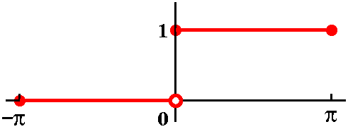
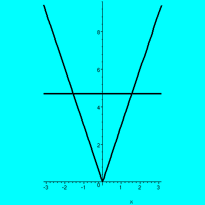
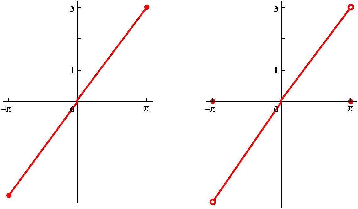
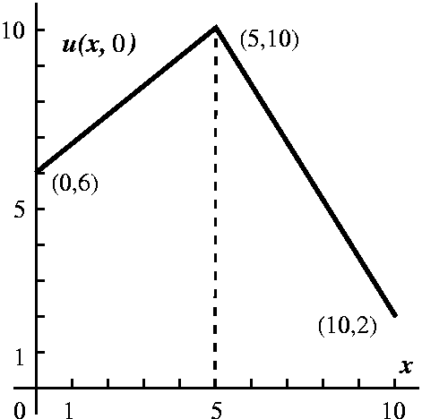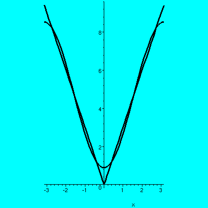
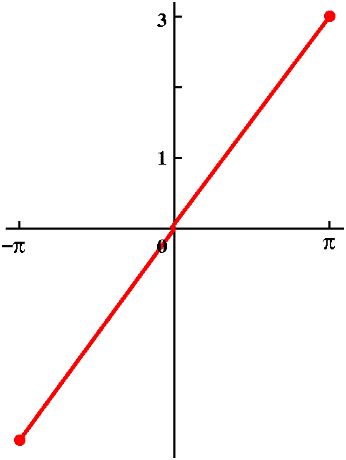
Thursday, April 29	I will begin by asking part 1 of the QotD. The indicated heat distribution is given initially, with boundary conditions u(0,t)=6 and u(10,t)=2. Sketch the limit of u(x,t) as t-->infinity. As we discussed this, I tried to indicate how heat would flow "intuitively". But of course this intuition would be guided by our past thought experiements and computations. Notice that the function -(4/10)t+6 is a steady state heat flow: that is, it has the desired boundary conditions and is only a function of t. Therefore the difference between this function and the u(x,t) in the QotD is a steady state heat flow for the 0 boundary conditions, which must be 0. I also remarked that this initial temperature distribution could not be the result of the time evolution of an earlier temperature distribution. The principle reason for that is because u(x,0) is not differentiable at x=1/2. Temperature distributions which have evolved using the heat equation must be smooth. Then I discussed temperature distributions in a rod with insulated ends (as well as insulated sides). It took some convincing but the appropriate boundary conditions are ux(0,t)=0 and ux(L,t)=0: u doesn't change in the spatial directions across the ends of the bar. I then asked the second part of the QotD: if the ends of the bar are also insulated, what is the limiting heat distribution? Here we want heat not to pile up (I tried to indicate that heat really dislikes being at a local max or min): we want it to distribute itself as well as possible ("entropy", disorganization, should be increasing at all times). Therefore the limiting steady state heat distribution in this case has temperature constant, equal to the average of the initial temperature. In this case, the limiting (average) temperature is 7, and the limiting temperature distribution is the constant 7. I wanted to justify this limiting fact, and to analyze the general boundary/initial value problem for the heat equation: ut= uxx; ux(0,t)=0 and ux(L,t)=0; u(x,0)=f(x) given. So for the fourth time (I think) we analyzed this problem with separation of variables. Assume u(x,t)=X(x)T(t). Then, as before, T'(t)X(x)=X''(x)T(t), so that T'(t)/T(t)=X''(x)/X(x). Again this must be constant, as before. We call it, as before, -. Start with X(x): we know X''(x)/X(x)=-. Again, X''(x)+X(x)=0. The boundary conditions for this equation are from ux(0,t)=0 and ux(L,t)=0. Therefore X'(0)=0 and X'(L)=0. If <0, solutions are linear combinations of cosh(sqrt()x) and sinh(sqrt(x). X'(0)=0 shows that there's nothing coming from the cosh part, and X'(L)=0 shows that the sinh part must vanish, also. Therefore must be positive. Solutions are X(x)=C1sin(sqrt()x)+C2cos(sqrt()x). X'(0)=0 means that C1=0 (the derivative of sine is cosine). And, finally, X'(L)=0 means sin(sqrt()L)=0. Therefore sqrt()L is an integer (usually written, n) times Pi, and =[n2Pi2]/L. What about T(t)? Since T'(t)/T(t)=- =-[n2Pi2]/L, we know that T(t) must must scalar multiples of e-([n2Pi2]/L)t. Notice that if n>0, this -->0 very rapidly, and therefore the only term which persists is the n=0 term. You can check in the book (pp.921-2) to see that the general solution for the time evolution of a heat equation in an insulated bar with insulated ends is u(x,t)=(c0/2+SUMn=1infinitycncos([nPi x]/L)e-([n2Pi2]/L)t where cn=(2/L)0Lf(x)cos([nPi x]/L) dx for n>=0. c0/2 is the average value of f(x) over the interval [0,L], which agrees with the intuition we may have developed giving this constant function as the steady state solution for this problem as t-->infinity. Steady state heat flows in one dimension are solutions of ut=kuxx which are functions of x alone. That is, uxx=0. These functions are just Ax+B where A and B are constants. So these steady state heat flows whose graphs are straight lines have no bumps and no bending. These are the only functions with those qualities. In two dimensions and more, things get more complicated. There steady state heat flows must satisfy uxx+uyy=0. Such functions are called harmonic functions, there are infinitely many linearly independent harmonic functions, and their behavior can be complicated. The room was had numerous gnats in this last class, which plagued bothstudents and instructor. The class ended slightly early. Study for the final exam!
Tuesday, April 27	Derivation of the Heat Equation I tried to "derive" the one-dimensional heat equation, also known as the diffusion equation. You should realize that the heat equation is also used to model a very wide variety of phenomena, such as drugs in the bloodstream diffusing in the body or gossip (!) or spread of disease in epidemics or ... The text discusses the temperature of a thin homogeneous straight rod, whose long side is insulated (no heat flow through that allowed) but heat can escape (or enter) through the ends. I mostly followed the discussion in this web page. Another derivation is given on this page. and yet another is here. If you are someone who learns more easily with pictures, as I do, you may find the various animations of solutions of the initial value problem for the heat equation on this web page useful. Two questions which appear on a web page linked to that reference are interesting to keep in mind: Describe in words the time evolution of a one-dimensional heat flow for which the ends of the bar are both kept at zero degrees. How does your answer depend on the initial temperature distribution? Describe in words the time evolution of a one-dimensional heat flow for which the ends of the bar are kept at different temperatures. How does your answer depend on the initial temperature distribution? Separating ... I separated variables for the initial value problem u(x,0)=f(x) with boundary conditions u(0,t)=0 and u(Pi,t)=0. (The text does this with a more general L instead of Pi.) I assumed a solution to ut=uxx looked like u(x,t)=X(x)T(t), as in the text. The development is very similar to what was done for the wave equation on Tuesday, April 20. I got X''(x)/X(x)=T'(t)/T(t). Therefore each side must be constant. Look at the x side first. The boundary conditions imply that we need to solve the ODE problem X''(x)=(constant)X(x) with X(0)=0 and X(Pi)=0. Therefore to get a non-trivial solution, we must have constant=-(nPi)2 for some positive integer n, and then X(x)=sin(nx). Now here is where we differ from the wave equation: we need to solve T'(t)=-n2T(t). Solutions of this are multiplies of T(t)=e-n2t. Even for small n's this exponential function rapidly decreases from 1 to nearly 0. A general solution would be u(x,t)=SUMn=1infinitycnsin(nx)e-n2t where for the initial value problem u(x,0)=f(x) the cn's would be the coefficients of the Fourier sine series of f(x). 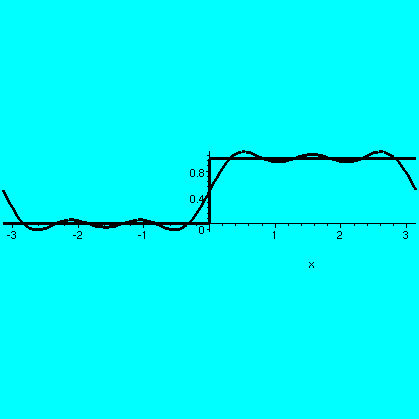What should be expected about heat flow if the ends are kept at temperature 0? We discussed this, and then I gave out this which showed a good approximation to a solution. The heat does flow out, and the heat profile gets smoother. Notice this initial condition is one which I analyzed for the wave equation, and the solutions there were very different. Also notice that the original square profile can't be the result of a heat diffusion (otherwise it would be smooth!) so we can't run the heat equation backwards. The wave equation is time-reversible. Comparing qualitative aspects of solutions of the wave and heat equations Wave equation Heat equation Conservation of energy: in what we studied, the sum of potential and kinetic energy is constant (other models allow friction, etc.) Corners and shocks allowed to persist Finite propagation speed: model has a top speed (speed of sound or light or ...) Time can be reversed: waves just reverse direction, etc. Diffusion: heat oozes away Model is smoothing: even if initial temperature distribution is kinky, for later time, the temperature is smooth Propagation speed turns out to be infinite, but far-off effects for small time are exponentially small. Time can't generally be reversed: you can't make heat flow backwards. I asked what would happen if instead of the boundary condition u(0,t)=0 and u(Pi,t)=0 we substituted u(0,t)=0 and u(Pi,t)=5. First I asked people to think about the physical situation. The general reply is that the temperature distribution would eventually tend to a steady state where one end (at 0) was 0 and the other end, at Pi, was 5. So what I did was write uss(x,t)=(5/Pi)x (this is a guess, but based on the physical suggestion!). It turns out that this uSS ("ss" for steady-state) does solve the heat equation: check that the t derivative is 0 and so is the second x derivative. If we take a solution of the boundary value with u(0,t)=0 and u(Pi,t)=5 (call this solution unew) then unew(x,t)-uss(x,t) does solve the heat equation (since the heat equation is linear) and this solution satisfies the old boundary conditions, u(0,t)=0 and u(Pi,t)=0.But we know because of the )e-n2t factors that this solution must -->0 as t-->infinity. So the difference between unew(x,t) and uss(x,t) must -->0 as t-->infinity. Therefore in fact the steady state is the limit for a solution of this boundary value problem. I should have asked a QotD. It could have been this: suppose one end of a thin homogeneous bar is kept at temperature 7 and the other is kept at temperature -2. Suppose some initial temperature distribution is given (something really complicated). Graph the resulting solution of the heat equation for t=10,000. Think about this: when should I have office hours and possible review sessions for the final? I'll try to do some problems from section 17.2 at the next (last) class.
Thursday, April 22	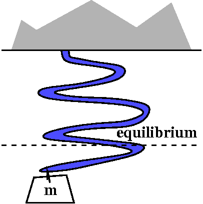The spring, a one-dimensional system Everybody knows the vibrating spring, one of the simplest idealized mechanical systems. Here the dynamics are shaped by Hooke's law, that displacement from equilibrium results in a force of magnitude directly proportional to the absolute value of the displacement and directed opposite to the displacement. This together with Mr. Newton's F=mA gives us D''(t)=-(k/m)D(t) where D(t) is the displacement from equilibrium. The minus sign comes from the word "opposite". Solutions are sines and cosines, yielding the model's solution as vibrating up and down. (A typical vibrating string is the ammonia molecule, NH3.) Looking at energy This model conserves energy, where energy is here the sum of kinetic energy and potential energy. I won't worry about constants, since I can almost never get them right. The kinetic energy is (1/2)m(velocity)2. But velocity is D'(t). What about the potential energy? This is essentially the amount of work needed to move the spring from equilibrium to another position. Well, moving the spring against the varying resistant force of kD(t) means we need to integrate it with respect to D. This gets me (1/2)kD(t)2. The total energy in this model is therefore (1/2)m(D'(t))2+(1/2)k(D(t))2. I can try to check that energy is conserved by differentiating this total energy with respect to time. The result (using the chain rule correctly) is (1/2)m2(D'(t)D''(t))+(1/2)k2(D(t)D'(t)). This is D'(t)(mD''(t)+kD(t)). But the differential equation of motion says exactly that mD''(t)+kD(t) is always 0! So energy is conserved. Both D(t) and D'(t) are sines/cosines, and the sum of their squares is constant (sin2+cos2 is a well-known constant). Taking a static picture at a fixed time can be rather deceptive. For example, if the spring is wiggling (no friction: an ideal spring) it always keeps wiggling. If we happened to snap a picture when the spring is at the equilibrium point it is still moving. The kinetic energy is largest at that position, and the potential energy is smallest. When the spring is highest or lowest, the potential energy is large, and the kinetic energy is 0 (the spring isn't moving, in the sense of calculus: D'(t)=0). I hope that energy considerations will help your understanding of the vibrating string as well as the spring. In fact, we could almost understand the vibrating string as a bunch of springs tied together. This isn't totally correct, but if it helps ... In a very simple case (Warning! big file!) you can see the string in equilibrium position momentarily, but it has relatively high velocity (and therefore large kinetic energy) at that time. The D'Alembert solution: the two waves Here the vibrations of the string are written as a sum of left and right moving waves. Again, y(x,t) is supposed to be the height of the string at time t and position x. We write y(x,t)=K(x-ct)+J(x+ct). Mr. Marchitello helped me to understand that the K part is moving to the right and the J part is moving to the left. Let me use the chain rule: yt(x,t)=K'(x-ct)(-c)+J'(x+ct)c ytt(x,t)=K''(x-ct)(-c)2+J''(x+ct)c2 yx(x,t)=K'(x-ct)+J'(x+ct) yxx(x,t)=K''(x-ct)+J''(x+ct) Now we see that ytt(x,t)=c2yxx(x,t), so indeed this satisfies the wave equation. Comparing initial conditions and the wavea We worked hard to solve (via separation of variables and Fourier series) the initial value problem for the wave equation. For this initial value problem, we considered y(x,0)=f(x) and yt(x,0)=g(x) as given. (Again Mr. Marchitello commented that I seemed to be ignoring the boundary conditions, and I agreed that I was. These details, which are not so trivial, are discussed in the text on pp. 871-872.) So how can we go from the K and J description to the f and g description, and back, and does this help? It turns out that it will help a great deal with the understand of the physical model. Since y(x,t)=K(x-ct)+J(x+ct) we know that y(x,0)=K(x)+J(x)=f(x), and then since yt(x,t)=K'(x-ct)(-c)+J'(x+ct)c we know that yt(x,0)=K'(x)(-c)+J'(x)c=g(x). So this is how we could get f and g from K and J. A short intermission The other example we discussed last time had f(x) equal to 4 on [Pi/3,Pi/2] and 0 elsewhere on [0,Pi], while g(x) was 0 everywhere on [0,Pi]. I produced a picture (Warning! big file!) of a Fourier approximation to this string and its motion through time (for a short period of time). What the heck is going on? Well, we know that K(x)+J(x)=f(x) and (c=1) K'(x)-J'(x)=0, so that K'(x)=J'(x). Can you think of what K(x) and J(x) could be? You are allowed to guess. I can guess, especially when helped by that useful moving picture. K(x) and J(x) are both equal to a bump half the size of f(x): they are both equal to 2 on [Pi/3,Pi/2] and both 0 elsewhere. But one travels left and one travels right. We just happened at initial time to take a picture when the bumps reinforced. When the bumps reach the end of the interval, the boundary conditions (the string is pinned down) cause the bumps to be reflected negatively. Several engineering students seemed to think that this was correct physically. To me much of what is happening in this example is unexpected. Back to the general case We'll try now to get K and J from f and g in general. Let's integrate yt(x,0)=K'(x)(-c)+J'(x)c=g(x) from 0 to x. But first think: should we really write 0xK'(x) dx? There are too many x's. The x's inside the integral could easily get confused with the x on the upper limit of integration. So, following a suggestion of Ms. Sirak, I'll use w for the integration variable. Now we compute: 0xK'(w) dw=K(w)|w=0w=x=K(x)-K(0), and 0xJ'(w) dw=J(x)-J(0). So if I do the arithmetic correctly, the equation K'(x)(-c)+J'(x)c=g(x) leads to [K(x)-K(0)](-c)+[J(x)-J(0)]c=0xg(w) dw or (divide by c, and move J(0) and K(0)): -K(x)+J(x)=(1/c)0xg(w) dw+J(0)-K(0). This together with K(x)+J(x)=f(x) allows me to solve for K(x) and J(x) in terms of stuff involving f and g. Here is what you get: K(x)=-[1/(2c)]0xg(w) ds+(1/2)f(x)-(1/2)J(0)+(1/2)K(0) and J(x)=[1/(2c)]0xg(w) ds+(1/2)f(x)-(1/2)K(0)+(1/2)J(0) I remarked in class and I will repeat now that this is one of the derivations in the whole course that I think is very useful to know about. It really does lead to very useful ideas in the "real world". Let's see: the minus sign in front of the integral for K(x) can be lost if we interchange the top and bottom limits: K(x)=[1/(2c)]x0g(w) ds+(1/2)f(x)-(1/2)J(0)+(1/2)K(0) and also I am really interested in y(x,t). But y(x,t) is K(x-ct)+J(x+ct). So in the formulas for K and J, make the substitutions x-->x-ct in K and x-->x+ct in J. Here is the result for y(x,t): [1/(2c)]x-ct0g(w) ds+(1/2)f(x-ct)-(1/2)J(0)+(1/2)K(0)+ [1/(2c)]0x+ctg(w) ds+(1/2)f(x+ct)-(1/2)K(0)+(1/2)J(0) Now look closely, and see things collapse. Indeed (!) the K(0) and J(0) just cancel. And the integrals? Well, the intervals are adjoining, so the integrals can actually be combined into one. Here is the resulting formula: y(x,t)=[1/(2c)]x-ctx+ctg(w) ds+(1/2)f(x-ct)+(1/2)f(x+ct) By the way, it is natural (to me) that g is integrated. g is a velocity, and y(x,t) is a position. So g's information has to be integrated to get the units to agree. 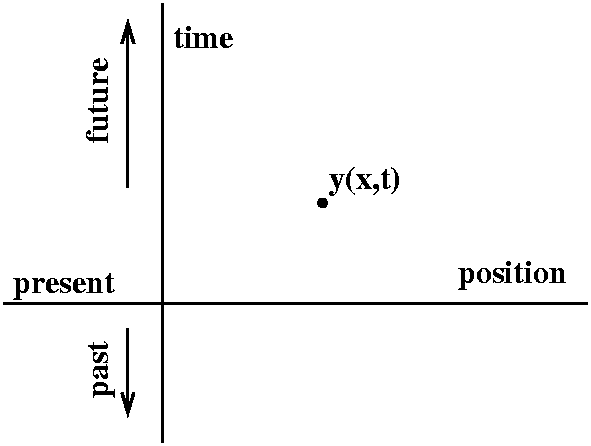Using the formula to understand the physical situation Look to the right. What's displayed is a different way to look at solutions of the wave equation. The function y(x,t) is a function of two variables, one which locates a position on the string, x, and one which indicates time, t. Let's look down on (x,t) space. I would like to know about y(x,t) and what part of the initial data influence y(x,t). Certainly f's values at x+/-ct influence y(x,t) (look at the formula above!) and g's values in the interval [x-ct,x+ct] influence y(x,t). Mr. Tahir bravely came to the board and completed a diagram which looks much like what is draw on the left. The dotted lines have slopes +/-(1/c). (I got this wrong in class!) So the influence of the initial conditions is as shown. 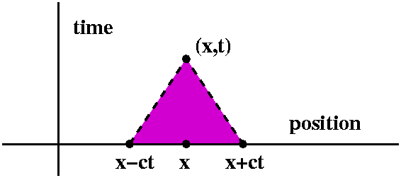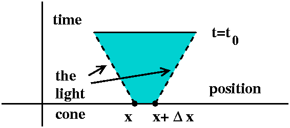Here is yet another way to show what's going on. I could imagine a short interval on the time=0 line, say from x to x+(delta)x (as usual, (delta)x is supposed to be small). I could imagine changing f or g or both on that interval, wiggling these initial conditions. Then what parts of the string could be affected at a later time, t=t0? Well, if you think about it and look at the formula, the only parts could be in the upward part of the trapezoid sketched. The wave equation models phenomena which have a finite propagation speed (here the speed is c). Such phenomena include sound and light. The slanted edges of the trapezoid sketched are usually called the light cone and it represents the spreading the maximum speed that the model allows. This name reflects the physical theory that light travels at the maximum universal speed, and any other "signal" travels more slowly. I remark that Mr. Woodrow courageously drew a picture similar to this on the board. The QotD was ... well ... student evaluations were requested. The local supply of explectives was exhausted. I remarked that the welfare of my family members and pets (alligator, boa constrictor, etc.) depended on these reviews. Ms. Lu kindly agreed to take charge of the evaluations. I wanted to bribe her to fill in the unused ones in a way beneficial to me. This was not done. 16.2: #3 (try n=20 and t=0, t=.5, t=1), #16 a and c, 16.4: #1, #22 (try t=0 and 1 and 2). Please read the text. I remarked that I wanted to spend next week discussing the heat equation, and that I would therefore not cover section 16.7: we don't have enough time. Technically 16.7 covered the wave equation in a rectangle. What's used are several variable Fourier series, but most of the qualitative aspects (about speed of influence, etc.) are much the same as in one variable.
Tuesday, April 20	Copying the book The details of the material in section 16.2 are enormous. To me this material is probably the most daunting (dictionary: discouraging, intimidating) of the whole semester. What I wrote during the beginning of this lecture was essentially copied from the text. Although I have my own opinions about how the material should be organized and presented, my belief is that right now is the wrong time to display the results of these opinions. So here we go: The setup The text starts with a function y(x,t) which is supposed to describe the motion of a string at position x (x between 0 and L) and time t (t non-negative). The string is fastened at the ends, and also has an initial position and velocity. Physical intuition (?!) is supposed to tell you that later positions of the string are determined by these initial conditions and boundary conditions, if y(x,t) obeys the wave equation, ytt=c2yxx. Boundary conditions Here y(0,t)=0 and y(L,t)=0 for all t: the string is fastened down at the ends. Initial conditions y(x,0) is some function f(x) and yt(x,0) is some function g(x). f(x) is supposed to be initial position and g(x) is supposed to be initial velocity. The importance of linearity We will first solve the wave equation with initial data any f(x) and the velocity equal to 0. Then we will solve it with velocity g(x) and initial position equal to 0. The general solution will be the sum of these two solutions. Also important in all this stuff (this is very involved) is that the boundary conditions are homogeneous, so the sum of solutions satisfying the boundary conditions still satisfies the boundary conditions. In what follows I first will ask that y(x,0)=f(x) and yt(x,0)=0 for all x. The boundary conditions lead to eigenvalues via separation of variables The word eigenvalue is also used with differential equations. Please read on. We make the completely wild assumption that the solution y(x,t) can be written as X(x)T(t). This assumption is only being taught to you here because it is useful when considering this equation and a whole bunch of other equations. So learn it! Then (pp.862-863 of the text): XT''=c2TX''. This becomes X''(x)/X(x)=c2T''(t)/T(t). This is sort of a ridiculous equation. The left-hand side is a function of x,and the right-hand side, a function of t. Only constants are such functions. The constant is called -. The reason for the minus sign is to make other computations easier. Since X''(x)/X(x)=-, we get X''(x)+X(x)=0. The boundary condition y(0,t)=0 means that X(0)T(t)=0 for all t. Well, if the T(t) isn't supposed to be 0 always, we must conclude X(0)=0. Similarly the boundary y(L,t)=0 yields X(L)=0. So we are led to the problem: X''(x)+X(x)=0 with X(0)=0 and X(L)=0. What can we say about the boundary value problem for this ordinary differential equation? Well, I know a solution for it. The solution X(x)=0 for all x is a solution. This resembles what happens in linear homogeneous systems. There's always the trivial solution. Are there other solutions? Consider the following. Stupid example Suppose we are looking for a solution to X''(x)+56X(x)=0 and X(0)=0 and X(48)=0. Well, solutions to X''(x)+56X(x)=0 are C1sin(sqrt(56)x)+C2cos(sqrt(56)x). If X(0)=0, then since cos(0)=1 and sin(0)=0, this means C2=0. So the solution is now C1sin(sqrt(56)x). But if X(48)=0, we plug in x=48: C1sin(48sqrt(56))=0. When is sin(x)=0? It is only when x is an integer multiple of Pi. But I don't think that 48sqrt(56) is an integer multiple of Pi. (Check me, darn it: compute [48sqrt(56)]/Pi and see if this is an integer!) This means that if the equation C1sin(48sqrt(56))=0 is true, then C1=0. Therefore (blow horns and pound drums!!!!) the boundary value problem X''(x)+56X(x)=0 and X(0)=0 and X(48)=0 has only the trivial solution. O.k., back to the general case: X''(x)+X(x)=0 and X(0)=0 and X(L)=0. The solutions are C1sin(sqrt()x)+C2cos(sqrt()x). The X(0)=0 condition gives C2=0. What about inserting x=0 in the other piece? C1sin(sqrt()L)=0 has a solution with C1 not equal to 0 exactly when sqrt()L=nPi for an integer n. Then is [n2Pi2]/L2. Selecting as one of these values (with n=1 and n=2 and n=3 and ...) allows the possibility of non-trivial solutions. If is not only of these values then the only solutions are the trivial solutions. These special values of are called the eigenvalues of this boundary value problem. Now let's consider the T(t) function. Well, (1/c2)T''(t)/T(t)=- (where is now identified as above!). So T''(t)+[n2Pi2c2]/[L2]T(t)=0. We haven't used the initial condition yt(x,0)=0 for all x. This leads to T'(0)X(x)=0 for all x. Again, either we have a really silly (and trivial) solution X(x)=0 always or we require that T'(0)=0. So if we know that T''(t)+[n2Pi2c2]/[L2T(t)=0 then T(t)=C1sin([nPi c/L]t)+C2cos([nPi c/L]t). What's T'(t)? It has a sine and a cosine, and requiring that T'(0)=0 menas that the coefficient in front of cosine (in the derivative!) must be 0. Then C1 must be 0. So T(t) is C2cos([nPi c/L]t). We then get the solution y(x,t)=X(x)T(t) is (CONSTANT)sin([nPi/L]x)cos([nPi c/L]t). Here again n is a positive integer. We have done lots of work to get to this place. 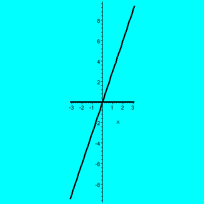Linearity of the wave equation When t=0 in the solution listed above we get (CONSTANT)sin([nPi/L]x). So if you (we?) happen to be lucky, and your c=1 and your L=Pi and your initial position is 36sin(5x) then you can just "guess" a corresponding solution to the wave equation: 36sin(5x)cos(5t). Below to the left is the initial shape of this wave form. Then to the right is an animation of what happens as t goes from 0 to 4. The pictures are linked here. Warning! Large file (~1 meg) to be transmitted. Remember this is for an idealized vibrating string with no friction, etc., so it just keeps going back and forth endlessly (remember Hooke's law and its validity: the ideal spring compared to a spring vibrating in thick honey, etc.) Energy is constant in this system. When the string at max amplitutde, it is not moving: all the energy is potential. When the string overlays to x-axis, its energy is all kinetic. This is indeed just like an idealized vibrating spring. But what happens if we want a more complicated initial wave? Well, we take advantage of linearity. We can add up the simple waves, and we get y(x,t)=SUMn=1infinitycnsin([nPi/L]x)cos(nPi c/L]t) (this is on p.864 of the text). When t=0, this becomes y(x,0)=SUMn=1infinitycnsin([nPi/L]x) since cosine of 0 is 1. Let me do an example. Here I will suppose that c=1 and L=Pi. Then y(x,0)=SUMn=1infinitycnsin(nx). 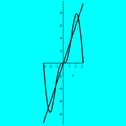Let me ask that the initial shape of the string be like this: 0 if x<Pi/3 or if x>Pi/2, and 4 for x in the interval [Pi/3,Pi/2]. This is a rectangular bump, and please ignore the fact that it is not continuous. I would like to represent this function as a sum of sines. We have the technology: we can extend the function as an odd function and compute the Fourier coefficients. 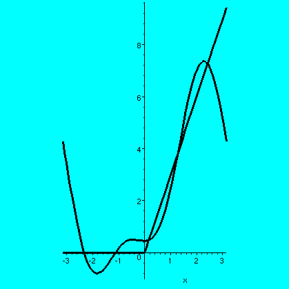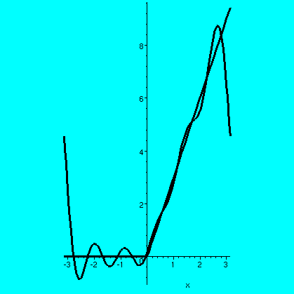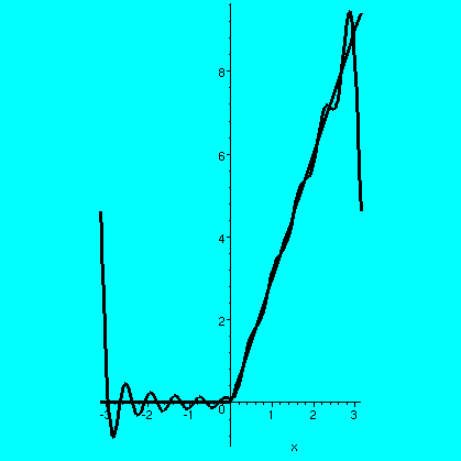Here is the result graphically. The picture on the left shows the original rectangular bump, and compares it with the sum of the first 40 terms of the Fourier sine series (obtained by extending the function in an odd way to [-Pi,Pi]). This static picture shows the usual phenomena, including the Gibbs over- and undershoot. The next picture shows the resulting vibration, if you can follow it, during the interval from t=0 to t=4. Notice that fixing the boundary points at 0 "reflects" the waves in a reversed fashion off the ends. This is quite fascinating to me. The pictures are linked here. Warning! Large file (~1 meg) to be transmitted. The initial value problem (velocity) Here I suppose that y(x,0)=0 for all x, and yt(x,0)=g(x), for x in [0,L]. Almost the same computations are used. Look at p. 868. In this case, the boundary value problem for the t variable makes the cosine term vanish, because y(x,0)=X(x)T(0)=0. So here y(x,t)=SUMn=1infinitycnsin([nPi/L]x)sin(nPi c/L]t) and you find the cn's from the derivative: yt(x,0)=SUMn=1infinitycn[nPi/L]sin([nPi/L]x)=g(x) where the coefficients are from the sine series of g(x). Wow. I don't want to make more pictures because the storage space needed for the animated gifs is enormous. So what can you do ... Not much is easy to do by hand. I would sincerely hope that anytime you need to work with these things, you will have a program like Maple or Matlab or Mathematica at hand. Waves, moving right and left I think it was Mr. Sosa who kindly let me use the string from the hood of his jacket to show a rather different representation of the wave shapes. I wiggled one end, and Mr. Sosa wiggled the other. The result was something like what I show below. Here is an example of a solution to the wave equation which I checked in class: y(x,t)=(x-t)342+(x+t)221 To check this you must remember the Chain Rule carefully. The precise numbers don't matter. It turns out that the dependency on x+t and x-t are the only things that matter. As t grows, the x-t part represents a wave moving to the right and the x+t part represents a wave moving to the left. This is called the D'Alembert representation of the solution, and I will try to understand it more on Thursday and connect it with the work done earlier. Please look at section 16.4 of the text. 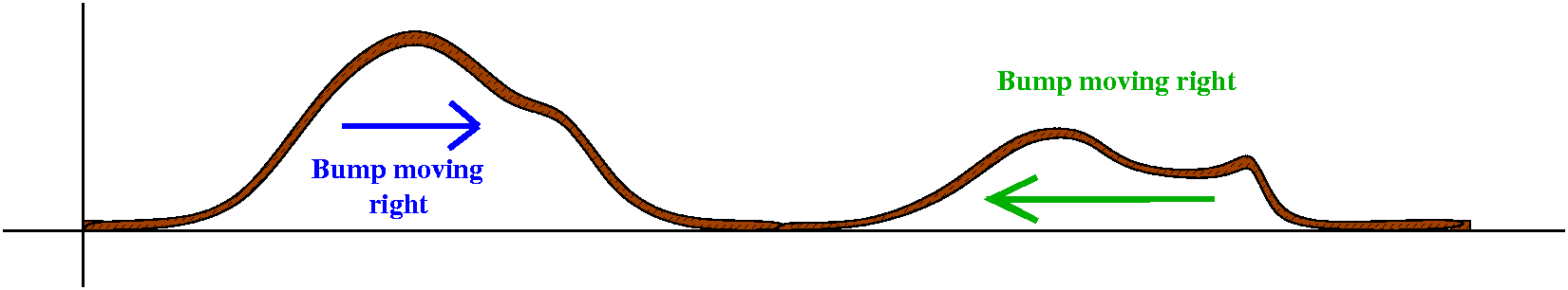The QotD was to look at two bumps, one moving right and one moving left, and draw a picture some time later of what the profile would look like. It was not a wonderful QotD. Please read the text!
Thursday, April 15	Homework: DONE 13.2 #9, was presented on the board (thanks to Mr. Araujo), 13.3 #5, was presented on the board (thanks to Ms. Mudrak), and 13.5 #2, was presented on the board (thanks to Mr. McNair). These problems all had their technical difficulties (especially 13.3, #5, when done "by hand") but are all straightforward applications of formulas in the tex. PDE's In 244 you learned about ordinary differential equations and initial value problems. The basic theory can be stated easily: a nice ODE with the correct initial conditions (order n equation with n initial conditions) has a solution. Of course, "solving" an ODE, in the sense of getting a neat symbolic solution or even approximating the solution well, required tricks and lots of thought. But the theory is there. By contrast, partial differential equations are horrible. The equations we will analyze in the short time remaining in this course (the classical wave and heat equations) have been studied a great deal for two hundred years, but even these PDE's have properties which are difficult to understand, both theoretically and computationally. More general PDE's have very little theory supporting their study. This is a pity, because many "real" phenomena are best modeled by PDE's. The Wave Equation The wave equation is an attempt give a mathematical model of vibrations of a string (space dimension=1) and a thin plate (space dimension=2). Please read the assigned sections in the text in chapter 16. It will be very helpful if you read these sections in advance, since the computational details are intricate! In one dimension, the wave equation described the dynamics of a string imagined drawn over the x-axis, whose height at position x at time t is y(x,t), and gets a condition which is satisfied by y(x,t): ytt=c2yxx. Here the subscripts tt and xx refer to partial derivatives with respect to time (t) and position (x). To me, a really neat part of the subject is discovering why this equation is true, based on simple physical assumptions. Here and here are two derivations of the wave equation I found on the web. Please note that the wave equation describes small vibrations of an idealized homogeneous string. If your string is lumpy (?) or if you want to pull it a large amount, then such a simple description is not valid. The wave equation will model fairly well the motion of a guitar string, say. One nice thing to notice is that ytt=c2yxx is linear: if y1 and y2 are solutions, then the sum y1+y2 is a solution, and so is ky1 for any constant k. So the solutions of the wave equation form a subspace. This is frequently called the principle of superposition (yeah, there are over 86,000 web pages with this phrase!). A random function is not likely to solve the wave equation, which essentially asks that yxx and ytt be constantly proportional: that's quite a stiff requirement. Here are some candidates and how I might check them: y(x,t) yt ytt yx yxx Constantly proportional? x5+t3 3t2 6t 5x4 20x3 No! t3ex 3t2ex 6tex t3ex t3ex No! sin(xt) x cos(xt) -x2sin(xt) t cos(xt) -t2sin(xt) No! cos(x2+5t) -5sin(x2+5t) -25cos(x2+5t) -2x sin(x2+5t) -2sin(x2+5t)-4x2cos(x2+5t) No! sin(3x)cos(5t) -5sin(3x)sin(5t) -25sin(3x)cos(5t) 3cos(3x)sin(5t) -9sin(3x)cos(5t) Yes! c2=9/25 e4tcos(5x) 4e4tcos(5x) e4tcos(5x) -5e4tsin(5x) -25e4tcos(5x) No!   The constant of proportionality, c2, must be positive! log(6x+7y) 7/(6x+7y) -49/(6x+7y)2 6/(6x+7y) -36/(6x+7y)2 Yes! c2=49/36 My reasons for compiling this table are to warm up by computing some partial derivatives in case you have forgotten how, and, more seriously, to show you how rarely the equation is satisfied. 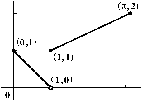Setting up a boundary value problem The physical aspect of the wave equation is important in what we should expect of solutions. It turns out that there are lots of solutions, but which ones will make physical sense? Here maybe it does help to think of a guitar string. Again, I'll follow the text closely (please read the text!). Usually the guitar string is fastened at the ends, so right now we will assume y(0,t)=0 and y(L,t)=0. 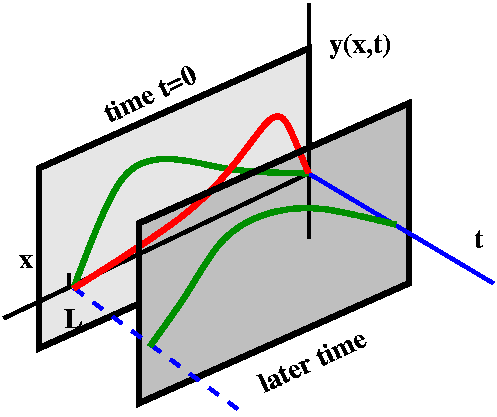But we need to know more information: we need the position of the string at time t=0, y(x,0) for x in [0,L], and, further, we need to know the velocity of the string at time t=0, yt(x,0) for x in [0,L]. To the right is my effort to show you a picture of what is happening. There is an x-axis on which the string is "vibrating". The other horizontal axis is t, time. Time is progressing futurewards (?) as t increases. The height from the (x,t) plane is y(x,t), the string's height at time t and position x. Then y(x,t) actually describes a surface, and each slice with a fixed time, t, is a frozen picture of where the string is at time t. I specify that the string is fixed at height 0 (blue line and dashed line) at x=0 and x=L. But I also specify the initial position when t=0 (that's the green curve) and the initial velocity when t=0 (that's the red curve). The red curve declares that the string is moving up when t=0, and moving up faster when x is small than when x is large. I also tried to show a picture of the string for a little bit later time, and, indeed, wanted to make clear that the part of the string for x small has moved up more than the part for x large. This is a complicated and maybe silly picture. You can look at it, but maybe you should also try creating your own pictures. Your own pictures will likely make more sense to you. The boundary conditions y(0,t) and y(L,t) and the initial conditions y(x,0) and yt(x,0) for x in [0,L] are generally what people expect with the wave equation. Recognizing that these conditions are appropriate comes from the physical situation. Trying to solve the wave equation There are several standard techniques for solving the wave equation. Here is one of them, called separation of variables. Look at ytt=c2yxx and assume that y(x,t)=X(x)T(t): that is, y(x,t) is a product a function of x alone and a function of t alone. Then ytt is X(x)T''(t) (you may need to think about this a bit!) and yxx is X''(x)T(t). If this weird function satisfies the wave equation, then X(x)T''(t)=c2X''(x)T(t) so that T''(t)/T(t)=c2X''(x)/X(x). On the left side of this equation we have a function of t alone, and on the right side of the equation, we have a function of x alone. The only function that is a function of both x alone and t alone is a constant. This constant is usually called - (sorry about the minus sign, but everyone uses it, and you will see why, very soon). Therefore, if X(x)T(t) solves the wave equation, I know that T''(t)/T(t)=- so that T''(t)+T(t)=0 and I know a similar statement for X(x). So now I'll use what I know about ODE's to find eligible T(t) and X(x). Please look at the textbook. I will continue this next time. A proposal for the Final Exam I suggested that instead of having a comprehensive final covering all parts of the course that I do the following: Write an exam, whose length and difficulty will be appropriate (similar to the past two exams) covering the Fourier series part of the course. Everyone would take this, and I would grade it, and count it as one of three similar exams in the course. Optionally offer a few problems on linear algebra and a few problems on Laplace transforms for students who wish to improve their grades in the exams. After some discussion and e-mail with students, I would like to specify the possible improvement so that no one can get more than 100. Here is one strategy, which is historically and physically interesting: if a student got GLT on the Laplace transform grade, and then got PLT on the optional few Laplace transform problems then (GLT is in the interval [0,100) and PLT, in the interval [0,{20 or 25 or 30}], I would replace (for term grade purposes) GLT by (GLT+PLT)/(1+GLT·PLT/104). Some of you may recognize this as Lorentz addition of grades! So the Lorentz sum of 55 and 15 is 64.67 (I'll use approximations here). Using this formula, students could never score more than 100. Comment and information Here is a quote from a web page entitled How Do You Add Velocities in Special Relativity?: w = (u + v)/(1 + uv/c2) If u and v are both small compared to the speed of light c, then the answer is approximately the same as the non-relativistic theory. In the limit where u is equal to c (because C is a massless particle moving to the left at the speed of light), the sum gives c. This confirms that anything going at the speed of light does so in all reference frames. I think this penalizes students who got a fairly good grade already too much, though. For example, the Lorentz sum of 75 and 15 is only 80.90. So maybe I should find something better. There was no QotD! But I did ask people to: Begin reading the sections of chapter 16. Please hand in 13.5, #3 and #4, and 16.1, #4.
Tuesday, April 13	I had prepared a sequence of handouts, which are reproduced here as gifs. I basically wanted to discuss a sequence of examples to illustrate The definition and computation of Fourier coefficients. The behavior of the partial sums of Fourier series. The (theoretical?) limiting behavior of the partial sums of Fourier series: what is the sum of the whole Fourier series? The qualitative behavior of the Fourier series. The Parseval equality. Odd and even extensions of functions and the Fourier sine and cosine series which result. This is a lot to think about but we can only complete this by beginning, so let's begin. I remarked that Taylor series are good for "local" computations near a fixed point, in some "tiny" interval around the point. Fourier series are a wonderful thing to use on a whole interval. I recalled some general facts: the definitions of Fourier coefficients and Fourier series and how the partial sums and the whole sum of the Fourier series behaves compared to f(x). I also supplied a (very short) table of integrals we would need today: Function Antiderivative cos(Kx) (1/K)sin(Kx)+C sin(Kx) -(1/K)cos(Kx)+C x cos(Kx) (1/K)x sin(Kx)+(1/K2)cos(Kx)+C x sin(Kx) -(1/K)x cos(Kx)+(1/K2)sin(Kx)+C A first example (an old QotD) My first example analyzed the QotD from the previous regular class meeting. So f(x) is 0 for x<0 and is 1 for x>=0. In everything I am doing today, I will only care about the interval [-Pi,Pi]. If you run across a situation where you "care" about the interval [-5,11], say, probably you should first take x and change it into y=(2Pi/16)x-(3Pi/8). Then as x runs from -5 to 11, y would go from -Pi to Pi. Anyway, I used the following Maple commands to create the pictures I will show and also the resulting computations. Maple commands Here is how to write f(x), a piecewise defined function: f:=x->piecewise(x>0,1,0); This command creates a function q(n) which produces the cosine Fourier coefficients: q:=n->(1/Pi)*int(f(x)*cos(n*x),x=-Pi..Pi); and here is r(n) which produces the sine Fourier coefficients: r:=n->(1/Pi)*int(f(x)*sin(n*x),x=-Pi..Pi); Here I have a function Q(k) which creates a pair of functions. The first element of the pair is f(x), and the second element of the pair is the partial sum of the Fourier series up to the terms sin(kx) and cos(kx): Q:=k->{f(x),(1/2)*q(0)+sum(q(n)*cos(n*x)+r(n)*sin(n*x),n=1..k)}; And then this command produces a graph of the previous pair. QQ:=n->plot(Q(n),x=-Pi..Pi,scaling=constrained); I try to write short and simple Maple commands rather than write big programs. I can't understand big programs easily. So all four of the pictures below were produced by the one command line (one: only one!) QQ(0);QQ(2);QQ(5);QQ(10); f(x) and the partial sums of the Fourier series for f(x) up to n=0 n=2 n=5 n=10 The hard part of this is figuring out what we can learn from such pictures. I mention that these pictures and the others I'll show below would be really irritating to obtain (at least for me!) without technological help. Observation 1 Please realize that the partial sums (which are linear combinations of sin(mx) and cos(nx)) will always have the same values at -Pi and Pi since sin(mx) and cos(nx) are the same at -Pi and Pi. So these functions really "wrap around" on the [-Pi,Pi] interval. Look at the pictures! Observation 2 The first picture tells me that (1/2)a0, that horizontal line, which here has height 1/2, is the mean square best constant approximating our f(x). That is, if I sort of take values at random, then the horizontal line will have the least error, on average, from the function's value. I hope you can see this here, since the function involved is quite simple. 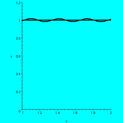Observation 3 Go away from the jumps in the function. That is, imagine you restrict your attention to x between -Pi and 0 or x between 0 and Pi. What's happening there? Here's a picture of a piece of the graph of f(x) and the partial sum, with n=20, in the interval for x between 1 and 2, away from the discontinuities. You should notice that the error between the function and the partial sum is very very small. In addition, the partial sum, in this restricted interval, really does not wiggle very much. That is, its derivative is quite close to 0. The derivative of f(x) is 0 oin this interval, of course, since it is a horizontal line segment. 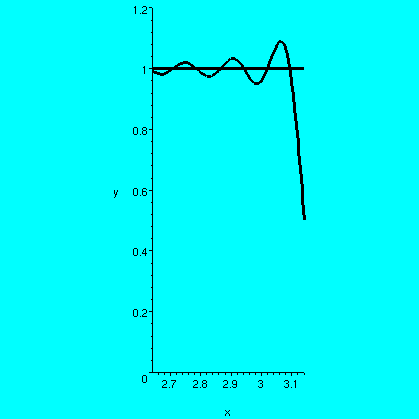Observation 4 Here by contrast is a picture of what happens to the 40th partial sum (I'm very glad I'm not doing these by hand!) and f(x) on the interval [Pi-.5,Pi]. Of course (observation 0) the partial sum hops "down" towards 1/2 at x=Pi. But it is sort of interesting (as Mr. Dupersoy noticed!) that there is sort of an overshoot. The overshoot is very very near the jump. I will come back and discuss this a bit later. The overshoot (which has an accompanying "undershoot" for this f(x) at -Pi) is called Gibbs phenomenon, and is rather subtle. The sum of the whole Fourier series Theory tells me what the sum of the whole Fourier series should be. This function f(x) is "piecewise smooth". Theory then says that the sum of the whole Fourier series is f(x) if x is a point where f(x) is continuous. 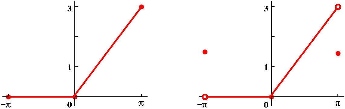If the left- and right-hand limits of f(x) exist at a point and if these limits are different, then the Fourier series attempts to compromise (!) by converging to the average of the two values: graphically, a point halfway in between the limiting values of f(x). In our specific case, there are three (well, two, if you consider -Pi and Pi to be the "same" which they are for sine and cosine) points of discontinuity: -Pi, 0, and Pi. At each of those, the whole Fourier series of f(x) converges to the values shown. Maple code for Parseval This command s:=k->(1/2)*q(0)^2+sum(q(n)^2+r(n)^2,n=1..k); adds up the Fourier coefficients (properly squared) and is a partial sum of the infinite series appearing on one side of the Parseval formula. pars:=k->[s(k),evalf(s(k)),(1/Pi)*int(f(x)^2,x=-Pi..Pi),evalf((1/Pi)*int(f(x)^2,x=-Pi..Pi))]; asks Maple to produce four quantities: the first one is the partial sum of the Parseval series symbolically evaluated (if possible), the second is a numerical approximation to that sum, the third is the integral symbolically evaluated (if possible), and the fourth is a numerical approximation to that integral. The command pars(10) gives the response 469876 [1/2 + ---------, 0.9798023932, 1, 1.] 2 99225 Pi and pars(20) gives the response 204698374253288 [1/2 + ------------------, 0.9898762955, 1, 1.] 2 42337793743245 Pi Observation 5 (and something sneaky!) Well, at least .989... is closer to 1 than .979..., so maybe the partial sums of the Parseval series are equal to one. Well, to tell you the truth, very few people in the real world use the Parseval series to compute the integral of f(x)2 on the interval [-Pi,Pi]. Instead, things like the following are done. What's an? It is (1/Pi)-PiPif(x) cos(nx) dx, which is (for our specific f(x)!) (1/Pi)0Picos(nx) dx=(1/(nPi))sin(nx)|0Pi. But sine at integer multiples of Pi is 0, so an is 0. Errrr .... except for n=0, when that formula is not valid. We know that a0=1 (compute the integral of f(x)2, which is 0 on the left and 1 on the right!). What's bn? It is (1/Pi)-PiPif(x) sin(nx) dx, which is (for our specific f(x)!) (1/Pi)0Pisin(nx) dx=-(1/(nPi))cos(nx)|0Pi. Now cos(n0) is cos(0) which is 1. What about cos(nPi)? It is either +1 or -1, depending on the parity (even/odd) of n. In fact, it is (-1)n. Therefore we have a formula: bn=(1/(nPi))((-1)n+1). (I screwed up this calculation in class!) What the heck does the Fourier series of f(x) look like? If you try the first few terms (all of the cosine terms are 0 except for the constant term!) you will get: (1/2)+(2/Pi)sin(x)+(2/(3Pi))sin(3*x)+(2/(5Pi))sin(5*x)+(2/(7Pi))sin(7*x)+(2/(9Pi))sin(9*x)+... Actually, what I did was just type the command sum(r(n)*sin(n*x),n=1..10); into Maple, copy the result and add on (1/2) in front. This allowed me to check all of my computations. Then the infinite series in Parseval becomes (1/2)+(4/Pi2)SUMn=0infinity1/(2n+1)2 where I factored out the 4/Pi2 from each term (uhhhh: 4/Pi2 is the square of 2/Pi). So we actually have (now put in (1/Pi)-PiPif(x)2 dx, which in our case is just 1): 1=(1/2)+(4/Pi2)(the big SUM). We can solve for the sum. And thus (non-obvious fact coming!) The sum of 1/(all the odd squares) is Pi2/8. Maple evidence for this silly assertion I tried the following: evalf(sum(1/(2*n+1)^2,n=0..100)); 1.231225323 evalf(Pi^2/8); 1.233700550 which compares the sum of the first 100 terms with Pi2/8. And then, heck, what's time to a computer?, I tried the first 1000 terms: evalf(sum(1/(2*n+1)^2,n=0..1000)); 1.233450800 But the convincing command is this: sum(1/(2*n+1)^2,n=0..infinity); 2 Pi --- 8 because Maple can recognize certain infinite series and "remember" their values! The second example Here f(x) is the function 3x for x>0, and f(x)=0 for x<0. Here are some pictures: f(x) and the partial sums of the Fourier series for f(x) up to n=0 n=2 n=5 n=10 I hope you can see some of the same qualitative features in these pictures as in the previous collection. So you should see in the first picture the best constant that approximates this f(x). In the succeeding pictures, you should see better and better approximations, away from the points of discontinuity (Pi, -Pi, which the trig functions regard as the "same"). 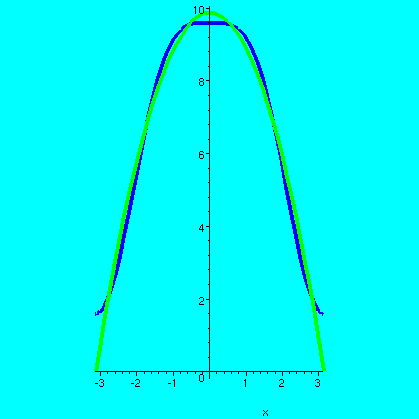Even the derivatives of the partial sums (for x not 0 or +/-Pi) are approaching the derivatives of f(x). There's also a Gibbs phenomenon, the bumps at +/-Pi. Here is:          A graph of f(x)                        A graph of the sum of                        the Fourier series for f(x) Some Fourier coefficients for this f(x) I tried to compute a11. This is (1/Pi)-PiPif(x) cos(11x) dx=(1/Pi)0Pi3x cos(11x) dx (because f(x) is 0 for x<0). I can antidifferentiate this (especially with the table above!). So it is (3/(11))x sin(11x)+(3/(11)2)cos(11x)|0Pi. I know that sin(11Pi) and sin(0) are 0. Also cos(0)=1 and cos(11Pi)=-1, so after computing, -6/(121Pi). How about b10? This is (1/Pi)-PiPif(x) sin(10x) dx=(1/Pi)0Pi3x sin(10x) dx and this is -(3/10)x cos(10x)+(3/(10)2)sin(10x))|0Pi, and, evaluating carefully, this will be -3/(10). Hey: I just wanted to show you that some of each kind of Fourier coefficient is not 0. Cheap cosines? We have seen that 3x, for x between 0 and Pi, is some crazy infinite linear combination of sines and cosines. What if evaluating cosines was very very cheap and easy, and evaluating sines was really expensive. I will show you a clever way to get 3x, for x between 0 and Pi, as a sum only of cosines. The even extension Fold over 3x on [0,Pi]. That is, define f(x) to be 3x for x>0 and f(x) is -3x for x<0. Then the resulting new f(x) is even, so that multiplying it by sin(mx), an odd function, and integrating the product from -Pi to Pi must result in 0. The Fourier series of this new function has only cosine terms. 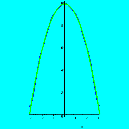f(x) and the partial sums of the Fourier series for f(x) up to n=0 n=2 n=5 n=10 We're using only cosines, and the two graphs look really close for n=10. The function and the sum of the whole Fourier series are identical in this case (the function is continuous in [-Pi,Pi] and its values at +/-Pi agree). The odd extension Change the game, so that now computing sines is cheap, and cosines are impossibly expensive. So we take 3x on [0,Pi] and extend it to an f(x) on [-Pi,Pi] with f(-x)=f(x). This has a simple algebraic definition (no longer piecewise): f(x)=3x for x in [-Pi,Pi]. Nows the integrals defining the cosine coefficients are 0 (cosine is even, this f(x) odd, so the product is odd). Here are the pictures which result: f(x) and the partial sums of the Fourier series for f(x) up to n=0 n=2 n=5 n=10 Again, I hope you see some neat qualitative aspects.          A graph of f(x)                        A graph of the sum of                        the Fourier series for f(x) These graphs differ at the endpoints. What are these darn things? I asked Maple to compute the beginnings of each Fourier series and I display the results. Please note (it is almost unbelievable!) that each of these series has the same sum, 3x, for x in the interval [0,Pi). Picture Beginning of the Fourier series Original f(x) 3 Pi 5 cos(x) 3 2 cos(3x) ---- - -------- + 3 sin(x) - - sin(2x) - -------- + sin(3x) 4 Pi 2 3 Pi Even extension from [0,Pi] 3Pi 12 cos(x) 4 cos(3x) 12 cos(5x) --- - --------- - --------- - ---------- 2 Pi 3 Pi 25 Pi Odd extension from [0,Pi] 3 6 6 sin(x) - 3 sin(2x) + 2 sin(3x) - - sin(4 x) + - sin(5 x) 2 5 The Maple command I used here was (1/2)*q(0)+sum(q(n)*cos(n*x)+r(n)*sin(n*x),n=1..5); separately for each function. The Gibbs phenomenon: (maybe) a simpler version Here is a simple model situation to help you understand the Gibbs phenomenon. I don't know any particular "real" application that needs to pay attention to this overshoot idea, but lots of people (about 44,500 web pages mention it, according to Google!) are curious about it. In 1863, J. Willard Gibbs received the first U.S. doctorate in engineering. He saw that at a jump discontinuity, there is always an overshoot of about 9% in the Fourier series. The limit of the overshoot's behavior vanishes! This is a bit difficult to understand at first. 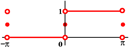Here are some pictures of a similar situation which may help you. 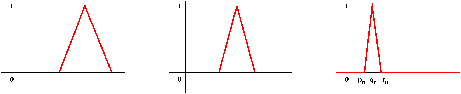This is a picture of a moving bump. The bump is always non-negative, and is always 1 unit high. It gets narrower and narrower as n increases, and moves toward, but never actually reaches, 0. The point pn is at 1/n, and qn is at 2/n, and rn is at 3/n. The graph is made of four line segments. Notice that if you "stand" at 0, you never feel the bump. Of course, you also never will feel the bump if you are at any negative x. But, and this is most subtle, if x is positive, then for n large enough, the bump eventually passes you, goes toward 0, and your value goes to 0 and stays at 0. So the limit function of this sequence of moving bumps is 0 at every point, but each bump has height 1! This is similar to the bumps found by Gibbs. The partial sums display a sort of moving bump effect, but the limit function (the sum of the whole series) doesn't show any additional bump. The QotD was: here is a function given graphically on the interval [0,Pi]. The answer(s) will be a series of four graphs. First, graph the odd extension of this function to [-Pi,Pi]. Then draw the graph of the sum of the whole Fourier series of the odd extension on the interval [-Pi,Pi]. For the third graph, draw the even extension of this function to [-Pi,Pi]. Then draw the graph of the sum of the whole Fourier series of the even extension on the interval [-Pi,Pi].
Thursday, April 8	We had fun with the linear algebra exam, and only about a quarter of the students stayed past 10 PM.
Tuesday, April 6	Real-life linear algebra [ADVT] One step in the algorithm used by Google to develop PageRank (a way of deciding which pages are more reputable or useful) is finding the largest eigenvalue of a matrix which is about three billion by three billion in size. This is a ludicrous but real application of linear algebra. I have no idea how to effectively compute such a thing. End [ADVT] I tried again to discuss closest approximation, but I am willing to concede that this approach to Fourier series does not seem to resonate with students. Perhaps it is my fault. I may not have prepared the territory enough in linear algebra. We will start with a function f(x) defined on the interval [-Pi,Pi]. In Fourier series, we try to write f(x) as a sum of sines and cosines. That is, I want to write f(x) as a linear combination of cos(nx) and sin(nx), where n and m are non-negative integers. As to cos(nx), the term corresponding to n=0 is somewhat special: cos(0x) is the constant 1. We can discard sin(0x) since sin(0x) is 0. There are various constants that come up which occur so that orthogonal functions are orthonormal. Here's a general approach which is useful in many integrals. Integrating certain exponentials The interval of interest is [-Pi,Pi]. I would like to evaluate -PiPiein x dx, where n is an integer. Please remember Euler's formula: ein x=cos(nx)+i sin(nx), so that e-in x=cos(nx)-i sin(nx), since cosine is even and sine is odd. Then adding, subtracting, dividing, etc., gives us: cos(nx)=(1/2)(ein x+e-in x) and sin(nx)=(1/(2i))(ein x-e-in x). Now -PiPiein x dx=(1/(in)) ein x|Pi-Pi. This is (1/(in))(einPi-e-inPi). Apparently this is sin(nPi) with some multiplicative constant, if n is an integer, this is 0. Hold it! There is exactly one integer for which the given antiderivative is not valid: n=0. It is impossible and forbidden to divide by 0. When n=0, -PiPiein x dx=-PiPie0x dx=-PiPi1 dx=2Pi. -PiPiein x dx= 2Pi if n=0. 0 if n is an integer and not 0. Computing some trig integrals Example #1 Let's compute -PiPisin(5x)cos(7x) dx. Certainly this integral can be done using integration by parts, twice. I will compute it the complex because it is easier. We know sin(5x)=(1/{2i})(e5i x-e-5i x) and cos(7x)=(1/2)(e7i x+e-7i x). Then the product sin(5x)cos(7x) is (1/{4i})(e12i x+e2i x+e-2i x-e-12i x. What is the integral of this over the interval [-Pi,Pi}? Since the function is a linear combination of functions eAi x with A not equal to 0, and integration is linear, the integral is 0! Isn't this easier than several integration by parts? Example #2 Let's compute -PiPicos(8x)cos(8x) dx. Again, cos(8x)=(1/2)(e7i x+e-7i x) so that [cos(8x)]2 is (1/4)(e14i x+2e0 x +e-14i x). Now the first and last terms integrate to 0 on [-Pi,Pi]. The middle term gives us (1/4)(2) on the interval [-Pi,Pi], whose integral is Pi. Examples #1 and #2, revisited in the context of linear algebra This example, slightly generalized, states that sin(mx) and cos(nx) are orthogonal on the interval [-Pi,Pi], when the inner product is the integral of the product of the two functions. Similarly, if m is not equal to n, the integral of sin(nx) and sin(mx), and the integral of cos(nx) and cos(mx), are also 0, so these pairs of functions are also orthogonal. The collection of functions {sin(nx),cos(mx)} for n>0 and m>=0 is not orthonormal, however, because the integrals of the squares aren't 1. The integrals of [sin(nx)]2 and [cos(mx)]2 over the interval [-Pi,Pi] (when n and m are at least 1) are all Pi. The integral of [cos(0x)]2 is 2Pi since cos(0x) is the constant 1. Notice that we don't need (we can't use!) [sin(0x)]2 because that is the 0 function, also known as the 0 vector in this setup. Consequences Here are some formulas which need to be memorized, or at least thought about a lot. The reason for the factors in front of the integrals comes from the computations mentioned just previously. Here it all is:   Suppose f(x) is a piecewise continuous function on the interval [-Pi,Pi] The Fourier coefficients of f(x)      an=(1/[Pi])-PiPif(x)cos(nx) dx for n>=0      bn=(1/[Pi])-PiPif(x)sin(nx) dx for n>0 The Fourier series of f(x) This is (1/2)a0+SUMn=1infinityancos(nx)+SUMn=1infinitybnsin(nx).   The Fourier series tries very hard to converge to f(x). The partial sums of the Fourier series turn out to be the best mean square approximations. Therefore, if you know some Fourier coefficients, and you want to approximate f(x) at random for x's in the interval [-Pi,Pi], the best that can be done is to compute (1/2)a0+SUMn=1Nancos(nx)+SUMn=1Nbnsin(nx). and your average error will be as small as possible. If f(x) is, say, at least piecewise "smooth", so it is differentiable at all but a few points, then the whole Fourier series will try to converge to f(x). Where f(x) jumps (has a discontinuity) it turns out that the Fourier series will still converge, but it will converge to the average of the left- and right-hand limits of f(x): so the sum of the whole Fourier series at x0 converges to (1/2)(limx-->x0-f(x)+limx-->x0+f(x))          Original graph of f(x)                Graph of the sum of f(x)'s Fourier series Please compare closely the sum of the Fourier series and the original function. They are the same where f(x) is continuous, and the sum of the Fourier series attempts to compromise (?) where f(x) is not continuous. I also mentioned Parseval's Theorem: (1/Pi)-PiPi(f(x))2 dx=(1/2)a02+SUMn=1infinity(an2+bn2). This works because the Fourier series is actually sort of a linear combination of an orthonormal basis, and therefore the length squared of the sum ((1/Pi)-PiPi(f(x))2 dx) is the same as the sum of the squares of the coefficients of the linear combination (the other side of Parseval's equality). I only showed one example. I need to show many more examples and show people how Fourier series are used. One example f(x)=x2-Pi2 on [-Pi,Pi]. Notice that this f(x) is even: f(x)=f(-x). Therefore any integral of f(x) multiplied by the odd function sin(nx) on [-Pi,Pi] is 0. We only need to deal with the cosine terms. I used Maple. Here I defined a function to compute the Fourier coefficients: q:=n->(1/Pi)*int((Pi^2-x^2)*cos(n*x),x=-Pi..Pi); For example, the entry q(3) gets the response 4/9. Here is the first (zeroth) term compared with the original function. This is the constant which has the least mean square average error from f(x) on the whole interval: plot({Pi^2-x^2,(1/2)*q(0)}, x=-Pi..Pi,thickness=4,scaling=constrained); Here are the sum of the first three terms, compared with the original function (I broke q(0) out from the others because it needs a different normalization): plot({Pi^2-x^2,(1/2)*q(0)+sum(q(n)*cos(n*x),n=1..2)}, x=-Pi..Pi,thickness=4,scaling=constrained); And the sum of the first 6 terms, which I find pretty darn close to f(x) on all of [-Pi,Pi]: plot({Pi^2-x^2,(1/2)*q(0)+sum(q(n)*cos(n*x),n=1..5)}, x=-Pi..Pi,thickness=4,scaling=constrained); The QotD was to find the Fourier coefficients of the function f(x) which is 0 for -Pi<x<0 and 1 for 0<x<Pi. Please hand in 13.2 #9 and 13.3 #5 and 13.5 #2. Please read the applicable sections of chapter 13.
Thursday, April 1	I tried to show some of the real linkage between linear algebra and Fourier series. I began, though, with the QotD: I asserted several times during the last lecture that matrix multiplication was not necessarily commutative. Find simple matrices A and B so that AB and BA are defined (compute them!) and AB does not equal BA. I put the QotD first because I didn't know how long I would last in class, since I was miserable and suffering from the effects of an upper respiratory infection. One source declares What are the risks to others? Most upper respiratory infections are highly contagious. They are transmitted through respiratory secretions. Sneezing and coughing can spread these droplets. The germ can also be passed on when an individual with an upper respiratory infection touches his or her nose and then handles an object that another person later touches. The second person can then pick up the germ from the object and transfer it into his or her own respiratory tract by touching the face. I tried diligently not to breath on anyone. Sympathy seemed meager. Well, let's get to work. i began with an extended discussion of an example of a matrix I had analyzed with Maple. What I did was write a 5 by 5 symmetric matrix with small integer coefficients, and find the characteristic polynomial. I kept making entries equal to 0 to simplify the characteristic polynomial. I finally ended up with A= ( 0 -1 0 1 0) (-1 0 0 0 0) ( 0 0 1 0 0) ( 1 0 0 0 0) ( 0 0 0 0 -1) Since A=At, the general theory (almost all of which I didn't verify!) says: All eigenvalues of A are real. Eigenvalues corresponding to distinct eigenvectors are orthogonal. Rn has a basis of eigenvectors of A. The Maple command charpoly applied to A gives this result: 5-33+2. Then I can ask Maple to factor this polynomial, resulting in (-1)(+1)(2-2). Maple can be told to factor this further, using square roots, but this was enough for me. I then used the command eigenvects to get associated eigenvectors. Here is the result: Eigenvalue An associated eigenvector 0 (0,1,0,1,0) 1 (0,0,1,0,0) -1 (0,0,0,0,1) sqrt(2) (sqrt(2),-1,0,1,0) -sqrt(2) (-sqrt(2),-1,0,1,0) You can check (as I did, first by myself before class, and then quickly in class) that the list of associated eigenvectors are orthogonal. Now I would like to create a matrix which diagonalizes A. We can normalize the eigenvectors and then create an orthogonal matrix. This means get eigenvectors with length=1, and get a matrix C so that C-1=Ct. Eigenvalue Associated normalized eigenvector 0 (0,1/sqrt(2),0,1/sqrt(2),0) 1 (0,0,1,0,0) -1 (0,0,0,0,1) sqrt(2) (sqrt(2)/2,-1/2,0,1/2,0) -sqrt(2) (-sqrt(2)/2,-1/2,0,1/2,0) We must write the normalized eigenvectors as column vectors to create the matrix C: ( 0 0 0 sqrt(2)/2 -sqrt(2)/2) (1/sqrt(2) 0 0 -1/2 -1/2 ) ( 0 1 0 0 0 ) (1/sqrt(2) 0 0 1/2 1/2 ) ( 0 0 1 0 0 ) then one can check that C-1=Ct and C-1AC=D, where D is a diagonal matrix, with diagonal entries in the same order as the corresponding eigenvectors of C: (0 0 0 0 0 ) (0 1 0 0 0 ) (0 0 -1 0 0 ) (0 0 0 sqrt(2) 0 ) (0 0 0 0 -sqrt(2)) But this is all "review", things we've done before. I want to think about a slightly different problem, a problem in a context for which most people have little intuition (just means they haven't computed enough examples!). Closest point or best approximation Suppose we choose three of the eigenvectors of A, say v1=(0,1/sqrt(2),0,1/sqrt(2),0) and v2=(0,0,0,0,1) and v3=(-sqrt(2)/2,-1/2,0,1/2,0). Let's call S the collection of all linear combinations of v1 and v2 and v3. That is, S is all vectors in R5 which can be written as av1+bv2+cv3. Remember that the vectors are normalized eigenvectors of a symmetric matrix, so each of them has length 1 and they are mutually perpendicular. They are linearly independent. Therefore S is a 3-dimensional subspace of R5. Now suppose p=(2,3,4,-1,-7) is some "random" point of R5. What is the closest point in S to p? That is, I would like to find the best approximation, q, in S to p. Our criterion for goodness is distance, and closer is better. Can we find q in S so that the distance from q to p is smallest? We're considering distance from a point in R5 to a 3-dimensional subspace. Such problems may be difficult in general. Here, though, I would like to convince you that the problem is very easy. Let's think about the distance from p to q. First, there's a square root in the formula. Well, if we want to minimize something, and that something is non-negative, we could also minimize its square. So we'll be happy to find the minimum of the distance from p to q squared. The distance is computed by taking the square root of a dot product, so we need to minimize (q-p)·(q-p). Since q=av1+bv2+cv3 we have to consider the function ([av1+bv2+cv3]-p)·([av1+bv2+cv3]-p). In this algebraic mess, v1 and v2 and v3 and p are fixed, and a and b and c are varying. So this is some complicated function of three variables. I think I called it F(a,b,c). Dot product has some nice properties, like (av)·w=v·(aw)=a(v·w) if v and w are vectors and a is a scalar, and v·w=w·v and v·(wi+w2=(v·wi)+(v·w2). So now I can take the formula for F(a,b,c) and use these properties. Therefore F(a,b,c) is: a2v1·v1+abv1·v2+acv1·v2+bav2·v1+b2v2·v2+bcv2·v3+cav3·v1+cbv3·v2+c2v3·v3 -av1·p-bv2·p-cv3·p-ap·v1-bp·v2-cp·v3 -p·p. There are so many many terms. But ... but ... but: the vj's are orthonormal. So dot products between them are either 0 or 1. The first row above simplifies a great deal. And dot product is commutative, so the second row collapses a lot. The formula becomes: F(a,b,c)=a2+b2+c2-2a v1·p-2b v2·p-2c v3·p-p·p. That is quite a simplification. F(a,b,c) doesn't appear quite as menacing any more. In fact, because of the algebraic structure, I hope you can see that whenever any of the variables a or b or c gets really large, the value of F(a,b,c) will get large also, since the quadratic terms will eventually dominate any linear term. We can find the minimum (candidates for the minimum, maybe) by taking partial derivatives of F(a,b,c) and setting them equal to 0. Here we go: The partial derivative with respect to a is 2a-2v1·p, and this is 0 only when a=v1·p. The partial derivative with respect to b is 2b-2v2·p, and this is 0 only when b=v2·p. The partial derivative with respect to c is 2a-2v3·p, and this is 0 only when c=v3·p. We have solved the problem. The closest point, and the best approximation in S, to p is q=(v1·p)v1+(v2·p)v2+(v3·p)v3. The dot products are very easy to compute. Notice, though, that this problem was made easy exactly by the orthonormal nature of the original collection of vectors v1 and v2 and v3. Do the same thing Now I would like to describe something similar but in a very different setting. Again, this is likely to be unfamiliar territory, and please realize that the similarities I'll show took more than a century to recognize. Suppose f(x) is a function defined on an interval [a,b], and we want to approximate this function by another function, g(x). There could be several reasons for this. Maybe g(x) is easier to compute. Maybe g(x) is easier to analyze theoretically. Maybe f(x) might be "real-world" data, and it might be "noisy" and we might want to clean up the noise. So there could be many reasons. I would like the "closest" g(x) or the best approximation. Of course, I need to specify how we will test our goodness of appproximation. I'd like one number which could specify closeness. The integral of f(x)-g(x) is not used very much, because (look at the picture) the positive area (f above g) could easily cancel with the negative area (f below g) and give a deceptively small result for "closeness". What's another candidate? One is ab|f(x)-g(x)| dx. Here there won't be cancellation because of the absolute value. But absolute value has a corner (o.k.: it is not differentiable) and people perhaps don't like to use it for that reason. Instead, what is frequently used is something like ab(f(x)-g(x))2 dx. Sometimes this is divided by b-a, and it maybe is called the mean square error. This is a good definition of error, and leads to some really neat computation. The textbook has formulas for more general intervals, but I think I will use the interval [-Pi,Pi]. The analog of inner product is this: take two functions f(x) and g(x) and compute -PiPif(x)g(x) dx. The most commonly used analogs of orthonormal vectors are sines and cosines. Sines and cosines and 0's and 1's I tried to examine the values of various integrals. For example, what is -PiPisin(x)cos(2x) dx? I used only ideas ab out even and odd functions. A function is even if f(-x)=f(x). So cos(2x) is even. A function is odd if f(-x)=-f(x). Here sin(x) is certainly odd. And [-Pi,Pi] is a balanced interval, as much negative as positive. It is easy to forget the following fact: the integral of an odd function over such an interval ([-Pi,Pi]) is 0. The product of an odd function and an even function is odd, so the integral of sin(x)cos(2x) is 0: these functions are orthogonal. I also tried to use pictures to convince people of this. An example I gave an example which I will have to go over again on Tuesday. The example was f(x)=Pi2-x2 on the interval [-Pi,Pi]. Please hand in 8.2: 1,7 8.3: 1 at the next class meeting. Please study for the exam. You may also want to read the beginning of chapter 13 on Fourier series.