Length of polar curves
We use the parametric curve formula to get the length of a polar curve. that is, we had a formula for the length of a parametric curve. It was: _tSTART^t_END sqrt([dx/dt]²+[dy/dt]² )dt. In the case of a polar curve, where r=f(), some cute "accidents" happen and a rather neat formula results. The connection between x and y and the parameter is indirect. First, x=r cos() and y=r sin(), so x=f()cos() anbd y=f()sin(). Then dx/d=f´()cos()+f()(-sin()) and dy/=f´()sin()+f()cos(), so that
[dx/d]²+[dy/d]²=Please see P. 682 of the textbook!=[dr/]²+r².
Therefore the length of a polar curve is the following occasionally useful formula: _START^END sqrt([dr/d]²+r² )d.

Example: length of a cardioid
Let's find the length of r=1+cos() (today, cosine curves -- we did a bunch of sine curves last time!). This means computing ₀^2Pi sqrt(r²+(dr/d)²)d.
Let's see what's inside the square root. Since r=1+cos(), dr/d=-sin(), so let's square and sum them:
r²+(dr/d)²= (1+cos())²+(-sin())² =1+2cos()+(cos())²+(sin())²=2+2cos().

We need to integrate the square root of that! How can we do this? Let's look at the formula sheet for the final exam.

After some struggle, we saw that 2+2cos()=4(cos((/2))². The actual integral involved some irritation, because one needs to realize that sqrt(A²) is |A| and is not always A!

Length of a weird curve
r=1/cos() from t=0 to t=Pi/4. A student pointed out that this was r=sec((). Then we computed the integral ₀^Pi/4 sqrt(r²+(dr/d)²)d. Here we needed various formulas about secants and tangents. Why, to get them we looked at the formula sheet for the final exam..
Of course the instructor then revealed that the "curve" was rcos()=1, or x=1. We had just found the length of a line segment joining (1,0) and (1,1). It should be 1 and it was 1.

Area in polar coordinates
From the area of a pie slice to the area of a blob.

Sketching a rose
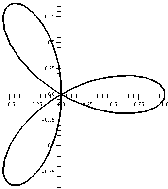
r=cos(3). Area inside one petal? Well, cos(3) "first" (going from 0 to 2Pi) is 0 when 3)=Pi/2. So we get half a petal by integrating from 0 to Pi/6. The formula is _A^B(1/2)r²d so this becomes (for the whole petal, we need to double):
2·(1/2)₀^Pi/6 cos(3)²d. How can we do this integral? Let's look at the formula sheet for the final exam.

On the formula sheet we are advised that A last link!
If you wish to see dyamically (!) how some roses are drawn (r=cos(3) and r=cos(4)) then
GO HERE but
Warning! the files are quite large, and may take a while to load.

"Standard issue" polar coordinates

An example and the problem with polar coordinates

Common restrictions on polar coordinates and the problems they have

Conversion formulas

Specifying regions in the plane in polar fashion

Graphing polar functions

A collection of examples

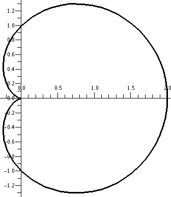
Let's consider r=3+sin(). Since the values of sine are all between -1 and 1, r will be between 2 and 4. Any points on this curve will have distance to the origin between 2 and 4 (the green and red circles on the accompanying graph). When =0 (the positive x-axis) r is 3. As increases in a counterclockwise fashion, the value of r increases to 4 in the first quadrant. In the second quadrant, r decreases from 4 to 3. In the third quadrant, corresponding the sine's behavior (decrease from 0 to -1) r decreases from 3 to 2. In all of this {in|de}crease discussion, the geometric effect is that the distance to the origin changes. We're in a situation where the central orientation is what matters, not up or down or left or right. Finally, in the fourth quadrant r increases from 2 to 3, and since sine is periodic with period 2Pi, the curve joins its earlier points. The picture to the right shows the curve in black. I'd describe the curve as a slightly flattened circle. The flattening is barely apparent to the eye, but if you examine the numbers, the up/down diameter of the curve is 6, and the left/right diameter is 6.4.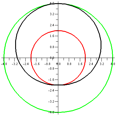
Now consider r=2+sin(). Again, the values of sine are all between -1 and 1, so r will be between 1 and 3. Any points on this curve will have distance to the origin between 1 and 3. We can begin (?) the curve at =0 when r=2, and spin around counterclockwise. The distance to the origin increases to r=3 at =Pi/2 (the positive y-axis). The distance to the origin decreases back to r=2 when =Pi (the negative x-axis). The curve gets closest to the origin when =3Pi/2 (the negative y-axis) when r=1. Finally, r increases (as increases in the counterclockwise fashion) to r=3 again when =2Pi. Here the "deviation" from circularity in the curve is certainly visible. The bottom seems especially dented.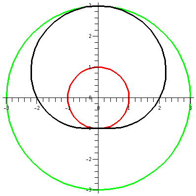
We decrease the constant a bit more, and look at r=1+sin(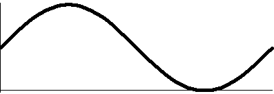). The values of sine are all between -1 and 1, so r will be between 0 and 2. The (red) inner circle has shrunk to a point. This curve will be inside a circle of radius 2 centered at the origin. We begin our sweep of the curve at 0, when r is 1. Then r increases to 2, and the curve goes through the point (0,2). In the interval from Pi/2 to Pi, sin() decreases from 1 to 0, and the curves moves closer to the origin as r decreases from 2 to 1. Something rather interesting now happens as travels from Pi to 3Pi/2 and then from 3Pi/2 to 2Pi. The rectangular graph of 1+sine, shown here, decreases down to 0 and then increases to +1. The polar graph dips to 0 and then goes back up to 1. The dip to 0 in polar form is geometrically a sharp point! I used "!" here because I don't believe this behavior is easily anticipated. The technical name for the behavior when r=3Pi/2 is cusp. This curve is called a cardioid from the Latin for "heart" because if it is turned upside down, and if you squint a bit, maybe it sort of looks like the symbolic representation of a heart. Maybe.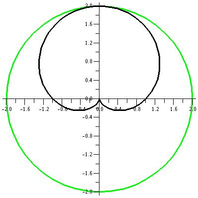
Here's the final curve we'll consider in this family: r=1/2+sin(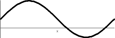). The values of sine are all between -1 and 1, so r will be between -1/2 and 3/2. The (red) inner circle actually had "radius" -1/2, and it consists, of course, of points whose distance to the pole, (0,0), is 1/2. When is 0, r is 1/2. In the first two quadrants, 1/2+sin() increases from 1/2 to 3/2 and then backs down to 1/2. In the second two quadrants, when is between Pi and 2Pi, more interesting things happen. The rectangular graph on the interval [0,2Pi] of sine moved up by 1/2 shows that this function is 0 at two values, and is negative between two values. The values are where 1/2+sin()=0 or sin()=-1/2. The values of satisfying that equation in the interval of interest are Pi+Pi/6 and 2Pi-Pi/6. The curves goes down to 0 distance from the origin at Pi+Pi/6, and then r is negative until 2Pi-Pi/6. The natural continuation of the curve does allow negative r's, and the curve moves "behind" the pole, making a little loop inside the big loop. Finally, at 2Pi-Pi/6, the values of r become positive, and the curve links up to the start of the big loop. This curve is called a limacon. The blue lines are lines with 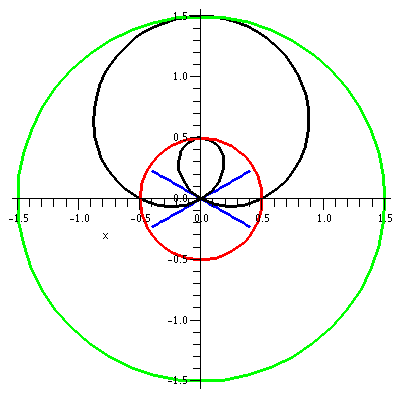=Pi+Pi/2 and =2Pi-Pi/6. These lines, for the values which cross the pole, are actually tangent to the curve at the crossing points.

More information about these curves is available here

Exponential?

Snails

Announcements
Teaching evaluations will be requested at the next class meeting.
Here is information about final exam, including review material, review sessions, and the date, time, and place of the examination.

Parametric curves
We begin our rather abbreviated study of parametric curves. These curves are a rather clever way of displaying a great deal of information. Here both x and y are functions of a parameter. The parameter in your text is almost always called t. The simplest physical interpretation is that the equations describe the location of a point at time t, and therefore the equations describe the motion of a point as time changes. I hope the examples will make this more clear.

Example 1
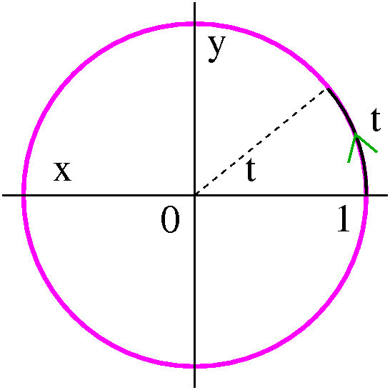
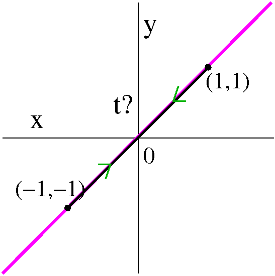
Suppose x(t)=cos(t) and y(t)=sin(t). I hope that you recognize almost immediately that x and y must satisfy the equation x²+y²=1, the standard unit circle, radius 1, center (0,0). But that's not all the information in the equations.

The point (x(t),y(t)) is on the unit circle. At "time t" (when the parameter is that specific value) the point has traveled a length of t on the unit circle's curve. The t value is also equal to the radian angular measurement of the arc. This is uniform circular motion. The point, as t goes from -infinity to +infinity, travels endlessly around the circle, at unit speed, in a positive, counterclockwise direction.

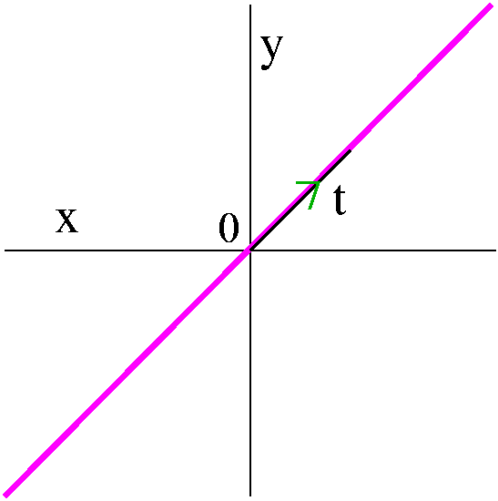
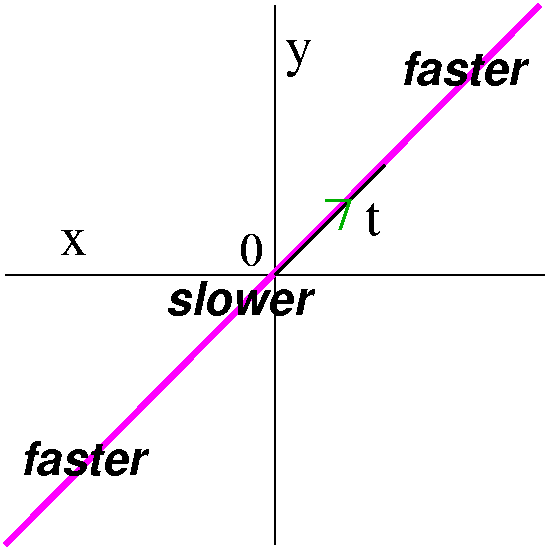
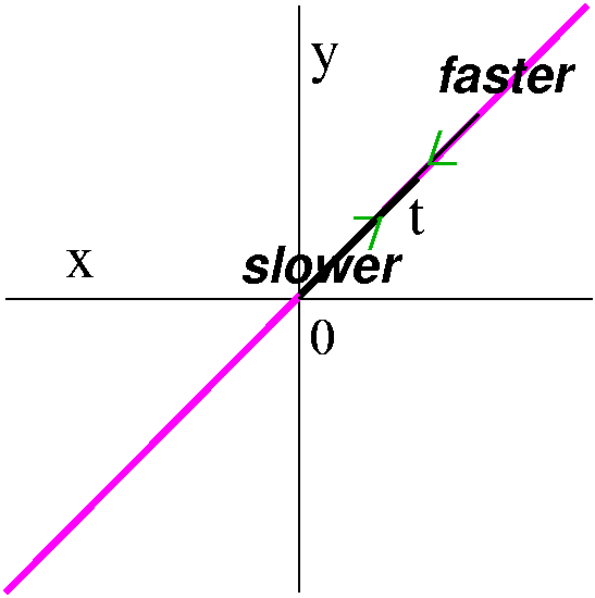
Example 2
Here is a sequence of (looks easy!) examples which I hope showed students that there is important dynamic (kinetic?) information in the parametric curve equations which should not be ignored.

x(t)=t and y(t)=t. Surely the "particle" travels on the main diagonal line y=x. The travel (remember, the domain unless otherwise limited, is all values of t which makes sense to the defining functions) is from lower left (third quadrant) to upper right, (first quadrant). Also I hope that you see the particle moves at uniform speed. This is uniform linear motion.
x(t)=t3 and y(t)=t3. The path of this point is also on the main diagonal line y=x. But the motion of this point, while in the same direction as the first example (from third to first quadrant), is very different. The difference is in the "clock". Try a few values of t. Between t=0 and t=1 we travel from (0,0) to (1,1). Between t=1 and t=2, we travel from (1,1) to (8,8). Just roughly, the distance changes from sqrt(2) to sqrt(98). That's a big change. The particle, near -infinity, travels fast. Then as t goes around 0, it is slower, and, as t gets very large positive, the particle moves faster.
Now let's consider the motion described by x(t)=t2 and y(t)=t2. Again, we can "eliminate the parameter". That rather grim phrase (if you read murder mysteries!) is what the text uses to describe getting rid of t by manipulating the two equations. Here we just realize that x=y. Much of the information about the motion of this point on the main diagonal is lost if we go to just y=x. The t2 means that both x and y must be non-negative. When t is large negative, the point is way up high in the first quadrant, and traveling towards the origin rather rapidly. It begins to slow, and then "stops" (!) but only "instantaneously" (!!) at (0,0) (when t=0). It turns around (how the heck does a particle "turn around"?) and begins to retrace its path, up towards the open end (??) of the first quadrant. As it travels, its speed increases. So this is really quite complicated motion, and very different from the first two examples.
The final example in this series is x(t)=cos(t), and y(t)=cos(t). Again, the path traveled by the point is on the main diagonal line y=x. But now the dynoamics are extremely different. Because cosine oscillates endlessly between -1 and +1, the motion of the point whose position is described by these equations is on the line y=x and only between (-1,-1) and (1,1). It moves back and forth between these points, completing a round trip in every time interval of length 2Pi. This is very different motion from the other examples.

Example 3

I considered x(t)=5cos(t)and y(t)=5sin(t). This is a slight variant of the very first example. Since x(t)/5=cos(t) and y(t)/5=sin(t), I "know" that the particle's path must be on (x/5)2+(y/5)2=1, so x2+y2=52, a circle whose center is (0,0) and radius is 5.

What if x(t)=5cos(t) and y(t)=3sint(t)? Then the trig identity gives (after elimination of the parameter) (x/5)2+(y/3)2=1 as the possible path of the point. This is an ellipse centered at (0,0). Its wider part (total length 1) is on the horizontal axis, as shown. The vertical extant of the ellipse is 6. So I attempted to create a moving image of this curve. I hope it is helpful to you. The parameterization is by central angle. Speed varies, and the point moves faster when it is farther away from the center. Planets move in ellipses with the sun at a focus. Planets generally more slower when they are farther away and faster when they are closer to the sun.

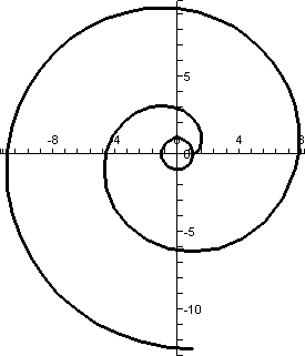
A bug drawing out a thread ...
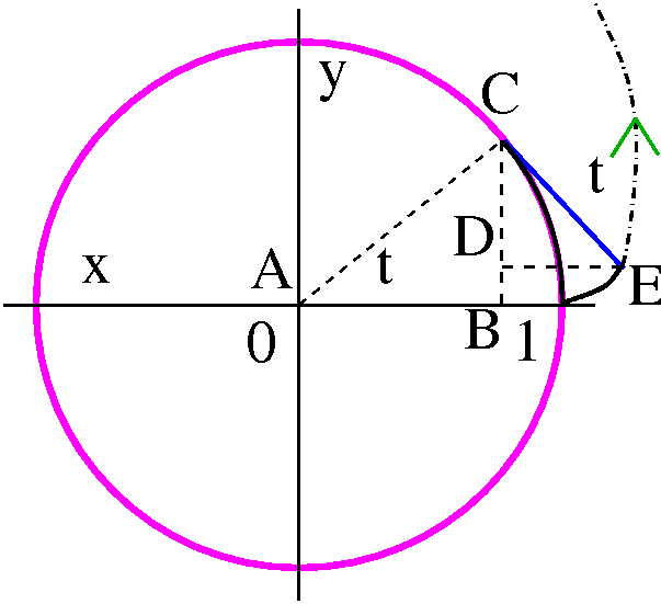Thread is wound around the unit circle centered at the origin. A bug starts at (1,0) and is attached to an end of the thread. The bug attempts to "escape" from the circle. The bug moves at unit speed.

I would like to find an expression for the coordinates of the bug at time t. Look at the diagram. The triangle ABC is a right triangle, and the acute angle at the origin has radian measure t. The hypoteneuse has length 1, and therefore the "legs" are cos(t) (horizontal leg, AB) and sin(t) (vertical leg, BC). Since the line segment CE is the bug pulling away (!) from the circle, the line segment CE is tangent to the circle at C. But lines tangent to a circle are perpendicular to radial lines. So the angle ECA is a right angle. That means the angle ECD also has radian measure t. But the hypoteneuse of the triangle ECD has length t (yes, t appears as both angle measure and length measure!) so that the length of DE is t sin(t) and the length of CD is t cos(t).

The coordinates of E can be gotten from the coordinates of C and the lengths of CD and DE. The x-coordinates add (look at the picture) and the y-coordinates are subtracted (look at the picture). Therefore the bug's path is given by x(t)=cos(t)+t sin(t) and y(t)=sin(t)-t cos(t).

t between 0 and 1	t between 0 and 10 Note the scale is changed!

Finally to the right is an animated picture of the bug moving. Maybe you can understand this picture better: maybe (!!).
This curve is more typical of parametric curves. I don't know any easy way to "eliminate" mention of the parameter. This seems to be an authentically (!) complicated parametric curve, similar to many curves which arise in physical and geometric problems. It has an official name. It is called the evolute of the circle. MORE TO COME IN THIS DIARY ENTRY.

Slopes of secant and tangent lines
Here we use a sort of Taylor approximation to get a useful formula for the slope of a line tangent to a parametric curve.

Tangents at the self-intersection

Length of a path

How useful is it?

Example

QotD
What is the state bird of New Jersey?
I am happy to report that about two-thirds of the registered students answer this question. More than half (barely!) reported the correct answer: the Eastern Goldfinch. New Jersey "shares" this state bird with Iowa. The next most common answer was Cardinal, which is the state bird for 6 other states. Some of the other answers were rather bizarre.

animate

Taylor's Theorem with Lagrange's form of the remainder
There is some number c between a and x so that f(x)=_j=0ⁿ[f^(j)(a)/j!](x-a)^j + [f⁽ⁿ⁺¹⁾(c)/(n+1)!]{(x-a)ⁿ⁺¹.

Yet another Taylor series example but different
Suppose f(x)=sqrt(x) or, if you wish, f(x)=x^1/2. Then f´(x)=(1/2)x^-1/2 and f⁽²⁾(x)=(1/2)[-(1/2)]x^-3/2 and f⁽³⁾(x)=(1/2)[-(1/2)][-(3/2)]x^-5/2, etc.

So this all looks "o.k." except there is one slight problem. I mentioned that most people like to apply Taylor's Theorem with a=0, because it just seems more computationally direct. In this case, if we want to construct Taylor polynomials with a=0, that is, polynomials such as T₃(x)=f(0)+f⁽¹⁾(0)x+[f⁽²⁾(0)/2]x²+[f⁽³⁾(0)/6]x³, we will have a difficult time because, for example, f⁽²⁾(x)=-(1/4)x^-3/2, and plugging in x=0 gives an expression involving division by 0. This is not good.

One possible workaround
"A workaround is a method, sometimes used temporarily, for achieving a task or goal when the usual or planned method isn't working."

What can we do here? Well, one "solution" is to choose another a. We should take a value of a which would make the Taylor polynomials easy to calculate. One choice is a=1 instead of a=0. Then the values of the derivatives, which all look like {One constant}x^{Some other constant}, become {One constant} because 1^{Some other constant} is 1. So if a=1 we get:
f(1)=1^1/2=1 and f⁽¹⁾(1)=(1/2)1^-1/2=1/2 and f⁽²⁾(1)=(1/2)[-(1/2)]1^-3/2=-1/4 and f⁽³⁾(1)=(1/2)[-(1/2)][-(3/2)]1^-5/2=3/8, etc.
We can use these numbers to "construct" our Taylor polynomials, but remember that the polynomials have (x-a)'s in them. So, for example, we would have
T₃(x)=f(1)+f⁽¹⁾(1)(x-1)+[f⁽²⁾(1)/2](x-1)²+[f⁽³⁾(1)/6](x-1)³=
          1+(1/2)(x-1)+[-(1/4)/2](x-1)²+[(3/8)/6](x-1)³=
          1+(1/2)(x-1)-(1/8)(x-1)²+(1/16)(x-1)³
(By the way, the next term is -(5/128)(x-1)⁴ so the coefficients are not as simple as the first few seem to be!)
So we could do this. People really do like to have a=0, so they frequently do something else, and it is this something else which is done in your textbook.

Another possible workaround
Instead of looking at the function f(x)=x^1/2 with a=1, move the function so we can still take a=0. So let us change the function to f(x)=(1+x)^1/2, and then:
      f(x)=(1+x)^1/2 so f(0)=(1+0)^1/2=1
      f⁽¹⁾(x)=(1/2)(1+x)^-1/2 so f⁽¹⁾(0)=(1/2)(1+0)^-1/2=(1/2)
      f⁽²⁾(x)=(1/2)[-(1/2)](1+x)^-3/2 so f⁽⁰⁾=(1/2)[-(1/2)](1+0)^-3/2=-(1/4)
      f⁽³⁾(x)=(1/2)[-(1/2)][-(3/2)](1+x)^-5/2 so f⁽⁰⁾=(1/2)[-(1/2)][-(3/2)](1+0)^-5/2=(3/8)
Now T₃(x) will be a polynomial centered at a=0.
      T₃(x)=f(0)+f⁽⁰⁾(0)(x-0)+[f⁽²⁾(0)/2](x-0)²+[f⁽³⁾(0)/6](x-0)³=
          1+(1/2)x+[-(1/4)/2]x²+[(3/8)/6]x³=
          1+(1/2)x-(1/8)x²+(1/16)x³.

Of course the polynomials we get are essentially the same as in the first workaround: we get the same sequence of coefficients, and have just replaced the x-1's by x-0's (that is, x's).

What happens?
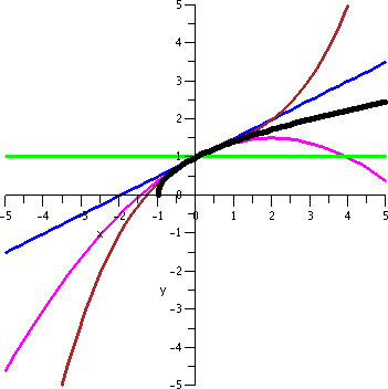
To the left is one graph of f(x)=x^1/2. The x-values are the interval [-5,5]. This is a bit silly, because the domain of the function is just [-1,infinity], so the graph is half of a parabola in black. What are the other curves? I have colored the curves to correspond to various formulas, so

• In black is f(x)=x^1/2 and f(4)=(1+4)^1/2=2.236.
• In green is T₀=1 and T₀(4)=1.
• In blue is T₁=1+(1/2)x and T₁(4)=1+(1/2)(4)=1+2=3
• In magenta is T₂=1+(1/2)x-(1/8)x² and T₂(4)=1+(1/2)(4)-(1/8)4²=3-(1/2)=2.5
• In brown is T₃=1+(1/2)x-(1/4)x²+(1/16)x³ and T₃(4)=1+(1/2)(4)-(1/8)4²+(1/16)4³=2.5+4=6.5.

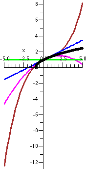
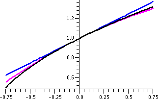
Here is another picture of the same curves. This is maybe a more honest picture. In the first picture, my window was [-5,5] in both the horizontal and vertical directions. Here I have let the vertical dimension be determined by the graphs of the functions, that is, what the ranges of the five functions are on [-5,5]. So you can see how badly the third degree Taylor polynomial makes things look.

Higher degree Taylor polynomials make things even worse for x's which are not in the interval from -1 to 1. So this is a much more subtle phenomenon than for sine or cosine or exponential.

sqrt(1.5)
Well, let's look at an example. Suppose I wanted to compute sqrt(1.5) using Taylor polynomials. By the way, this is definitely not realistic. Newton's method is much more efficient computationally. I could try x=.5 and f(x)=(1+x)^1/2 and n=3. I'm using n=3 because we already have T₃(x). So:
sqrt(1.5)=T₃(.5)+Error.
What is the error? Taylor's Theorem states that it is determined by f⁽⁴⁾(c)|x|⁴/4!. We already computed the third derivative, and it was f⁽³⁾(x)=(3/8)(1+x)^-5/2 so that f⁽⁴⁾(x)=-(15/16)(1+x)^-7/2. How big can this be in absolute value? Well, |-(15/16)(1+x)^-7/2|=(15/16)/(1+x)^7/2: the x-stuff is on the bottom. x ranges from a=0 to x=.5, Since the power is on the bottom, the 4^th derivative is decreasing. The largest it can be is at 0, so the largest |f⁽⁴⁾(c)| can be is (15/16). The other stuff, |x|⁴/4!, since x=.5, becomes (.5)⁴/4!=1/[16·24]=1/384. So the largest the absolute value of the error can be is (15/16)(1/384)=5/2048 which is about .0025. Notice also that the sign of the error is negative, so I bet that T₃(.5) will overestimate sqrt(1.5).

The "true" value of sqrt(1.5) is 1.224744871 and T₃(1.5)=1.226562500. The approximation error is -0.001817629, so the approximation is an overestimate, and the size of the error is about what I predicted.

So why do people study this?
People rarely use these approximations to compute specific values of square root. Newton's method is much more efficient. But they do use these ideas to think about square root. If |x| is small, then sqrt(1+x) is approximately 1+(1/2)x. This is an overestimate, and the size of the error will be about (1/8)x². If you need a better approximation, then I think when |x| is small, that sqrt(1+x) is approximately 1+(1/2)x-(1/8)x². The error will be about (1/16)x³ (positive error for x>0 and negative error when x<0).
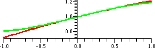
The graph to the right shows the three curves in the interval [-.75,.75].

A more intricate (and more realistic!) example
For example, suppose you needed to study a function like sqrt(1+sin[Ax]) for varying values of the parameter A but for small values of x. This sort of function might occur (does occur!) when you consider small motions of a pendulum. How would you expect the function to behave when A changes? Well, if x is small, Ax is small, and then sin(Ax) will be small. So I would guess that sqrt(1+sin[Ax]) would equal (approximately!) 1+(1/2)sin(Ax)-(1/8)(sin[Ax])² and then maybe I might think that sin(Ax) would equal (approximately!) Ax-(Ax)³/6 if x is small (first few times of the Taylor series for sine) so that sqrt(1+sin[Ax]) would equal (approximately!)
1+(1/2)[Ax-(Ax)³/6]-(1/8)[Ax-(Ax)³/6]²=1+(A/2)x-(A/12)x³-(1/8)(Ax)³
I am discarding terms of degree >3 because maybe for small x they won't matter too much. Then I bet that
sqrt(1+sin[Ax]) and 1+(A/2)x-[(3A³+2A)/24]x³ agree well when x is small. To the right is a graph of both curves when x=.5 and A is in the interval [-1,1]. Although this x is not too small, the agreement is still fairly good.
You might think such an example is silly, but it won't be silly if you are trying to adjust the parameter A (which might describe, fo0r example, some aspect of a material or a solution) to fit some requirement. Computing low degree polynomials is much easier than working with a composition of square root and sine.

How about (1+x)^1/3?
If f(x)=(1+x)^1/3, then:
      f(0)=1
      f⁽¹⁾(x)=(1/3)(1+x)^-2/3 so f⁽¹⁾(0)=(1/3)
      f⁽²⁾(x)=(1/3)[-(2/3)](1+x)^-2/3=-2/9(1+x)^-5/3.

I bet that (1+x)^1/3 is approximately 1=(1/3)x when |x| is small. The error or remainder is f⁽²⁾(c)x²/2 which is -1/9(1+c)^-5/3x².
If x=.05, then (1+.05)^1/3=1.016396357 and 1+(1/3)(.05)=1.016666667.
Now with c between 0 and .05, (1+c)^-5/3 will be at most 1 since again this is a negative power. I bet that the absolute value of the error will be at most (1/9)(.05)²=0.0002777777778.
Actually, 1.016396357=1.016666667+ERROR, and so ERROR=-0.000270310. The error is negative because of the sign in front of f⁽²⁾(c).

So 1+(1/3)x is a good approximation to (1+x)^1/3, with error roughly -1/9x². If I desperately wanted a better local approximation near x=0, I would use T₂(x), which would be 1+(1/3)x-(1/9)x², and I would expect the error (when x is small and positive) to be about (10/162)x³. Where did the 10/162 come from? Since f⁽²⁾(x)=-2/9(1+x)^-5/3, f⁽³⁾(x)=-2/9[-(5/3)](1+x)^-8/3=10/27(1+x)^-8/3. For x small and positive, this is at most 10/27. But we need to multiply this (for the Taylor error) by x³/3!=(1/6)x³. This gets us (10/162)x³.

Confession
I would not expect to use these ideas very often. But I should keep them in the back of my brain. When I want to approximate a weird function "locally" by a polynomial, the Taylor polynomials are really the first thing to try.

sqrt(17)
The square root of 16 is 4. What can be done to approximate sqrt(17)? Well, sqrt(16+1)=4sqrt(1+{1/16})=[approx]4(1+(1/32))=4.125, while the "true value" is about 4.123. Amazing! The correction will have a negative sign as we could predict (from -1/8x²).

(1+x)^m
Now (1+x)^m will be about 1+mx for small x, with correction [m(m-1)/2]x², etc.

Section 11.11, problem 11
The first part of the problem is "Use the binomial series to expand 1/sqrt(1-x²)." Page 773 of the text has "The Binomial Series". The result is:

If k is any real number and |x|<1, then
(1+x)^k=1+kx+[k(k-1)/2!]x²+[k(k-1)(k-2)/3!]x³+...
=_k=0^infinity(^k_n) for n>0 and (^k₀)=1.

Back to the solution of problem 11. Let me first take k=-1/2. Then the Binomial Theorem states: (1+x)^-1/2=1-(1/2)x+(3/8)x²-(5/16)x³+... (I did some arithmetic away from this record because I am getting tired of typing!). Now let me substitute -x² for x. The result is: (1-x²)^-1/2=1+(1/2)x²+(3/8)x⁴+(5/16)x⁶+...

The second part of the problem has this request: "Use part a) to find the Maclaurin series for arcsin(x)." I know that the integral from 0 to x of 1/sqrt(1-x²) is arcsin(x) (because arcsin(0)=0). So I will just integrate the answer to a) and make the integration constant equal to 0. Here is the result:
arcsin(x)=x+(1/6)x³+(3/40)x⁵+(5/112)x⁷+...

Comment If I wanted to compute values of arcsin, I would probably use this series. For example (10 digit accuracy) arcsin(.5)=0.5235987756 and the value of the seventh degree polynomial above when x=.5 is 0.5235258556 and that's not too far off for almost no work!

Section 11.11, problem 13
Part a) is "Expand (1+x)^1/3 as a power series." So this is the Binomial Theorem with k=1/3. Here are some terms (again, work done away from this page):
(1+x)^1/3=1+(1/3)x-(1/9)x²+(5/81)x³-(10/243)x⁴+...

Part b) asks for an estimation of "(1.01)^1/3 correct to four decimal places." I looked at the result above, and I think the series is alternating (the numbers f^(j)(0) change sign because (1+x)^{something negative} brings "down" a negative multiplier each time). Since the series is alternating, I can estimate the accuracy by just looking at the first omitted term. Hey, (5/81)(.01)³ will be less than .0001, so I bet that (1.01)^1/3 to 4 decimal place accuracy is 1+(1/3)(.01)-(1/9)(.01)².

Indeed, I am told (10 digit accuracy) that (1.01)^1/3 is 1.003322284 and 1+(1/3)(.01)-(1/9)(.01)² is 1.003322222. To me this is pretty darn good (8 digits!) for almost no work.

Section 11.11, problem 18
First, "Use the binomial series to find the Maclaurin series of f(x)=1/sqrt(1+x³)." I will break this into two steps. First I will use the Binomial Theorem with k=-1/2: (1+x)^-1/2=1-(1/2)x+(3/8)x²-(5/16)x³+... Then I will plug in (pardon me: "substitute") x³ for x: (1+x³)^-1/2=1-(1/2)x³+(3/8)x⁶-(5/16)x⁹+...

Part b) asks for the value of f⁽⁹⁾(0). Now I know that the coefficient of x⁹ in the power series will be equal to f⁽⁹⁾(0)/9!, so I look at the answer I just got, and see that this is -(5/16). Therefore f⁽⁹⁾(0) must be -(5/16)9!.

This number turns out to be -113,400, and you would not want to get it by directly computing the ninth derivative of 1/sqrt(1+x³) because that is

                18                 15                12               9
  678264862275 x     119693799225 x     31031725725 x     7161167475 x
- ---------------- + ---------------- - --------------- + --------------
            3 19/2            3 17/2            3 15/2            3 13/2
  512 (1 + x )       32 (1 + x )        8 (1 + x )        4 (1 + x )

                   6              3
        699238575 x     21432600 x      113400
     - -------------- + ----------- - -----------
               3 11/2         3 9/2         3 7/2
       2 (1 + x )       (1 + x )      (1 + x )

logarithm
The function ln has bad behavior at x=0, so people usually move the function in order to keep the series centered at 0 (people are stubborn!). Since ln(1+x) has derivative 1/(1+x), its series can be gotten by integrating the series for 1/(1+x)= (geometric!) 1-x+x²-x³+x⁴-x⁵+.... If we integrate the series we get x-(1/2)x²+(1/3)x³-(1/4)x⁴+(1/5)x⁵-x⁵+....+C. What is the correct value of C? When x=0, ln(1+x) becomes ln(1+0)=ln(1)=0, so C=0. And
ln(1+x)=x-(1/2)x²+(1/3)x³-(1/4)x⁴+(1/5)x⁵-x⁵+....

This series is not very useful for computational purposes. For example, when x=.9, the actual value of ln(1+.9) is 0.6418538862 but the 10^th partial sum of the series when x=.9 is 0.6261981044: one place accuracy, which is rather silly. There are other series, related to this one, which are used to compute values of ln.

Taylor's Theorem with Lagrange's form of the remainder
There is some number c between a and x so that f(x)=_j=0ⁿ[f^(j)(a)/j!](x-a)^j + [f⁽ⁿ⁺¹⁾(c)/(n+1)!]{(x-a)ⁿ⁺¹.

We used this in easy cases
The sine and cosine functions are very much the easiest functions. That's because we can estimate the M's as 1 (all the derivatives of sine and all the derivatives of cosine have their absolute values all bounded by 1). So the remainders-->0 and each function is the sum of its Taylor series for all x's.

"Computing" e^-.3
Let me describe how to compute e^-.3 with an accuracy of +/-.001:
e^-.3=T_n(-.3)+remainder.

Here x=-.3 and a=0 and we want to determine n so that (if possible!) the remainder has absolute value less than .001. Here the estimate we've been using for the remainder is M|-.3|ⁿ⁺¹/(n+1)!, and M is an overestimate of f⁽ⁿ⁺¹⁾(x) on the interval whose endpoints are a=0 and x=-.3. But the derivative is e^x (all of the derivatives are e^x!) and e^x is increasing on any interval. Therefore M is the value at the right-hand endpoint, and in this case this is e⁰=1. The error is less than 1(.3)ⁿ⁺¹/(n+1)!. The minus signs drop out because of the absolute value. The powers of the .3 on top make things smaller, and the factorials on the bottom, which grow quickly, also help to shrink the error. I think in class we just estimated that n=7 is sufficient. I was intentionally lazy. Here are the terms of this partial sum. -0.00002025000000

j=	Exact value	Decimal approximation
0	1		1
1	-3/10		-0.3000000000
2	-9/200		0.04500000000
3	27/80000		0.0003375000000
4	1		1
5	1		0.1012500000·10-5
6	81/80,000,000		0.1012500000·10-5
7	1		-0.4339285714·10-7

0.7408182191 0.7408182207

"Computing" e^.3

"Computing" e³

What happens in general ...

What is the exponential function?

Computing an integral
How could we compute ₀¹e^-x2dx?

Another series
Suppose, in a less-likely scenario, we have to find the first 5 non-zero terms of the Taylor series for (3+2x)e^(x3)

A curious collection of facts
I wrote parts of the table below, and added entries as I explained them. So, for example, I defined sinh(x) (hyperbolic sine of x, pronounced "cinch of x") as the difference (1/2)[e^x-e^-x]. To get the series for this function, I took the series for e^x and substituted in -x for x. The result has minus signs at the odd powers. The difference of the two series divided by 2 is the series shown. The function cosh(x) (hyperbolic cosine of x, pronounced "cosh of x") is the average of e^x and e^-x. Its series is half of the sum of the series for each of the pieces. When the pieces are summed, the odd powers cancel, and the result is what is shown.

The most intriguing (strange, weird?) entries in the table below occur as a result of Euler's Formula. If you are willing to accept that there is a number i whose square is -1, then something strange happens as you consider e^ix. Notice that the powers of i have this behavior:
      i¹=i and i²=-1 and i³=i·i²=-i and i⁴=i·i³=i·(-i)=(-1)(-1)=1 and ...
The powers of i repeat ever four times. Therefore
      e^ix=1+(ix)+(ix)²/2+(ix)³/6+(ix)⁴/24+...
      e^ix=1+ix-x²/2-ix³/6+x⁴/24+...
The even terms are exactly like the series for cosine, and the odd terms all have i, and except for that are like the series for sine. So:

Euler's Formula
eix=cos(x)+i sin(x)

Then because sine is odd and cosine is even, e^-ix=cos(x)-i sin(x). This gets the entries in the formula column for sine and cosine (add and subtract the two equations).

Function	Formula	Differential equation (actually, the initial value problem)	Power series
sin(x)	eix-e-ix ---------- 2i	y´´=-y y(0)=0 and y´(0)=1 Simple harmonic motion, init. vel. sol'n	x-x3/3!+x5/5!+...
cos(x)	eix+e-ix ---------- 2	y´´=-y y(0)=1 and y´(0)=0 Simple harmonic motion, init. pos. sol'n	1-x2/2!+x4/4!+...
sinh(x)	ex-e-x ---------- 2	y´´=y y(0)=0 and y´(0)=1	x+x3/3!+x5/5!+...
cosh(x)	ex+e-x ---------- 2	y´´=y y(0)=1 and y´(0)=0	1+x2/2!+x4/4!+...

Then I discussed ...
The responsibility of students to hand in work that is good. I referred specifically to writeups of the last workshop problem. I prepared an answer to this problem.
I remarked that workloads increase as students progress to more advanced courses, and that more sophisticated study skills were needed.
I returned the second exam.

April 2007 S M Tu W Th F S 8 9 10 11 12 13 14 15 16 17 18 19 20 21 22 23 24 25 26 27 28 29 30

We have six more lecture meetings, including today and excluding the exam day on April 11. I propose (subject to revision if something doesn't work!) to use this time in the following way: 3 lectures dedicated to explaining uses of Taylor's Theorem, 1 lecture devoted to parametric curves, and 2 lectures devoted to calculus in polar coordinates.

Here is a restatement of Taylor's Theorem. The vocabulary will be what's generally used when people discuss Taylor's Theorem.

Taylor's Theorem with Lagrange's form of the remainder
There is some number c between a and x so that f(x)=_j=0ⁿ[f^(j)(a)/j!](x-a)^j + [f⁽ⁿ⁺¹⁾(c)/(n+1)!]{(x-a)ⁿ⁺¹.