| Lecture date with link (as appropriate) |
Comments with links (as appropriate) | ||
| Monday, May 5 | I hope to discuss the derivation of the heat equation today. Most of this is available here. I hope to add material on the fundamental solution of the heat equation: K(x,t)=1/(4Pi t)3/2exp(-||x||2/(4t)) and on the "transmission speed" of heat, and thus its macroscopic suitability as a model. There are 76,200 google references for the phrase "fundamental solution of the heat equation"! | ||
| Wednesday, April 30 |
 I haven't bothered to keep up with this pseudo-diary, since
much of what I have done is a duplicate of last semester's
presentations. However, the discussion on flow boxes to illustrate
the definition of divergence is new, and I also promised an image of a
complicated surface. So here is a picture of Alexander's horned sphere
(what's inside of it?). More information about insides
and outsides is available.
| ||
| Monday, March 31 | A wonderful polar coordinate integral and computation of
(1/2)!. Change of variable in polar coordinates. | ||
| Thursday, March 27 | Conversion of double integrals to polar coordinates; the gravity of a flat earth. | ||
| Wednesday, March 26 | The instructor survived his experience. Please see the diary entry for last semester. A useful assertion was made: the existence of the double integral and the truth of Fubini's Theorem (conversion of double integrals into iterated integrals) holds not only for functions which are continuous in rectangles, but also for functions which have discontinuities on lower-dimensional sets. Several examples were done using this fact. This material is covered in section 15.3 of the text. I will ask students to do one homework problem from this section tomorrow in class. There will be opportunity for students to ask questions before the request. | ||
| Monday, March 24 | I reviewed Riemann sums, partitions, sample points, and the
definition of the definite integral for one variable. I pointed out a
scheme which would allow approximation of the definite integral with
an error bound for definite integrals of differentiable functions. We then extended integration to two variables, and described the formal setup for integrating a function defined over a rectangle in R2. This is section 15.1, the definition of the double integral. I even tried to estimate a definite integral of a "horrible" function over a rectangle. Now something new does come in: Fubini's Theorem asserts that under certain general circumstances, this double integral is equal to iterated (repeated) integrals in each of the variables separately. I then did a problem from section 15.2. | ||
|
Monday, March 10 Wednesday, March 12 | I worked on Lagrange multipliers. I mostly did examples much
like those done in the previous semester. Please see the lines to the
right. I gave out an analysis of two non-routine problems, along with
some pictures. We did several problems from 14.5 in preparation for the exam tomorrow. | ||
| Thursday, March 6 |
I discussed the definitions of {local|absolute|strict} m{axi\ini}ma. (That's a total of six definitions!) I stated the second derivative test for functions of two variables today and tried to do two examples. Let me tell you about them.
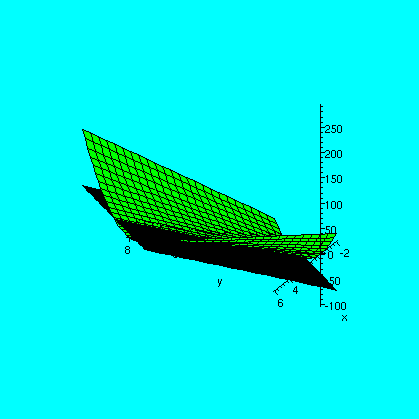
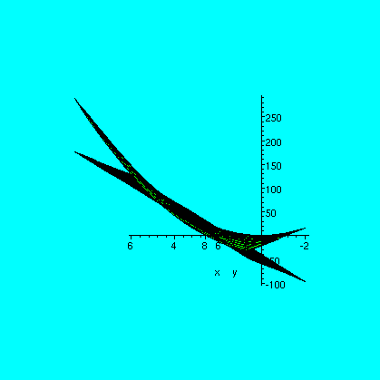
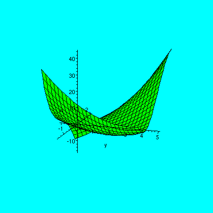
In fact, this was a problem on my first exam in Math 291 in the fall 2002 semester, and a complete solution is available. It turns out that Euler was wrong. One of the critical points is a local minimum and the other is a saddle. The picture to the right is the output from Maple of the following sequence of instructions:
with(plots):
V:=x^3+y^2-3*x*y+(3/2)*x;
                           3    2
                     V := x  + y  - 3 x y + 3/2 x
plot3d(V,x=-2..3,y=-1..5,color=red,axes=normal);
If you try this in a Maple window, you should be able to rotate the
graph enough to perhaps convince yourself that the assertion about the
critical points is possibly true. Graphs of surfaces can be subtle.
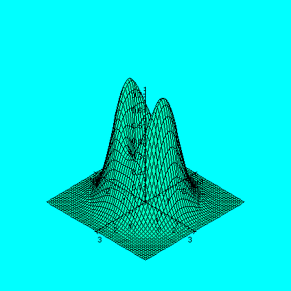
Example 2 If
f(x,y)=(x2+2y2)e-x2-y2,
locate and characterize (max, min, saddle) the five critical points of
f.
So I asked Maple to do the work.
solve({diff(W,x),diff(W,y)});
  {y = 0, x = 0}, {y = 0, x = 1}, {y = 0, x = -1}, {y = 1, x = 0},{x = 0, y = -1}

H:=simplify(diff(W,x$2)*diff(W,y$2)-(diff(W,x,y))^2);
                  2      2        2  2       4  2       2  4
  H := -4 exp(-2 x  - 2 y ) (-26 x  y  + 10 x  y  + 16 x  y  - 2

               2       2       4      4      6      6
         + 14 y  + 11 x  - 24 y  - 9 x  + 8 y  + 2 x )

eval(subs(x=0,y=0,H));
                                  8
eval(subs(x=0,y=0,diff(W,x$2)));
                                  2
According to the second derivative test, I have verified that H has a
local max at (0,0) with this computation. The next topic is constrained max/min in several variables. Here the 1-dimensional case is considerable easier than the several variable case. So first I tried to review the 1-dimensional case. Suppose we are given a function of 1 variable on the interval [a,b]. Where should we search for the absolute maximum and the absolute minimum of the function? This is a well-known topic in 1-variable calculus, and most students have an almost Pavlovian response: look for critical points inside the interval (where the derivative is 0 or doesn't exist). Examine the values of the function at these points, and compare the values at the end-points of the interval. This list of values will contain the max and the min of the function.
Of course, that might bring up the question, "Does a function on a
closed, bounded interval always attain its maximum and minimum?" Here
are a few examples. The missing word here is continuity. A continuous function on [a,b] always attains its max and its min. For many "nice" functions, then, checking to get the max and min means checking a short list of interior critical points and the endpoints, a and b. In several variables the situation is dominated by the following theoretical idea:
Theorem Suppose we look at a region in Rn which is
bounded (that is, can be put inside a large ball) and which also
contains all of its boundary. Then any continuous function on the
region must attain its maximum and its minimum. | ||
| Wednesday, March 5 | I first discussed Taylor's Theorem in one variable. A
discussion similar to this was done last semester and I refer to
that.
I then tried to discuss Taylor's Theorem in two variables. This calls
for some imagination. I wanted to consider F(a+h,b+k) and did it by
looking at the one-dimensional "slice" function, f(t)=
F(a+ht,b+kt). So f(0)=F(a,b) and f(1)=F(a+h,b+k). To apply the
one-variable Taylor's Theorem, I need to compute f'(0) and f''(0),
etc. So with some luck, using the Chain Rule very carefully, we did
this: f'(t)=D1F(a+ht,b+kt)h+D2F(a+ht,b+kt)k so that f'(0)=D1F(a,b)h+D2F(a,b)k f''(t)=D1D1F(a+ht,b+kt)h2+D2D1F(a+ht,b+kt)hk+D1D2F(a+ht,b+kt)kh+D2D2F(a+ht,b+kt)k2. f''(0)=D1D1F(a,b)h2+2D1D2F(a,b)hk+D2D2F(a,b)k2. The last equation results from the equality of "mixed partial derivatives" and the commutitivity of multiplication (hk=kh). In fact, one can now see the general pattern. The same formation rule as comes into effect for the Binomial Theorem occurs here. Every time we differentiate a derivative of F, the Chain Rule takes effect. It "spits out" an h with every D1, and a k with every D2. The binomial coefficients occur because the rule of formation is the same as in Pascal's Triangle. In any case, what we have is (when t=1):
Taylor's Theorem, in a sort of two variable version): I very quickly reminded people of what local max and min were, and the fact that such must occur at critical points. Again, please see last semester's notes. A critical point occurs where the gradient is 0 or where the gradient doesn't exist (such can happen: the vertex of a cone, for example). But if we are at a point where grad F = 0, how can we tell if we are at a local max, a local min, or a saddle?
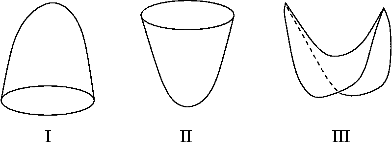 < <
Sometimes you can just "see" it. For example, we considered the almost silly example a44+b144+c20+d100+e3. The only critical point of this function is (0,0,0,0,0) (the only point where all of the 5 first partials are 0), which must be a saddle because of the odd degree in the variable e.
But let us look at a classical example, two variables. Here a critical
point (if the function is differentiable) is where the two partial of
F are 0. So let us assume that is true at the point (a,b). How does
the behavior of the second-degree Taylor polynomial influence the
local "geometry" of the graph of the function. I restricted myself to
initially asking how to get the picture II, a local minimum.
The second-degree Taylor polynomial is: Wow! We have verified/motivated part of what is called the second derivative test for two variables. I will discuss this further tomorrow, but: if A>0 and if AC-B2>0, then the function has a local maximum. Wow! Of possible interest is this web page from Georgia Tech, discussing Taylor's Theorem in two variables. I tried to find a "dictionary" of pictures on the web of what happens in two variables when one considers cubic polynomials but I haven't been able to find a good link. I will continue looking. The pictures can get quite complicated. | ||
| Monday, March 3 | I first explained a part of a Maple dialog:
showtime(true); Turns on timing information.
vv:=x^2*arctan(exp(sin(3*y))); Defines a function.
                        2
                       x  arctan(exp(sin(3 y)))
time = 0.00, bytes = 62706Time/storage needed.
vvd:=diff(vv,y$50): Asks for 50 y derivatives.
time = 4.19, bytes = 114534450"Expression swell."
diff(vvd,x$3); Three x derivatives.
                                  0
time = 0.28, bytes = 3794046
diff(vv,x$3); The three x derivatives first.
                                  0
time = 0.00, bytes = 6086
off; Turns off timing information.
So the order that derivatives are taken doesn't seem to matter. This
is called Clairaut's Theorem in your text. If partials exist
and are continuous, then the order in which they are taken does not
matter (at least theoretically!). Of course, what I tried to show
above is that such things might well matter computationally! The
verification of Clairaut's Theorem is in an appendix in your text, and
uses the Mean Value Theorem a few times. I also tried to give an
analogy with taking marginal "things" with respect to different
variables on a spreadsheet, but I am not sure I was too successful.Then I discussed traveling through a nebula in a rocket ship, and the temperature that was record, and the rate of change of the temperature. The most important chain rule computation is to "decouple" the effect of the nebula's temperature change and the rocket ship's travel. Discussion similar to what we did today is recorded here. | ||
| Thursday, February 27 | Much the same as the corresponding meeting the previous
semester. The first exam will be in two weeks from this class. Review material and other information will be handed out next week. | ||
| Wednesday, February 26 | Please look here for a discussion fairly
similar to what I did today. It is complicated stuff, and really
discussed some material which does not occur in 1-dimensional
calculus. Applications include "linearization" and equations for the tangent plane.
I tried to find an equation for a plane tangent to
z=4x2+3xy when x=2 and y=4 (there z=40). The normal vector
is supposed to be -dz/dxi-dz/dyj+k.
I would like to
show you that what I found algebraically "looks" correct. So here are
the output of some Maple commands. First, I typed
| ||
| Monday, February 24 | 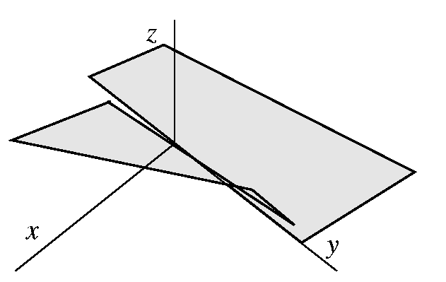 I remarked
that this week students should read and do problems in sections
14.1-14.5. Please. I remarked
that this week students should read and do problems in sections
14.1-14.5. Please. Example I wanted to do one more example about continuity, and it will be a bit more complicated than the others. The example is the following: f(x,y)=2x+3y if x>=0 and f(x,y)=0 for x<0. The picture shown here is an effort to graph this function, which sort of looks like two mutually tilted half planes. There is half a plane (where z=0) over the "left" half of the xy-plane, and a tilted plane (part of z=2x+3y) over the right half of the xy-plane. I asked where this function should and should not be continuous. We decided that it would be continuouis where x>0 and where x<0. On the line x=0, it would not be continuous everywhere except (0,0). We first explored what happened at (-3,7). In order to verify that f is continuous there, we wanted to restrict input values so that |f(x,y)-f(-3,7)| would be small. Well, since f(-3,7)=0, the simplest restriction would be one which would guarantee that f(x,y) also would be 0. But for that to be true, (x,y) would have to be in the left half-plane, where x<0. So the input tolerance, H, should be 3. Then any point (x,y) of R2 inside the circle of radius 3 centered at (-3,7) would have to be in the left half-plane, where x<0, so f(x,y)=0. Thus if we always take H=3, then |f(x,y)-f(-3,7)|=0 and this is less than any positive K. That's pretty easy. In fact, to show that f is continuous at (x0,y0) where x0<0, just take H=|x0|, and a similar logic applies to show that |f(x,y)-f(x0,y0)|=0<K for any positive K. This is definitely the easiest case. Then we looked at (3,7). Here and at nearby (x,y)'s, f(x,y) is given by the formula 2x+3y. We would expect that the correspondance we considered last time (take H=(1/sqrt(13))K) would play some part. It does, but the logic is a bit tricky. In order to apply the previous result, we need to be sure that every point inside the circle with radius H is in the right half-plane (mirror image of the previous consideration!) But that means here that H should never be bigger than 3. So, golly, H should be the minimum of 3 and (1/sqrt(13))K: H=min(3,(1/sqrt(13))K). There was a slight amount of discussion about min(A,B). I defined it by the following: min(A,B)=B if A>=B and =A if A<B. I also observed that min(A,B)=(A+B-|A-B|)/2 if this "formula" pleases you (?). There is a similar formula for the function max. Anyway, if the distance from (x,y) to (3,7) is less than H, then x>0, so f(x,y)=2x+3y. Then |f(x,y)-f(3,7)| is covered by the discussion last time, so that this difference is less than (1/sqrt(13))K·sqrt(13)=K, and we have verified continuity. Indeed, if (x0,y0) is in the right half-plane (so x0>0) then the specification H=min(x0,(1/sqrt(13))K) for the input tolerance will guarantee the output will be within K of f(x0,y0). What happens when x=0 is more subtle. We looked first at (0,7). Here we suspected f was not continuous. We computed f(0,7)=21. Mr. McGowen suggested that if we tried K=20, we would not be able to find any H which would guarantee "if ||(x,y)-(0,7)||<H, then |f(x,y)-f(0,7)|<K" (that is, 20). In fact, if H>) (as it is supposed to be) then (-H/2,7) will be inside the circle, and since -H/2<0, f(-H/2,0)=0 so that |f(x,y)-f(0,7)|=|0-21| which is not less than 20, and we have shown that the definition of continuity cannot be fulfilled. This "negation" argument is quite complex logically. It needs to be thought about. And the specification of K=20 is very neat, of course. I did not look at the lack of continuity of f at (0,y) (with y not 0), generally. The next part was worrying me!
f is continuous at (0,0). Given an "ouput" tolerance K>0,
how should we specify H? Here we decided that H=(1/sqrt(13))K. We must
analyze |f(x,y)-f(0,0)|. Since f(0,0)=0, we don't need to worry about
the (x,y)'s with x<0, because then f(x,y)=0, so
|f(x,y)-f(0,0)|=0<K always. But when x>=0, we need "yesterday's
result (the one that needed the Cauchy-Schwarz inequality), and that
will actually verify what we want.
Then we discussed differentiability. There is similar material here and here. Please look at these
entries.
| ||
| Thursday, February 20 | Stirling's formula allows one to approximate
factorials. Here's a
link with fairly readable exposition. One version of the formula
is: For large N, N! is approximately (N/e)^N*sqrt(2*Pi*N). This is a really handy fact. For example, Maple tells me in another window that the exact value of 100! divided by the approximation above (with N=100) is about 1.000833661 -- quite close to 1. Stirling's formula can be obtained by considering an improper integral: int0infinity xn e-x dx which equals n!. The equality is a nice exercise using mathematical induction and integration by parts. Much more than almost anyone would want to know about binomial coefficients is just a click away! Mr. Bergknoff gave a nice presentation of problem #4 of workshop #2. This is an intricate problem, and I thank him for his effort. After this I tried to give some background on the problem. Now how about continuity? Consider the following statement statement
Example Suppose f(x,y) assigns the number 1 if (x,y)=(0,0) and
otherwise its value is 0. Where is f continuous and where is f
not continuous? What about at other points? I first looked at (3,4). Well, if we get (x,y) close to (3,4) (what does "close" mean?) then probably f(x,y) and f(3,4) are both equal to 0, so that |f(x,y)-f(3,5)| will be 0 which is certainly less than ... well, less than any output tolerance K. Wow! So the K won't matter here, but a good choice of H is important. That is, we want H so that if sqrt((x-3)2+(y-4)2)<H, then f(x,y) will be 0. But the only way f will not be 0 is if (x,y)=(0,0). So we need to choose H so that (0,0) is "avoided". Here, with (3,4), "clearly" (well, almost clearly if you take the distance to (0,0)!) if H=5, we will avoid (0,0). More generally, I would like to prove that f is continuous at (x0,y0) when (x0,y0) is not (0,0). Well, if I choose H=sqrt(x02+y02), then H is positive (since the point is not (0,0)!) and then |f(x0,y0)-f(x,y)|=|0-0|, and this will always be less than any positive output tolerance, K.
Example I considered the more complicated function f(x,y)=2x+3y
and asked where this function is continuous. Almost everyone agreed
that it would be continuous at every point. I decided to try to verify
that the function was continuous at (4,5), so f(4,5)=23. Therefore I
need to check the following intricate logical statement: If we understand sufficiently, we can now see how to prove that this f is continuous at any point (x0,y0). Given a K>0, the same choice of H which work at any point. So this function is actually in a certain logical sense "simpler" than the previous example, where H needed to change from point to point. We'll do more next time, before moving on to derivatives. | ||
| Wednesday, February 19 | Again discussed limits. One idea I tried to suggest is
analyzing functions by "reducing dimension". One way is with contour
lines, and another way is by slicing. We looked at a sequence of
increasingly frustrating examples. The idea is to contrast the
two-dimensional limit of f(x,y) as
(x,y)-->(x0,y0) with the existence of various
1-dimensional limits. So we might look at the limit as t-->0+ of x=x0+at and y=y0+bt for various values of a and b: these are one-dimensional slices at various "angles". If a=0 this is the slice with only y "moving" and if b=0 this is the slice with x "moving". If the two-dimensional limit exists, then the one-dimensional slice limits must all exist and must all be the value of the two-dimensional limit. But we saw that there are examples of functions with two-dimensional domains whose slices had various different values, and there are even examples of functions whose one-dimensional limit slices all exist and all have the same value, but which do not have a two-dimensional limit. So things can really be weird. Please look at the diary entries here and here. There are Maple pictures in each, and each picture is accompanied by the Maple command which produced it. | ||
| Thursday, February 13 | I again stated the exact definition of limit and worked with
it a bit. This material is covered more or less, here. We also analyzed the
alien limit problem and decided that the limit of f(x) (after the
values are changed) always exists, and is always x. To
me this fact is not totally obvious. Then I discussed graphs of functions whose domains are in R2 and whose ranges are in R. The link just given has Maple pictures and commands which may prove useful. Students should look at them. I began the study of limits in R2, and contrasted the 2-dimensional limits with limits of "slices" of functions, where only one of the variables is allowed to change and the others are fixed. Examples included the function which is always 0 for (x,y) in R2 except for (0,0) where it is 1, and the function which is always 0 for (x,y) in R2 except for where xy=0 (the coordinate axes) where it is 1. I will continue with further examples next time. | ||
| Wednesday, February 12 | Mr. Brown presented problem 3 of workshop 3 at the board. I
thank him for his efforts. I tried to encourage people in this rather small class to
I presented problem #4 of workshop #3 because no students did it, and I think that it is irritating enough to be useful to see. I did some problems from chapter 13. A review of limits. I stated the limit definition for real-valued
functions of one real variable:
I posed the following question for students to think about:
Question for tomorrow For which numbers a does
limx->af(x) exist, and what is the value of the limit for
those numbers?
| ||
| Monday, February 10 | I stated a general theorem about curves being determined
(roughly) by their curvature and torsion, and then remarked that was
quite difficult to determine interesting or useful "properties" of the
curve from just this information. For example, although the theorem I described was first proved around 1850 (actually, a little bit later), a useful application describing a necessary condition for a closed curve to be a knot was only obtained about a century later. This is a result called the Fary-Milnor Theorem, and states that a curve whose total curvature (integrate the curvature around the whole curve, using an idea of integration over a curve which we will see later in the course) is less than 4Pi must be unknotted. There has, in fact, been much more "progress" in recent years. Since detailed knowledge of space curves has turned out to be important in robotics, control theory, material science, and molecular biology, lots of new things have been studied. I did some problems from chapter 12. | ||
| Thursday, February 6 | Much as I did it last semester. I didn't quite finish, though, so I will have more to say Monday. | ||
| Wednesday, February 5 | I computed a simple example of a tangent line to a curve. I
also mentioned that actually "computing" the arc length of a curve by
nice antiderivatives would likely fail much of the time. The balance of the lecture duplicated most of what the link has, except for the last few sentences, which I will begin with next time. |
 Example 1 "Leonhard Euler (1707--1783)
was a great and very prolific
mathematician. He published Institutiones Calculi
Differentialis (Methods of the Differential Calculus) in 1755.
It was an influential text, and was the first source of criteria for
discovering local extrema of functions of several variables. In it
Euler investigated the following specific example:"
 I tried another example, which I had found in a calculus book.