| Date | What happened | ||||||||||||||||||||||||||||||||||||||||||||||||||||||
|---|---|---|---|---|---|---|---|---|---|---|---|---|---|---|---|---|---|---|---|---|---|---|---|---|---|---|---|---|---|---|---|---|---|---|---|---|---|---|---|---|---|---|---|---|---|---|---|---|---|---|---|---|---|---|---|
| 11/20/2002 | We discussed Green's Theorem. I first proved Green's Theorem for the unit square in R2. Here I started with the double integral of Qx-Py dA over the unit square S in the xy-plane: points (x,y) with 0=<x<=1 and 0=<y<=1. We decided that the best way to make sense of this was to convert it into an iterated integral. But the choice between dx dy and dy dx was not easy. In fact, the best thing was to split up the double integral and treat each part differently. Therefore: int intS (unit square)Qx-Py dA= intx=0x=1 inty=0y=1Qxdx dy - inty=0y=1 intx=0x=1Pydy dx= (using the Fundamental Theorem of Calculus, in the first integral with respect to x and in the second integral with respect to y) inty=0y=1 Q(x,y)]x=0x=1dy - intx=0x=1 P(x,y)]y=0y=1dx= intx=0x=1 Q(1,y)-Q(0,y) dy - inty=0y=1 P(x,1)-P(x,1) dy= inty=0y=1Q(1,y) dy-inty=0y=1Q(0,y) dy-intx=0x=1P(x,1) dx+intx=0x=1P(x,0) dx
So we have proved Green's Theorem for the square. The other conventional model situation is the circle. I decided to try an example here. The example I used is P(x,y)=(-y)/(x2+y2) and Q(x,y)=P(x,y)=(x)/(x2+y2). This is a wonderful example. Both Py and Qx are (y2-x2)/(x2+y2), the same thing. So Qx-Py is 0. But then we computed Pdx+Qdy over the unit circle using the parameterization x=cos(theta) and y=sin(theta) with 0=<theta<=2Pi. Amazingly, lots of -'s cancel out, and the integral (the "work done") is 2Pi. One possible corollary of this is 0=2Pi. I rather think that we have not understood Green's Theorem correctly. In fact, the hypotheses of Green's Theorem are very important.
Hypotheses of Green's Theorem
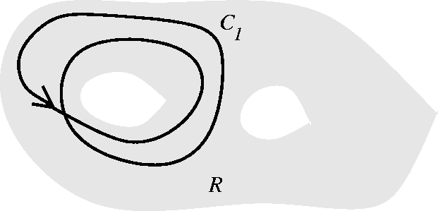
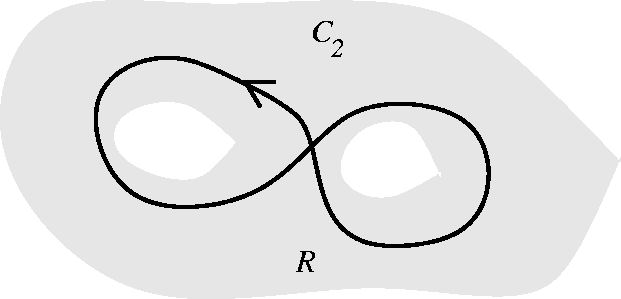
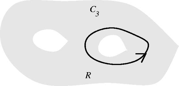
This specific Pdx+Qdy is a mathematical model for a unit charge at (0,0) if we are dealing with electricity, say. If we want to deal with Pdx+Qdy as modeling fluid flow, then Pdx+Qdy is actually a source at (0,0) and the velocity is away from the source at the origin. A harder problem, from traditional physics Suppose we're given a region in the plane with two holes in it, as shown. I'll call the left-hand hole, #1, and the right-hand hole, #2. Suppose I have two functions P(x,y) and Q(x,y) which are defined in this region (and you only know about their values in this region, not anywhere else!) with these properties:
Here we see that the integral over C1 is twice around hole #1, so the integral around hole #1 is 5. Note that we can change the shape of the curve a little bit and there will be no change in the line integral, because, as long as the change in shape takes place inside the region where we know that there is no net change in the integral (using Green's Theorem). The integral over C2 tells us that the integral over hole 1 - integral over hole 2 is 3. But then the integral over hole 2 must be 2, so that is the answer to the question. A simply connected domain is one which has no holes. The inside of a rectangle or the inside of a circle is a simply connected domain. If you "puncture" a disc (take out, say, the center) the result is not a simply connected domain. One important fact is as follows: if Py=Qx in a simply connected domain, then Pi+Qj is conservative and has a potential. This does not have to be true if the domain is not simply connected. The next major task in the course (and the last one one, actually) is to see what results there are corresponding to Green';s Theorem in three dimensions. The technical tool replacing line integrals will be surface integrals. | ||||||||||||||||||||||||||||||||||||||||||||||||||||||
| 11/18/2002 |
We investigated the relationship of the following ideas:
gradient/conservative vector fields <==> path independence <==> work
over closed
curves is 0 <==>construction of a potential Well, this is correct, but since the material is, both theoretically and for practical applications, among the most important in the course, perhaps I should write more. We saw last time that if we take f(x,y) and consider its gradient: fxi+fyj (so P(x,y)=fx and Q(x,y)=fy) then the line integral of P dx+Q dy is equal to f(END OF C)-f(START OF C). This was an application of the chain rule in 2 variables together with the Fundamental Theorem of Calculus in 1 variable. Therefore the value of the integral does not depend on the path connecting the two points: we say that P dx+Q dy is path independent. Indeed I carelessly drew a path connecting the START with the END which crossed itself: the work done on such a path is the same as on any simple curve. Mostly in this course the curves I'll draw will be simple curves. But we actually went on: a closed curve is one whose START=its END. We saw that if P dx+Q dy is path independent then its integral (the work done) over any closed curve must be 0. I think I then wrote down an example which was supposed to be absurd, something like f(x,y)=cosh(x2+x*sin(y3)) so the associated gradient is sinh((x2+x*sin(y3))*(2*x+sin(y3)i+is sinh((x2+x*sin(y3))*x*cos(y3)*3*y2j and then "clearly" (not!) the work done for this force around any closed curve is 0. f is the potential for this Pdx+Qdy. Note again that this f is not unique: you can modify it by adding or subtracting a constant. A major problem is the converse, logically, of these results. My on-line dictionary gives me this for the definition of converse: [Math.] a theorem whose hypothesis and conclusion are the conclusion and hypothesis of another. Here I am more interested in understanding the following question: suppose I tell you that Pdx+Qdy is, say, path independent, or, equivalently, that the integral of this over ALL closed curves is 0 (you can see this is equivalent by cutting up a closed curve into two pieces, and reversing the orientation on one of the pieces to get two closed curves, etc.). Then, given this information, how can we "construct" or evaluate a potential f for Pdx+Qdy. We had quite a lot of discussion about this. So here is a recipe we came up with:
How can we find f(x,y) algebraically given P and Q? What people might do is antidifferentiate. I think I used the following example in class: we assume that Pi+Qj is conservative, where P(x,y)=x2sin(y2) and Q(x,y)=x3y2 cos(y3)+y7. What is f? I integrated P with respect to x, so anything involving y is just an elaborate constant. Therefore f(x,y)=(1/3)x3sin(y3)+Constant1(y), where Constant1(y) might involve some function of y. I integrated Q with respect to y, so anything involving x is just an elaborate constant. Therefore f(x,y)=(1/3)x3sin(y3)+(1/8)y8+Constant2(x), where Constant2(x) might involve some function of x. It is important to understand the following remark: the expressions in green are two different representations of the function f(x,y). Both are correct. In order to indicate most clearly what the algebraic structure of f(x,y) is, use both representations: match the information. The (1/8)y8 in the second expression is "buried" in the Constant1(y) of the first expression. I don't think there are other "buried" expressions, and the only thing which can still be a mystery is only a "true" (no x or y!) constant. So, in fact, f(x,y)=(1/3)x3sin(y3)+(1/8)y8+C where C is a constant (whose specific value is related to the choice of "ground state"). Notice that when we evaluate line integrals, we will have f(END)-f(START) and the C's drop out: the ground state doesn't matter to this "potential difference". So if you are just interested in evaluating line integrals you don't need to pay much attention to the C's. However there will be other times that a choice of C matters. I tried another example, something like P(x,y)=x3y2 and Q(x,y)=x5y4 and after some discussion we decided that this just didn't work. In fact, there is no potential for this Pdx+Qdy. We had tried integrating (well, really, antidifferentiating) and couldn't get the two "representations" to agree. Also I asked if there might be a faster way to check if Pdx+Qdy were path independent (yes, we could write a list of all closed curves, evaluate the work around all closed curves, and see if it is 0, but that list would have to be very, very, very long!). Usually differentiation is a lot faster than integration. So if you notice the following string of implications:
I remarked that this result allows you to exchange a line integral for a double integral or the other way around. I challenged you with the following question: suppose a race car drives over a closed race course (a simple closed curve). Is it possible to determine from information the race car has the area enclosed by the race course? The area is the double integral of 1. Can we choose P and Q to get 1 in the double integral in Green's Theorem? P=1 and Q=x were suggested. In fact, there are many possible choices, like Q=42 and P=-y and ... So we can determine what goes on inside from boundary data. This and other things (to follow) are amazing. The area question was actually the motivation for the design of an instrument called the the planimeter. This link, to a webpage of Professor Robert L. Foote of Wabash College, includes moving images and pictures of actual planimeters. | ||||||||||||||||||||||||||||||||||||||||||||||||||||||
| 11/14/2002 | I prepared fairly careful notes, but they seem to have been
stolen away by evil spirits, so I must use memory to reconstruct
... I began by writing things which are in the textbook. That is, I wrote on the board the definition of line integral: intCf(x,y) ds using a parameterization: intt=STARTt=END f(x(t),y(t)) sqrt((dx/dt)2+(dy/dt)2) dt, where (x(t),y(t)) is a parameterization of C and START is the beginning time of the parameterization and END is the ending time of the parameterization. I then remarked that the most important kinds of line integrals occur with work, and wrote the text's intC F·dr which was intCF·r'(t) dt where r(t) is the position vector and F is the force field. Then r' is the velocity vector, which can be written as (ds/dt)T where T is the unit tangent vector. Putting things back together, and noticing that the one-variable chain rule implies (ds/dt) dt=ds, we see that the work integral actually is intCF·T ds. Wow! Now Flux, which I wasn't supposed to talk about yet, is intCF·N ds. This is actually the net flux, (fluid in) - (fluid out), through the curve. If F(x,y)=A(x,y)i+B(x,y)j, then the integral above, when we put in a parameterization, becomes intt=STARTt=END(A(x(t),y(t))(dx/dt)+B(x(t),y(t))(dy/dt)) dt, because all of the square root stuff cancels out. This is frequently abbreviated as intCA(x,y)dx+B(x,y)dy. The object to be integrated is sometimes called a differential form (it is not called this in your book!). I did some examples to try to show some neat properties of line integrals. So if the F were x2i+3xyj and if the C were the straight line segment from (0,0) to (2,1), I computed the work. Here I used the parameterization x=t so dx=dt and y=(1/2)t so dy=(1/2)dt with 0=<t<=2. The result was (I think!) 14/3. Then I recomputed it using the paremeterization x=(1/2)t2 so dx=dt and y=t2 so dy=2t dt with 0=<t<=1. Again the answer was 14/3.
Then I proceeded to try to reverse the direction of C to another curve, usually called -C. I asserted, with little success, that the work would be negated.
Then we tried a different path from (0,0) to (2,1), one obtained by going from (0,0) to (2,0) to (2,1). The first piece was parameterized by x=t and y=0, with 0=<t<=2 while the second part was parameterized by x=2 and y=t with 0=<t<=1. We computed, and the result was (I think!) 17/3.
Then I tried to discuss a more complicated example: the force field was something like 3x2exp(5y)i+5x3exp(5y)j. The path was the curve y=x2-1 from (0,-1) to (-1,0). Here the parameterization was x=-t so dx=dt and y=t2-1 so dy=2t dt with 0=<t<=1. I wrote everything out, and we tried to evaluate the work integral using the Fundamental Theorem of Calculus. Indeed, this was possible, because we recognized (after some contemplation!) that the integrand was the derivative of something. We needed to use the Chain Rule. Where did I get this example from? Well, indeed, A(x,y) in this case turned out to be fx if f(x,y)=x3exp(5y) and B(x,y) in this case turned out to be fy. So actually F=grad(f), the gradient of f. F was an example of what turned out to be a gradient vector field and I went through the "abstract computation" (which in this case I think is actually much easier to follow that the concrete example, because there is less detail to confuse the reader!) that the integral over C of A(x,y)dx+B(x,y)dy is f(END of the curve)-f(START of the curve). One interesting thing to notice was that actually the computation did not depend on the curve, only on the START and END points of the curve. The f is called a potential for the vector field F, and the work done turns out to be the difference in the values of a potential for the gradient vector field. Notice that there are many potentials: you can always add a constant and get the same gradient vector field. Also we can see that the example we had earlier ( x2i+3xyj) could not be a gradient vector field because the work was different on two different paths joining the same points. Also, we noticed that the work done for a gradient vector field was always 0 on a closed path. We now have two ways to compute the work integral, or the integral of a differential form. We can use the definition, or we can try to find a potential and then take the difference in the values of the potential. More to come on all this, which is discussed in 16.2 and 16.3. | ||||||||||||||||||||||||||||||||||||||||||||||||||||||
| 11/13/2002 |
"dim" means "dimension" in this table:
This table was an effort by the instructor to expalin: "Where are we? Where are we going?" (But not [yet!] "Why?") We embark on the study of vector vields as the climax of the course: these will be functions whose domain and range both have dimension >1. We will begin with the simplest case, vector fields in dimension 2. There are two simple physical interpretations of a vector field. The force field (gravity, eletromagnetism, etc.) might be the simplest. The "arrow" at every point denotes the presence of a "force" which can act on the proper kind of object (gravitation: an object with mass, magnetism, an object with magnetic "stuff", etc.). A simple example is an inverse square force attracting towards (0,0): (-Kx/sqrt(x2+y2))i + (-Ky/sqrt(x2+y2))j (here K was a positive constant). A picture was drawn indicating some of the arrows of such a force field. The velocity field of a fluid flow may be less familiar. Here we could think of water flowing in between two parallel planes, close together. At a point we could insert a drop of ink, and look a short time later. The ink might be stretched into a short segment. This would be the velocity vector of the fluid at that point. It could change from one point to another, both in length and in direction. I gave an example, which turned out to be difficult to explain, of a vortex: a counterclockwise velocity field of a fluid spinning with uniform angular velocity. After some computation we saw that this would have to be -Kyi+Kxj, with K positive to keep this counterclockwise. Questions from students made me work to explain this. I needed to give some supplementary examples, such as 3i+0j (uniform flow to the right) and 3xi+0j, a flow which didn't move on the y-axis, but flowed away from the y-axis otherwise, and faster, the farther the fluid was away from the axis. I explained vaguely that associated to such a flow were streamlines, which would be how a fluid might actually flow (the velocity vector field only would give the "instantaneous" flow). Such streamlines were investigated (and could sometimes be found) with the help of solving differential equations. And even more views of what is a vector field:
The most important tool for investigating vector fields would turn out to be the line integral. I tried to motivate such integrals with a physical model: a piece of wire in the plane, whose cross-sectional area did not vary, but whose density might vary. I (metaphorically!) cut up the wire into tiny pieces of length ds where the density D(x,y) would not vary very much. Then the mass of a little piece of wire would have to be D(x,y) (cross-sectional area) ds. Here the "units" will be selected so that the cross-sectional area was 1. We would then add up the pieces of mass to get the total mass, and this would be called a line integral: intThe curve D(x,y) ds. I tried an example, say y=x^2 for x in the interval [1,2] and for the density D(x,y)=x2+y3. I wrote everything in terms of the parameter t, with x=t, y=t2, ds=sqrt(x'2+y'2) dt, etc. Then D(x,y)=t2+t6, and, more importantly, ds=sqrt(1+4t2) dt. Putting it all together, the line integral would be int12 t2+t6 sqrt(1+4t2) dt which I think can be "done" (in the sense of finding an antiderivative, etc.) with some degree of care (trig substitution, etc. etc.). So using the definition of line integral means very frequently (almost always?) coming up with something that can't be computed by simple antidifferentiation. Yet naturally we will compute many line integrals exactly, and many computations are needed in applications. Why is this? Let's return to the physical model and look at specific type of integral. In physics, work is force multiplied by displacement. This is valid if the force is constant. Perhaps the best-known example where force varies is Hooke's law, where the form to deform a simple spring (e.g., the slinky is one example, and another is the ammonia molecule) is directly proportional to the change from the initial (unstressed) state ("displacement from equilibrium"). If x is this change, then the resistant force is Kx, and we compute the work require to go from equilibrium to a spring squeezed to x by splitting the process into little pieces (Mr. Riemann, here we are for the three hundredth time!) in which the force is approximately constant, multiplying by a little change in displacement, and then adding up: so we get the integral of Kx dx, which gives us for the work done (1/2)Kx2. With force fields in the plane, the force may vary (f(x,y)i+g(x,y)j) and certainly the direction of motion along a curve may be different than the direction of the force. The component that matters here is the "tangential component" of the force. This can be computed as F·t, where t is the unit tangent vector along the curve we're moving on. This "special" line integral, the work done in moving against F, is intthe curve F·t ds. I did an example (I think y=x2 for x in [1,2] and F=x2i+xyj). Here a miracle occurs, because the square root stuff that is a mess in the computation of ds is exactly canceled by the square root stuff that is a mess in the computation of the unit tangent vector. And the computation of the work done becomes very easy.
| ||||||||||||||||||||||||||||||||||||||||||||||||||||||
| 11/11/2002 | Ms. J. Ellway and Mr. J. Walsh presented several problem
solutions. I tried to explain some of the context of each of the
problems, and may not have been successful.
Ms. Ellway presented a solution to problem #5 of workshop #6. This problem asked for a function in R3 whose collection of critical points exactly coincided with the twisted cubic. She presented such a function -- a "simple polynomial", and bravely tried to show motivation for selecting the function. To me such an invention is remarkable. I find the problem quite difficult. In particular, I asked the class if there were a function in R3 (hopefully, a "simple" polynomial function) whose critical points were all of (t2,t4,t6). I don't know if there is. I would like to know. Mr. Walsh discussed problem #4 of workshop #6. While one might claim that problem #5 was just weird, problem #4 is present everywhere in applied math. This results from the fact that there is no general formula giving the solution of a polynomial of degree >4 in terms of "root extractions" (square root, cube root, etc.) and arithmetic operations. Therefore any serious attempt to "solve" polynomial equations must be numerical. The methods of this problem provide a first approach to such approximations. The functions which occur writing the coefficients as functions of the roots are called elementary symmetric functions (google has almost 70,000 pages referencing these functions!). They are extremely useful. Also, part of solving the system of linear equations which Mr. Walsh wrote is insuring that a certain 3-by-3 matrix is invertible. That's true because a certain determinant (the Vandermonde determinant) is not 0. Many students will encounter these terms later in their studies. I further discussed the setup of Mr. Newton's integral. As mentioned previously, a complete analysis is presented here. We considered a further conceptual leap, which seems to have taken about two centuries. In the case of gravitational attraction, we can "test" by the thought experiment -- by putting a small mass at various points in space -- that there is a vector at each point of space and that the vector specifies gravitational attraction. The abstraction of this idea, to a force field, is a big leap. Sigh. Other people put jokes in their class diaries. I am jealous so I will merely remark that I told you all a wonderfully entertaining story about A. Einstein and the radio-cat, intending to illustrate the conceptual breakthrough of the idea of a force field. I asked people if they could give me a formula for an inverse square force field. So at (x,y,z) the vector should be directed towards (0,0,0) and should have length inversely proportional to the square of the distance from (x,y,z) to (0,0,0). One vector from (x,y,z) to (0,0,0) is -xi-yj-zk. Its length is sqrt(x2+y2+z2). So we can create a unit vector from (x,y,z) to (0,0,0) by dividing by the length. Further, we can make the length inversely proportional to the distance squared by multiplying the result by K/(sqrt(x2+y2+z2))2. All together then, an inverse square force field would be Such a function is called a vector field, and its two most common interpretations in physics are as a force field, or as the velocity vector field of a fluid flow: at (x,y,z), this gives the velocity (the direction and speed) of the drop of fluid located at (x,y,z). Our next exam will be on Tuesday/Thursday, November 26. It will cover from Lagrange multipliers through what we've done so far in chapter 15, and further, include our coverage of 16.1 to 16.4. I will give out review problems, etc. etc. | ||||||||||||||||||||||||||||||||||||||||||||||||||||||
| 11/7/2002 | I did some more textbook problems. I tried to explain the background of my sentence "Science is a secular religion." Finally, I began the discussion of why the mass of a homogeneous sphere can be considered to be concentrated at a point. Details are here. By the way, subsume means "include (an instance, idea, category, etc.) in a rule, class, category, etc." I think I used it wrongly. | ||||||||||||||||||||||||||||||||||||||||||||||||||||||
| 11/6/2002 | Thank goodness I don't need to write very much. I went over
some textbook problems (I'll do a few more tomorrow). Mr. Reinecke
pointed out several times that the problems in the text had a number
of implicit assumptions on the variables used, etc. Some definitions from the on-line dictionary: extirpate means root out; destroy completely. while exterminate means
designed to be useful for a purpose rather than attractive; severely practical. I've forgotten how these words came up in class, but, golly, if you can't use infrequent words in a college classroom, just for the (silly) joy of language, when can you? I also remarked that something was Pavlovian (probably discussing how any sane human being, when seeing a region or an integrand involving circles or x2+y2 would think of polar coordinates). Here's a link to a short biography of Ivan Pavlov.
I mentioned the Gamma function in connection with 15.4 problems 34 and
35 (problem 34 is done below in the lecture given on 10/30). One
definition of the Gamma function is the following:
| ||||||||||||||||||||||||||||||||||||||||||||||||||||||
| 11/4/2002 | We did what I called "Mr. Pergament's Problem", which is an
outgrowth of certain computations I did with him in my office on
November 1.
The next step is to actually set up the computation. Here the selection of coordinate axes is crucial. I think almost everyone would like make axis of symmetry of the cone be a part of the z-axis. The origin of the coordinate system is certainly debateable. It could legitimately be at the center of the base, at the vertex of the cone, or (for physicists!) at the center of mass (the "centroid") of the cone. I chose to put the center at the vertex of the cone, and have the axis of the cone point "up" along the z-axis.
Then I tried the integral in the dy dz dx order. This was somewhat more of a pain. The largest and smallest values of x were -R and +R. But the slices of the solid with x fixed seemed to be complicated. I took out a model of a solid cone and attempted to convince the class that the slice would have a curvy boundary. In fact, the boundary is the result of "fixing" x in the boundary equation, which for the whole cone shown is x2+y2=(R2/H2)z2. When x is fixed, in the zy-plane the result is part (the upper half) of a hyperbola. The lowest part of the hyperbola occurs when y=0, and there z is (H/R)x. The highest part is z=H. Finally, y goes from -sqrt((R2/H2)z2-x2) to +sqrt((R2/H2)z2-x2) so that the iterated integral in this order is Any experienced engineer or physicist would say that we have done this problem fundamentally "wrong". We have failed to take advantage of the axial symmetry of the itegrand and the region. In other words, we should do the problem with dz on the outside, but then use polar coordinates on the inside. Then the limits and the integral are actually easy (especially after all the work we have done): This "generalization" of polar coordinates is called "cylindrical coordinates" and should be thought about if either one or both of the integrand or the region has symmetry with respect to a line ("axial symmetry") There is a different generalization of polar coordinates to three dimensions, called spherical coordinates. These coordinates should be thought about whenever there is radial symmetry (symmetry with respect to a central point) in either the region or the integrand. In this case, a point in space is located by its distance to the center of symmetry and by a latitude/longitude specification.
My "application" was to find the volume of a sphere of radius R (this should be (4/3)Pi R3). In spherical coordinates this is xphi xtheta xrho yphi ytheta yrho zphi ztheta zrhoAfter computation this turns out to be (rho)2sin(phi). I should do more examples. I will. I asked students to tell me what problems in 15.1, 15.2, 15.3, 15.4, 15.7, 15.8, and 15.9 I should go over. Mr. Gurkovich sort of convinced me that students who did a different problem than the one I thought I gave on the pop quiz maybe weren't totally insane. I still don't agree that the problem which they did was "correct" but I certainly should write questions more clearly! Today's quote: Henry David Thoreau (1817-1862) | ||||||||||||||||||||||||||||||||||||||||||||||||||||||
| 10/31/2002 |  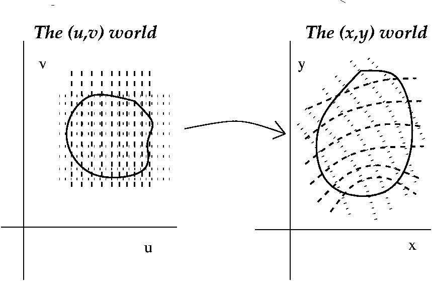 The idea of the last lecture was to replace an integral in (x,y) space
by an integral in (u,v) space which would be easier to
compute. Normally the u and v are geometric or physical quantities of
interest, and the "transformation" of the integral is suggested by
common features both of the domain and of the integrand. So the
integral over a region in (x,y) is thought of as a sum of f multiplied
by dA's. Then the dA's are each changed into (Jacobian) du
dv. That's what I tried to explain last time! The picture to
the right sort of shows what a decompostion into little dA's might
look like. Each dA is du dv multiplied by a distortion factor or
an area multiplication factor: the Jacobian. In general, the change of
variables formula for double integrals is something like this:
I think I will temporarily skip sections 15.6 and 16.6: I will deal with them later. I would like to try something maybe I can handle better(?): triple integrals. This is the content of section 15.7. Generally a triple integral is something which involves a function defined in a region of space, R3. Let's call the domain region a "blob". If we want a nice interpretation of what the triple integral computes, consider that the blob might be some sort of solid, and the function could give the density of the solid. At certain points in the blob, the function could be very small, corresponding to "lighter" parts of the solid. At some points, where f is very large, the blob is heavier. How could we determine the total mass of the solid? Well, in a real solid, the density probably doesn't vary very much from place to place. Therefore, in a small chunk dv of the solid, the total mass dm is probably approximately f(some sample point in the small chunk) multiplied by dv. This approximation will likely get better as the small chunk gets smaller. The total mass is the sum of all these little masses. Thus we are "led" to a quantity for the total mass which is a triple integral over the "blob". I would hope that a student in a math course would recognize that the formal underpinning of what's happening involves Riemann sums in 3-dimensions and limits. The first and simplest way to attempt to compute a triple integral is to convert it into a triply iterated integral. Example 1 was something like this (clearly very artificial!). The "blob" is the unit cube in R3 defined by 0=<x<=1 and 0=<y<=1 and 0=<z<=1. Suppose the density is x3+y2+z. What is the total mass (I omit any units here because I would probably get them wrong)? I claim that this is the same as
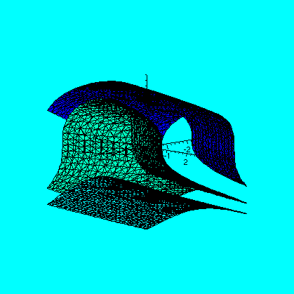
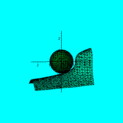
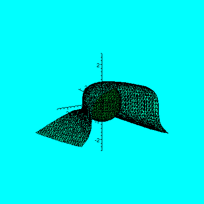
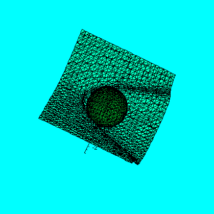
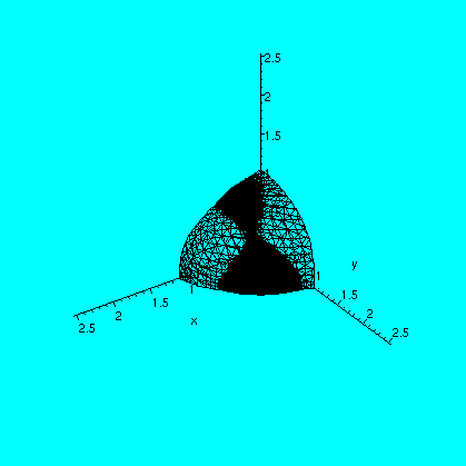
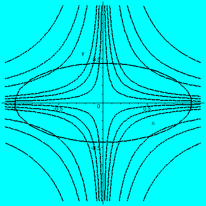
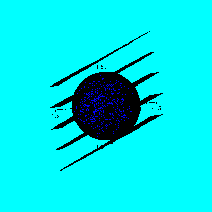
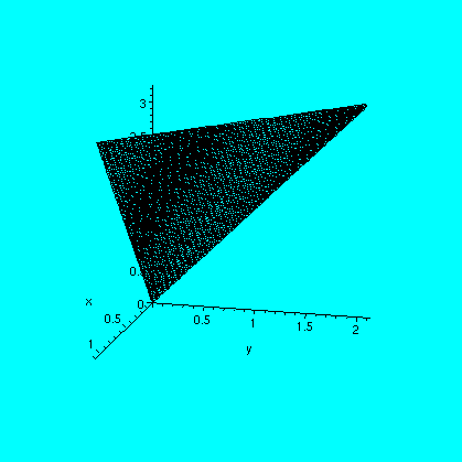
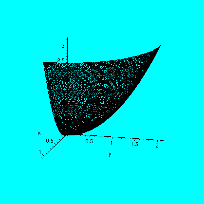
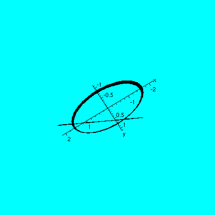
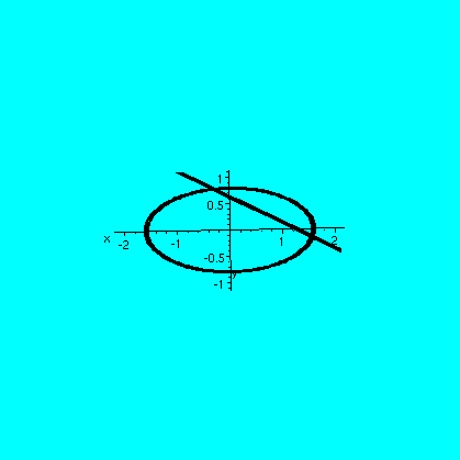
Example 3 I sketched and then gave out pictures of parts of a paraboloid and a plane, both going through (0,0,0) and (1,0,3) and (0,2,3). The first two pictures below are similar to the handout. I asked people to set up the limits on an iterated integral to describe the volume enclosed by these surfaces and the plane z=3. I divided the class into 6 groups, each with one of the iterated orders. This proved more difficult than I had anticipated. Part of the reason is that it was new. Part was also because the solid was not totally inside the "first octant", defined by x>0 and y>0 and z>0. It "oozed out" the edges. The third picture below shows why: it attempts to display a piece of a slice of the solid near z=2: it is a tilted view. The fourth picture shows this slice in an xy-plane. The straight line divides the ellipse into two regions, and the smaller part, the part which is mostly in the first quadrant, is inside the solid. The other part is outside the solid. The intersection points are needed (which will involve z, surely!) to get the limits on x and y. I thank David Jackson for pointing this out after class. The problem is difficult. Professor Ferry, instructor of a section of Math 251, has kindly posted Maple solutions to some problems of section 15.7.
| ||||||||||||||||||||||||||||||||||||||||||||||||||||||
| 10/30/2002 | We began by computing a very important integral:
int-infinityinfinity exp(-x2) dx. I first
sketched the curve y=e-x2 carefully. Then I
asserted that the "letter" defining the integral didn't matter:
I= int-infinityinfinity exp(-x2) dx =
int-infinityinfinity exp(-w2) dw =
int-infinityinfinity exp(-z2) dz etc. Therefore,
Now what we did last time can be used: both the integrand (x2+y2) and the region of integration (R2) are circularly symmetric. Therefore we rewrite the double integral as an iterated integral in polar coordinates: This integral is responsible for so many many many (no exaggeration!) occurrences of Pi in various formulas. Most importantly, it is involved in what is called the Central Limit Theorem. Google gives 134,000 results when asked to look for pages containing the Central Limit Theorem (CLT). Here is a simple Java applet which demonstrates the CLT through simulation of dice throwing. The CLT is probably the most famous result in probability. If you are interested in this subject, think about taking Math 477. You will have the prerequisites by the end of this course.
This challenge problem was designed to show off a certain technique, that of finding nearly hidden "symmetries" and then taking advantage of them. Here notice that the boundary lines are:
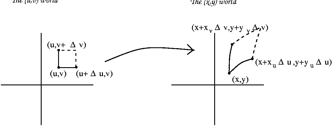 The computation resulted in the following: the (u,v) area of (delta)u*(delta)v was transformed into an approximate parellelogram of area |xuyv-xvyu| (delta)u*(delta)v. The bold-faced material can be thought of as an area magnification factor in going from (u,v) space to (x,y) space. It is officially called the Jacobian. I tried to do several "simple" examples to show that we had already seen such factors. One example was polar coordinates, where x=u*cos(v) and y=u*sin(v). The Jacobian turned out to be just u (this gives an algebraic explanation for the formula we developed last time, that dA=r dr d(theta): this is a very non-linear, non-uniform area multiplication factor. I also tried to find the area inside an ellipse. I think the specific ellipse was x2/4+y2/9=1. The transformation here was x=2u and y=3v. Then the ellipse came from the unit circle with area 1 in (u,v) space, while the Jacobian was 6: areas get multiplied uniformly by 6. SO the area of the ellipse was 6 times the area of the unit circle, so it was 6Pi. What's the general idea?
I returned to the challenge problem and computed the Jacobian, which turned out to be 1/4. The transformed integral (transformed into (u,v) terms) turned out to be int-11int01 u50v40 (1/2)du dv, which is easily enough computed to be (1/2)(1/51)(2/41).
The class was notable for the extraordinarily large number of errors of the lecturer. The patience of the students is very much appreciated. Mr. Huang kindly noted that the take-home surprise quiz needed to be corrected: the equation z=x2+y2 should read z=4-(x2+y2): yet another error! One "application" of change of variables is notable. I did not want to show it in class because it is ludicrous and almost fiendishly clever. I worry that a student who saw this would almost certainly never think that mathematics can be done by ordinary human beings. On the contrary, mathematics is done by human beings with limited intelligence but who are usually quite stubborn, or, perhaps, persistant is better. One infinite series whose sum is frequently quoted in introductory calculus is: | ||||||||||||||||||||||||||||||||||||||||||||||||||||||
| 10/28/2002 |
I began by considering the following problem: what is the volume
between the xy-plane and the graph z=4-(x2+y2)? I sketched this
volume. The "curvy surface" is actually just an inverted paraboloid,
whose cross-sections parallel to the xy-plane are circles. It has a
local and absolute max at (0,0,4). I can think of several methods to
compute this volume. First, one could compute it using 1-variable calc techniques. The volume described is the volume of a solid of revolution, revolved around the z-axis. The profile curve isn't very complicated. I didn't follow this up, but I hope people could do it. Another way is to use double integration. That is, compute the volume as the result of a double integral: int/int_{Base} Height dA, where the volume is just some Height over a region, the Base, in the xy-plane. Here one "intuitively" (after you think about it for a while!) realizes that dV, a piece of the volume, is Height*dA. In our case, the Height is given by z=4-(x2+y2). What about the Base? That's going to be gotten from intersecting the paraboloid with the xy-plae, or z=0. So x2+y2=4 results, and the base is the region in the plane inside a circle of radius 2 (the square root of 4) centered at (0,0). To compute the double integral, we change to an interated integral. In this case, either order gives the same amount of work. I think the class suggested dy dx. The x limits on the outer integral are fairly easy: x should go from -2 to 2. The y-limits, for a typical x-slice, are gotten by letting y go from the lower limit in terms of x to an upper limit in terms of x. Since the boundary of the base is given by x2+y2=4, we see that y=+/=sqrt(4-x2) and the iterated integral we need to compute is int_{-2}2 int_{-sqrt{1-x2}^{sqrt{1-x2} 4-(x2+y2) dx & nbsp; dy. I computed this. The inner integral is just a polynomial, and is easy to do. The next level, after some algebraic trauma, gives a constant multiplied by the integral of (4/3)(4-x2)^{3/2} dx from x=-2 to x=2. This can be done with a trig substitution: x=2 cos(theta). The resulting integral is int_{-Pi/2}^{Pi/2} (cos(theta)^4 d(theta). The x-limits become the theta limits. I then found an antiderivative using the double angle formula twice. Sigh. Any sane person would use Maple. I jsut did, and Maple got the same answer I did (8Pi) but maybe I should feel more virtuous because I did it without a machine. I don't.
Here the original volume when described as an iterated integral in polar coordinates is just int0^{2Pi} int02 (4r-r^3) dr d(theta). It is easy to compute, and just gave 8Pi again. As a simple exercise (hah!) I asked what plane parallel to the xy_plane would cut this volume in half? So we search for a value of H between 0 and 4 so that the volume above z=H under z=4-(x2+y2) was equal to 4Pi. After some pain (!) this came down to finding out what H made the double integral over the circle of radius sqrt(4-H) centered at 0, with integrand 4-(x2+y2)-H (the difference in the heights!) equal to 4Pi. This was most easily done as a polar integral: int02Pi int0sqrt(4-H) (4-r2) r dr d(theta) = 4Pi. After some computation, we got a quadratic for H, and it wasn't very complicated. The roots were 4+/-2*sqrt(2) (I just checked this with Maple and we were correct in class!). One root (4+2*sqrt(2)) was too large (bigger than 4!) so the other root is the only one to "keep". The only solution is 4-2*sqrt(2). I then tried to verify, as promised, that the earth is flat. Well, not verify, but try to see what the consequences of some simple assumptions are. We began with Newton's universal law of gravitation. This states that if m_1 and m_2 are two "point masses" which are a distance r apart, then the force of gravity between them has magnitude directly proportional to the product of the masses and inversely proportion to the distance between the masses. This means that there's a constant, usually called G, so that the magnitude of the force is G(m_1)(m_2)/r2. The direction of this force is attracting, and it runs from one point to the other. This "law" can be verified to very great accuracy by experiment.
Because 1) this is the polar coordinates lecture, and 2) the domain and the integrand both are circularly symmetric, it is probably a good idea to change to polar coordinates. Note that Gm(rho)d is all a constant for the integration, so it all "comes out". We are left with an integral over all of R2. But described in polar form this is int0^{2Pi} (for theta) and int0infinity (for r). The integrand is r dr d(theta)/(r2+d2)^{3/2}. This is wonderful since the darn "r" on top is exactly what is needed to get a nice antiderivative. The integral0infinity (r/(r2+d2)^{3/2}) dr is the limit of the integral from 0 to B as B--> infinity. An antiderivative of (r/(r2+d2)^{3/2}) is just -(r2+d2)^{-1/2}. Now evaluate this at B and subtract off its value at 0. The result is -(B2+d2)^{-1/2}-(-1/d) and as B-->infinity, the first term--> 0 and the result is that the improper integral is just 1/d. Going back to the whole original computation, the result is Gm(rho)d/d*(2Pi) (the 2Pi comes from integrating a constant from 0 to 2Pi) and the final answer is Gm(rho)(2Pi). This is really amazing because there is no d in the answer. the distance doesn't matter in this model. This is sort of "scale invariance". A person with great physical ?sense? could perhaps see this if one notices that, as you change d, the amount of plate inside a right circular cone with constant aperture increases, but it increases by a factor of the square of the distance while the influence of the distance itself is diminishing by the square: these balance out! Probably the earth is not flat, although its attraction to me doesn't seemingly diminish when I climb higher. Sigh. One physical situation where this is more or less physically correct is if one takes an electron, very very small, and a capacitor plate (from the electron's point of view, it might almost be infinite). So this analysis is approximately correct in that case. | ||||||||||||||||||||||||||||||||||||||||||||||||||||||
| 10/24/2002 | A surprise quiz was
given. I remarked that the double integral of x^3+y^3 over the
rectangle gotten by having both x and y between -1 and 1 was 0, and
Maple confirmed this. But also the integral of
sin(sin(x)+y^3) on that rectangle was 0: Maple could not
compute this integral. I knew it was 0 because the rectangle was
symmetric with respect to (0,0): both (x,y) and (-x,-y) were in the
rectangle. And the integrand, sin(sin(x)+y^3) was antisymmetric or
odd: its value at (-x,-y) was the negative of its value at (x,y). So
in the Riemann sums, there is cancellation of each piece with its
opposite through the origin. We reviewed the situation: double integrals, iterated integrals, and that they are equal (Fubini's Theorem). Of course I wanted to look at a peculiar function: f(x,y)=1 if x=y, and 0 otherwise. Does this f have a double integral over the "unit square" (x and y both between 0 and 1)? It is not continuous, so it definitely needs some special attention. I looked at the upper and lower sums if the intervals [0,1] were each divided into n equal parts. On "most" subrectangles, the max and min were both 0. But the diagonal subrectangles had places where f was both0 and 1. There were n of these rectangles, each having dimension (1/n) by (1/n). The discrepancy between the upper and lower sums was measure by the size of the sums on just these diagonal subrectangles (the ones which intersected y=x). But there were n of these subrectangles, and the max-min on each was 1, and the area of each subrectangle was 1/n2. So the difference was n(1/n2)=1/n. And as n-->infinity, this -->0. So one way of interpreting this is that 1-dimensional problems aren't "seen" by a 2-dimensional integral! Then we tried to compute a volume of a certain solid. The base was the triangle with vertices (0,0), (1,0), and (1,1), and the height over the point (x,y) was given by x2+y2. Some time was devoted to getting even a poor sketch (!) of it. Then I became ultra-pedantic. A pedant, according to my on-line dictionary, is:
How can one evaluate the double integral? We could try to convert it into iterated integrals. I think I first tried to look at the dx dy order. Here we could stop "adding" the little subrectangles when y=x: in fact, the iterated integral obtained was: int0^1 int0^y x2+y2 dx dy. I computed this integral: the inside was (4/3)y^3, and then integrated again from 0 to 1 the result was (1/3). The iterated integral in the other order was int01 intx1 dy dx. The inner integral now evaluates to x2-(4/3)x^3+(1/3). Integrating this again from 0 to 1 "dx", the result is 1/3. The two final results agree, but the intermediate stages are rather different, as are the upper and lower "limits" on each integral sign. This can be rather confusing! I concluded by finding a somewhat more complicated volume: the volume of a solid whose base is the region in the plane between y=x^3 and y=4x (curves intersecting at (0,0) and (2,8)), and whose height is given by z=3x+2y. This is more complicated. The volume is essentially the double integral over the base of the height function. So we decide to do it as the iterated integral int02 int_(y=x^3)^(y=4x) 3x+2y dx dy. According to Maple the inner integral is 28x2-3x^4-x^6. Then the outer integral is (3904/105). I emphasize that I am quoting Maple results done in another window: the irritations of this and the following computation when done by hand are not small! Integrating in the other order results in this iterated integral: int08 intx=y/8x=y^(1/3) 3x+2y dx & nbsp; dy. The algebraic description of the boundary curves here is quite simple, so it is "easy" to solve for x in terms of y. The inner integral here is (3/2)y^(2/3)-(19/32)y2+2y^(4/3): this is a mess, so it is probably better that I didn't do it in front of you. Then this integrated dy from 0 to 8 actually does (according to Maple) result in the same answer as above (thank goodness). This is what theory predicts. Please try some of these yourself. Practice is important in developing "intuition" and skill. | ||||||||||||||||||||||||||||||||||||||||||||||||||||||
| 10/23/2002 | We returned to the problem of fluid flow. For example, how
could one tell how much water went down a stream between 11 AM and
noon? One way might be to just dam the stream and collect all the
water during that period of time in a big reservoir with simple
"geometry" (a cylinder, for example). This could work. It might be
impractical, or even, in certain other similar situations, rather
difficult. So imagine someone wanted to know how much blood flows through my aorta during some specific
hour. I would rather not have this cut open and have all the blood
flowing though it collected ... also the procedure would likely
disturb the quantity being measured. So we should sample the blood flow. Insert a small "waterwheel", some paddles, etc. For example, we could measure something at 11:30, say, and learn that the blood flow is 3 cubic centimeters per min (cc/min). There are 60 minutes, so maybe the total flow is 60·3=180 cc's (Note What I know about physiology is close to nothing -- these numbers are totally invented!). Of course, blood flows varies with time. Maybe we would get more accurate estimates by increasing the number of samples. For example, we sample again at, say, 11:20 and get 2.5 cc/min, and at 11:40 and get 3.5 cc/min. From this information we might decide that blood flow during the first 20 minutes was "at" the first rate, then during the following 10 minutes at the 11:30 rate, and during the last half-hour at the 11:40 rate. Yes, the strategy here is not at all clear, but we would be led to some sort of sum of rate·time. O.k.: most students should recognize this setup. Here is the mathematical language. We start with an interval, [a,b], in R, the real numbers, and a function f defined on this interval. We partition th interval: a=x0<x1<x2< ...<xn=b into n distinct subintervals. The length of the jth subinterval is xj-xj-1. Inside each subinterval we select a sample point, called in many textbooks xj*. We then add up things: we take the sumj=1nf(xj*)(xj-xj-1. This is a rather complicated construction. This is called a Riemann sum, and depends on the selection of partition and sample points: lots of choices. Sometimes textbooks define special Riemann sums: the upper sum is gotten when the sample points are chosen so that the numbers f(xj*) are each the maximum of f in the specific subinterval. The lower sum is gotten when the sample points are chosen so that the function values are each the minimum of f in the specific subinterval. Any Riemann sum is "trapped" between upper and lower Riemann sums. I tried to illustrate this with pictures of areas of rectangles, but it is important to realize that although the initial motivations given to students for this whole set-up are computing areas, more realistically few area computations are needed in "real life": it is sums of things like fluid flow which should be kept in mind. Now how to get better and better approximations of the total "flow"? Certainly one needs to take more samples. In fact, just taking large numbers of samples may not guarantee a better approximation. Generally, one needs the samples to be distributed well though the interval, [a,b]. Again, in certain calculus books, the word "mesh" is used to describe the length of the longest subinterval of the partition. If the mesh-->0, then the number of sample points must get large (but not necessarily the other way around!), and we can hope that the Riemann sums will "approach" a limit. The limit is called the definite integral of f over the interval, [a,b]. We compute this quantity by using, say, the Fundamental Theorem of Calculus, if we happen to be lucky and know an antiderivative of f. In practice that's rare. Frequently numerical techniques must be used. Here is one way to estimate an integral: partition [a,b] into n equal parts, each of length (b-a)/n. Unfortunately, in practice one doesn't usually know how to select sample points for upper and lower sums, so getting a Riemann sum means that there is uncertainty about whether the result is an overestimate or an underestimate. But the Riemann sum will always be betwen the upper and lower sum. How much discrepancy can there be between the upper and lower sum? Well, look in the jth subinterval. What can the difference between f(at max)-f(at min)? According to the Mean value Theorem, f at max)-f(at min)=f'(in between)·(max place-min place). Now the difference (max place -min place) has got to be less than (b-a)/n, becasue these sample points are both in the jth subinterval, which has length (b-a)/n. And if we knew some estimate of the value of f', we could see that the total difference between the upper sum and the lower sum is (max of f' on [a,b])((b-a)/n)((b-a)/n)n. The n's are the important thing here. The first (b-a)/n comes from the use of the Mean Value Theorem. The second comes from the width of the subinterval. The last factor of n comes from the fact that there are n poissible subintervals, and the errors may reinforce each other. S the worst case possible is that the error can be no more than max of |f'| multiplies by (b-a)2/n. I actually did a specific example, something like sin(x^3+4x) in the interval [0,1]. Here f'(x)=cos(x^3+4x)(3x2+4), and the largest this can be is 7 (since sine's values are bounded by 1 and 3x2+4 is certainly less than 7 in [0,1]). b-a=1-0, so the error of a random Riemann sum with n equally-spaced partition points is at most 7/n. If we select n large enough, this certainly --> 0. I also discussed what might happen if we had a function with a discontinuity. Specifically, what if f(x)=1 for x>.5 and f(x)=0 otherwise. In this case, f is certainly not continuous and sure isn't differentiable. The previous reasoning doesn't apply. Such functions certainly arise in "real life" sharp shocks to physical systems, etc. If we want to see if this function can be integrated over the interval [0,1], then we partition the interval as before, etc. The difference between upper and lower sums is easy to analyze, especially if you draw a picture. The max and min in most subintervals are the same. The only disagreement is on one subinterval, around the jump in this f. The jump's height is 1, so the disagreement contributes 1 multiplied by 1/n, the width of the subinterval. As n-->infinity, this certainly goes to 0. So this function has a definite integral: a finite area "underneath" it. Now to look at the 2-dimensional situation. Here we'll have f defined on a rectangle R in the plane, R2. We partition each of the variables as in the 1-variable case: say n subintervals in the x direction and m subintervals in the y direction. We get a bunch of subrectangles (bunch here means mn subrectangles). In each subrectangle we select a sample point. Then evaluate f on the sample point, multiply the resulting number by the area of the subrectangle, and then (sigh!) take the sum of all these. The result is a 2-dimensional Riemann sum. It is true that if, say, f is continuous, as the "mesh" (the size of the largest subrectangle) -->0, then the Riemann sums --> a unique limit. This isn't really totally "clear" or obvious. The result is called the double integral of f over R. One interpretation of this, if f(x,y) is always positive, is that we have computed the volume of a solid whose base is the rectangle, R, and whose variable height at the point (x,y) is f(x,y). Computation of such an object can be irritating. The first approach that is tried is to use "iterated integrals". This corresponds to adding up the mn rectangles in different orders. For example, one can add up the sums in the row way first: integrating dx. The add up the columns: this is a dy integral. I tried a simple example (the details were too darn messy -- my example wasn't simple enough!). The example should have been something like the double integral of x2y over the rectangle defined by restricting x to be between 0 and 2 and y between 1 and 4. Then integrating dx from 0 to 2 gives us (1/3)x^3y)]x=0x=2=(8/3)y, and integrating that between 1 and 4 gives (4/3)y2]y=1y=4=(4/3)16-(4/3)1=60/3=20. The reverse order gives x2(1/2)y2]y=1y=4=(15/2)x2 and then (5/2)x^3)]x=0x=2=40/2=20. The results are the same. Note that the intermediate stages are rather different! | ||||||||||||||||||||||||||||||||||||||||||||||||||||||
| 10/21/2002 |
A general fact:
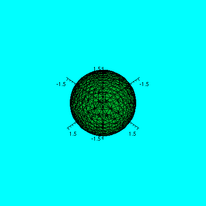
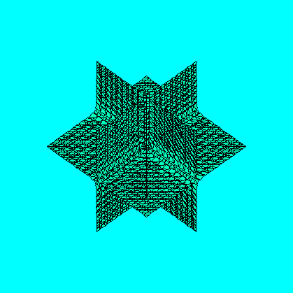
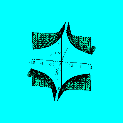
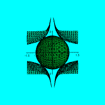
We analyzed two Lagrange multiplier examples. The process and analysis were described in a handout. Here are the pictures discussed in the handout. Further class material is described after the pictures. I strongly urge people who are interested to invoke their own copy of Maple and look at the pictures! My own choices of perspective and (ugh!) color will not likely be best for you. Also, you can rotate the pictures in Maple as you wish, and gain more insight. My experience tells me that "intuition" is obtained by working with examples. The labels (Fig.1, etc.) refer to those in the Lagrange multiplier discussion.
| ||||||||||||||||||||||||||||||||||||||||||||||||||||||
| 10/17/2002 | We studied the following problem:
consider the ellipse x2+5y2=1. Find the
rectangle of largest area inscribed in this ellipse with sides
parallel to the coordinate axes. Of course this turns into: maximize
4xy subject to x2+5y2=1. Consideration of the
geometry (varying rectangles) suggests that there is indeed a
"biggest" rectangle, somewhere. I suggested the following methods:
Here the constraint is x2+xy+y2=1, and the function to be maximized, the objective function, is x2+y2. The picture corresponding to this situation follows: 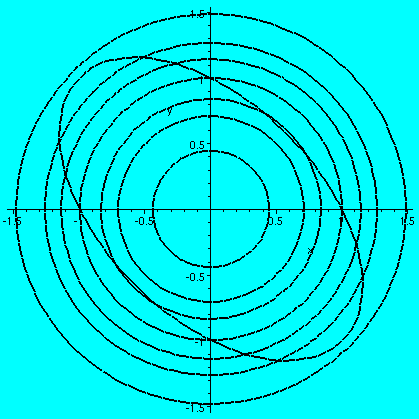
In fact, I asked if T(x,y)=x2+y2 were the temperature in a thin metal plate with shape the interior of x2+xy+y2=1, where will the plate be hottest or coldest? Well, local extrema only occur at critical points, and only (0,0) is a c.p. That, easily, is the coldest point in the plate. But where is the hottest point? It must be on the edge, and it will NOT be a local extremum, but only an extremum for a contrained maximization. We seek therefore the extrema on the boundary using Lagrange multipliers. Compute the gradients, etc. Then the multiplier equations and the constraint equation are: 2x+y=(lambda)(2x) 2y+x=(lambda)(2y) x2+xy+y2=1Again we can solve with (2x+y)/(2x)=(2y+x)/(2y) so x=+/-y (and possible special cases of x or y being 0). And so the temperature is going to be T(x,y)=2 or 2/3 since x2+xy+y2=1 gives x2=1 or x2=1/3. The solutions with x or y equal 0 yield T(x,y)=1. Here is a picture of these special isothermals, and the constraint. 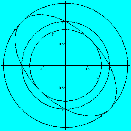
2x=3(lambda)
2y=-4(lambda)
2z=5(lambda)
x2+y2+z2=1
Here I chose to solve for x and y and z in terms of lambda, and substitute these values in the constraint equation, getting lambda=+/-(2/sqrt(50)). Then 3x-4y+5z turns out to be (for the two choices of lambda, generating two candidates for where extreme values take place) sqrt(50) and -sqrt(50). Here a final picture of the constraint and the two planes given by 3x-4y+5z=+/-sqrt(50). 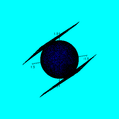
| ||||||||||||||||||||||||||||||||||||||||||||||||||||||
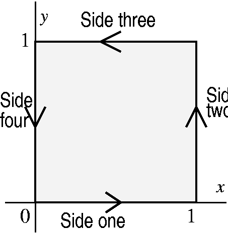 Now the most interesting thing is identifying what results as the line
integrals of the four boundary parts of the unit square. The first
integral, in red, is side two. Why? If we parameterize side two by x=1
so dx=0dt and y=t so dy=1dt with 0<t<=1, then P(x,y)dx+Q(x,y)dy
becomes P(1,t)0dt+Q(1,t)1dt=Q(1,t)dt, and the resulting line integral
is intt=0t=1Q(1,t)dt, which is the same as the
red integral (the letter used for the integration variable is a
logical place holder, and any letter may be used and will get the same
value). Similarly, the purple integral, the second one, is side four,
and the green integral is side three (the minus sign means the
integral is going "down") and the fourth integral, which is the blue
integral is side one.
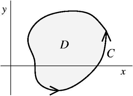
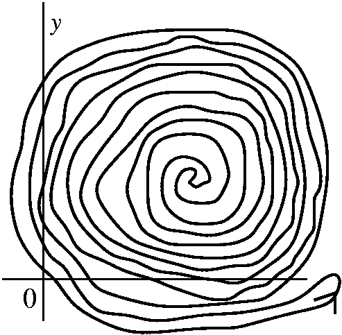 About the region and about the boundary curve The boundary curve
C should be a simple closed curve (there are some modifications which
can take care of this, to be mentioned later) which is oriented so
that the region D is on the inside of the boundary: that is, as you
travel around C, the region should be on the left.
This all seems very nice, and seems to fit the picture drawn last time
in our first statement of Green's Theorem.
However, the example displayed to the right should convince you that
sometimes it
may not be totally obvious what the "inside" of a curve is, or if a
point is on the inside, etc.. etc. What is shown is actually a simple
(non-intersecting) closed (start=end) curve. It isn't too easy to tell
if a random point not on the curve is inside or outside.
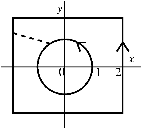 We returned to considering Pdx+Qdy where
P(x,y)=(-y)/(x2+y2) and
Q(x,y)=P(x,y)=(x)/(x2+y2), the example above. We
know that the work done around the unit circle is 2Pi. What is the
work done if we have a simple closed curve which does not enclose the
unit circle? Here we can apply Green's Theorem, and the answer is
0. But what if we have a curve which does enclose (0,0)? Let's try,
for example, the boundary of a square whose corners are (2,2) and
(2,-2) and (-2,2) and (-2,-2), as shown. What is the line integral of
our Pdx+Qdy over that square? Look at the dash line. Suppose we create
a closed curve which goes backwards around the circle, across the
dashed line, around the square, and the back on the dashed line. It is
the boundary of a region inside which the hypotheses of Green's
Theorem are fulfilled. There Py=Qx so the total
integral is 0. But the dashed line integrals, back and forth, cancel
out, and therefore the integral over the circle equals the
integral over the square. Both are 2Pi. In fact, here is how to detect
if any simple closed curve not going through (0,0) does or does not
enclose (0,0): compute the work of Pdx+Qdy around this curve. It is
either 0 (not enclosing the origin) or 2Pi (enclosing the origin,
usual orientation) or -2Pi (enclosing the origin, reverse of the usual
orientation). Notice also that Pi+Qj is not conservative
in any region enclosing the origin and has no potential in any such
region. But, almost paradoxically, in a region which doesn't enclose
(0,0), it is conservative, and does have a potential.
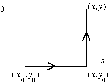 The secret is to use speical paths to verify these equalities. For
example, let's choose a path made up of two straight line segments,
one from (x0,y0) to (x,y0) and then
to (x,y). Call the first piece C1 and the second,
C2. So f(x,y) equals the integral of Pdx+Qdy over the path
C1+ C2. I'd like to compute the partial
derivative of f with respect to y. For this I will study how f(x,y)
varies when y varies. But there is no change in the C1 part
at all (since it goes from (x0,y0) to
(x,y0): there's no y varying there!). I just need to
study how the integral over C2 behaves. We parameterize
this integral: x=x (x does not change!) and y=t where
y0=<t<=y (yes, there are too many y's in all this
discussion!). Then dx=0 (remember, x does not vary) and dy=dt. So the
integral over C2 becomes the definite integral
inty0y Q(x,t) dt. I want the
derivative of this with respect to y, and this is exactlyu laid out so
that the Fundamental Theorem of Calculus applies. The answer is Q(x,y)
and we have verified that fy(x,y)=Q(x,y). To check the
other partial derivative, use a path made up first of a vertical and
then a horizontal line segment.
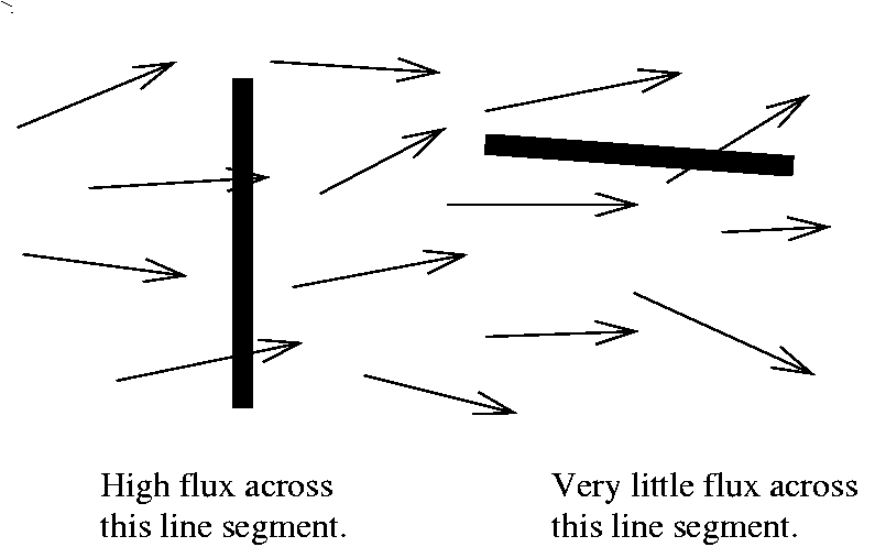 A somewhat analogous computation is important for the fluid flow
interpretation of vector fields. Here if we think of F as the
velocity vector field of a fluid, and C is a curve in the plane, we
might be interested in the net flow of F across C: this is
called the flux. In this case, the net flow is larger if the
curve is perpendicular to the vector field, and small if the curve is
almost parallel to the vector field. So the unit tangent vector is
replaced by the unit normal vector. Note that if
t=Ai+Bj
then n=-Bi+Aj, so the unit normal also has the
darn square root in the "bottom" to cancel the horrible (?) square
root coming from the computation of ds.
We will do much more computation and investigation of these line
integrals next time, including how to compute them efficiently.
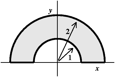 About the only thing I did that wasn't a homework problem was the
following, which I asked students to try (quoted from another calculus
text): suppose you have a mass distribution whose density is "Fred" in
the region
shown: here the boundary curves are semicircles centered at the origin
together with two line segments. Then the total mass will be the
double integral of Fred over the region. The task I asked students to
try was the following: describe how to compute this using dx dy
iterated integrals, and how to compute this using dy dx
iterated integrals. Here one must not assume either that Fred
is defined outside of the region indicated (so you can't integrate
over the "big" semicircle and then subtract off the part in the
"small" semicircle. Nor can one assume that the mass distribution has
any symmetry (why should Fred be the same on the right and left side
of the y-axis, for example?). Each order apparently takes 3 standard
iterated integrals to describe. In polar coordinates, of course, this
is just one integral.
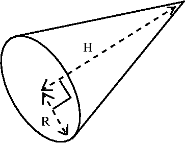 A right circular cone with height H and base radius R is shown to the
right. The "right" in the description refers to the fact that the axis
of symmetry is perpendicular to the base. The "circular" means that if
the cone is cut by a plane perpendicular to the axis, then the slice
will be a circle. The axis of symmetry is the line from the corner or
vertex of the cone to the center of the circular base. The picture
shown is an oblique one, so the base appears elliptical.
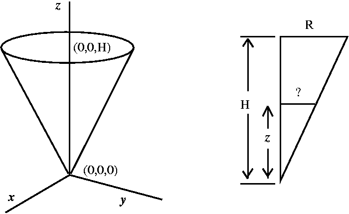 Then how can we compute the moment of inertia. I was advised to call
the moment of inertia of a small piece dI, so the total moment of
inertia was the triple integral over the whole cone of dI. We compute
the total moment of inertia using a conversion to an iterated
integral. I did this dx dy dz, ignoring various moans from
the audience about some silly thing called "polar coordinates". The
limits dz were from z=0 to z=H. Then a "typical" constant z-slice was
a circle in the xy-plane. The radius of that circle was shown to be
given by (R/H)z. So the boundary of the circle was
x2+y2=(R2/H2)z2.
And the limits of the integral were:
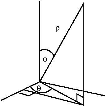 For spherical coordinates, rho is the distance from (0.0.0) to
(x,y,z). Theta is the angle from the positive x-axis to the bottom
of a line segment from the point "dropped" perpendicularly to the
xy-plane. Phi is the angle from the positive z-axis to the line
segment from the origin to the point. Finally, rho is the distance
from (0,0,0) to the point. I wrote various complicated formulas for
conversion from rectangular to spherical coordinates. I emphasized
that I hardly ever recalled these, but I did remark that it was useful
to remmber that rho2 was the same as
x2+y2+z2. Everybody should see the
formulas, and know how to use them if they had to. I also sketched the
points where phi=Pi/6 (a cone, vertex (0,0,0), central axis the
postivie z-axis, and "aperture" given by Pi/6 from the z-axis). It is
conventional that phi be restricted to lie between 0 and Pi. I
sketched what theta=Pi/6 was: a half plane, with the z-axis in its
boundary, at an angle of Pi/6 fromt he positive z-axis. Here it is
conventional for theta to be between 0 and 2Pi. I also remarked that
it is conventional in all this for rho to be non-negative. And, of
course, the collection of points with rho=3 is a sphere of radius 3,
centered at the origin.
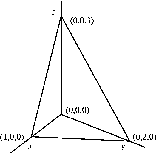 Example 2 involved a tetrahedron, which is a solid in
R3 with flat sides and 4 corners. Suppose the corners are
(0,0,0) and (1,0,0) and (0,2,0) and (0,0,3), and again the mass
distribution is x3+y2+z. Can we set up a triple
iterated integral to compute the mass? I asked for some suggestions
for the order. I mentioned that it was not clear to me that the order
actually mattered very much here for ease of computation. So we tried
dx dy dz first.
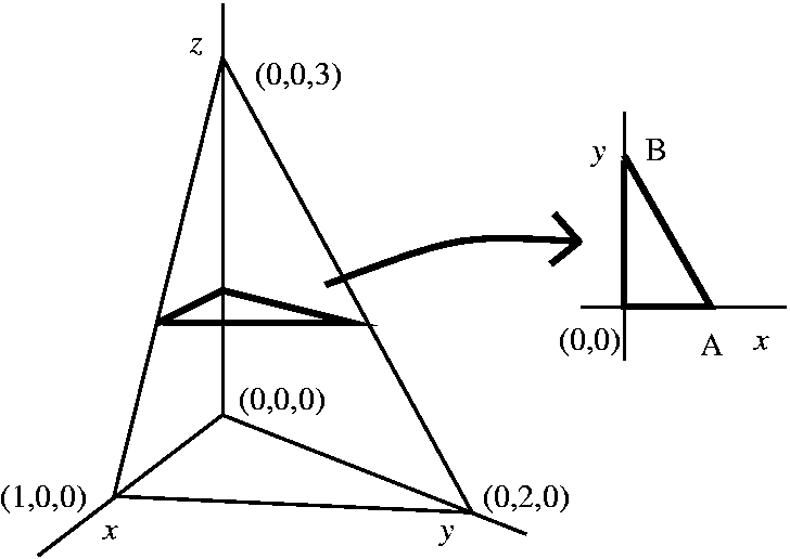 I try to do the integrals from the "outside" to the "inside", doing
the outside-most integral first. "Clearly" the dz integral will have an
upper and lower limit. These limits correspond to the top and the
bottom of the solid. The bottom is z=0. The top is z=3. What about the
inside, which is dx dy? We need to see what a "typical" slice
when z="constant" looks like in order to get the dx and dy limits. A
pciture shows that the slice is a right triangle with edges along the
x and y-axes. But what are the coordinates of the points A and B
shown? The line segment is part of the "tilted" face of the
tetrahedron. That face is part of the graph of a plane: Px+Qy+Rz=S for
some constants P and Q and R and S. We can guess the constants or we
can just write vectors along various edges of the tetrahedron, take
cross-products, etc. Well, the plane is x+(1/2)y+(1/3)z=1. So the line
in the xy-plane is x+(1/2)y=1-(1/3)z. Remember in this slice z is
supposed to be constant! Then we can get the coordinates of A by
taking y=0 and the coordinates of B by taking x=0. So A must be
(1-(1/3)z,0) and B must be (0,2-(2/3)z). The lower limit on the dy
integral is 0 and the upper limit, the biggest y can be in this slice,
is 2-(2/3)z. What about, finally, the x limits? Here we take a line
segment across the triangle, in a horizontal direction. The smallest x
value is x=0, and the largest x-value is given by whatever x-value
lies on the line. But the line has equation x+(1/2)y+(1/3)z=1, so x
must be 1-(1/2)y-(1/3)z. The triple integral limits for the
tetrahedron in this order are:
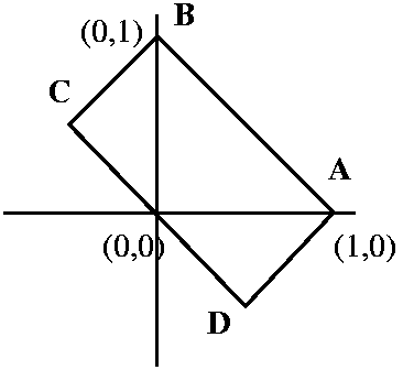 My challenge problem of the lecture was the double integral of
(x+y)50(x-y)40 over the rectangle R shown.
Although the function involved is a polynomial, and therefore in some
sense nearly trivial to antidifferentiate, and the region is a very
simple rectangle, in fact computing the actual value of the integral
is not easy. A straightforward transition to either a dx dy or a
dy dx integral is equally irritating. Actual computation means
finding equations for the boundary lines, and breaking up into three
different iterated integrals. Then antidifferentiating, which, while
simple in "theory", in practice would be irritating.
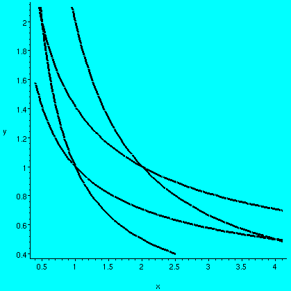 I concluded by doing problem #16 of section 15.9. Such curves and
integrals arise in the theory of adiabatic processes ("one with no
heat transfer in or out of the system"). The Adiabatic Gas Law
for an ideal gas which is thermally insulated is PVa
constant= another constant. Then the closed boundary curve in
this problem is
related to something called a Carnot cycle. I wanted to remark
that the problem wasn't quite a weird as it looked. So I graphed the
region given, and to the right is a Maple version with this
instruction (notice that the picture is uncontrained, so the x
and y axes have different units):
implicitplot({x*y=1,x*y=2,x*y^2=1,x*y^2=2},x=.4..4.1,y=.4..2.1,
thickness=3,grid=[30,30],color=black);
I worked through the steps outlined above, and magically (!)
all the details made sense. If u=xy and v=xy2, as suggested
in the text (thus doing step 1 above for us) we were able to write x
and y in terms of u and v: y=v/u and x=u2/v (this is step
2). Then the region is 1=<u<=2 and 1=<v<=2 (step 3) while
the integrand is y2 which turns out to be
v2/u2. The hardest detail in all this stuff is
usually computing and "understanding" the Jacobian. The computation is
straightforward here, and the Jacobian is 1/v. The integral is then
fairly easy: int12 int12
v/u2 du dv whose value is 3/2, I think.
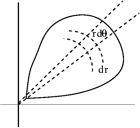 I maintain that neither of these methods are the way a sane and
informed human being would do the problem. Both the Height and the
Base have lots of circular symmetry, and the problem is more naturally
done taking advantage of this symmetry: Use polar
coordinates!. Here i mean x=r cos(theta) and y=r
sin(theta). More importantly (and how I usually recognize
symmetry) is the presence of x2+y2 in the integrand and in the
defining equation for the boundary of the base. I remarked that a
double integral over a region was transformed into an iterated
integral by adding up the boxes in first horizontal then vertical
order (for dx dy) and in the other order for dy dx. The dA
was changed to dx dy or to dy dx. For polar decomposition,
though, I need to break up the region using rays out from the origin
with angle between them of d(theta) and circular arcs with distance
between them of dr. But if you look carefully, you'll see that the
length on the theta part is amplified by the distance from the
origin. In fact, dA is actually most accurately represented by r
dr d(theta). So the integral is int int (4-r2) r dr
d(theta). Nere the limits on the integral need to be described
in polar coordinates. Certainly theta goes totally around the circle,
from 0 to 2Pi. More interestingly, r goes from 0 to 2, from the center
out to a circle of radius 2.
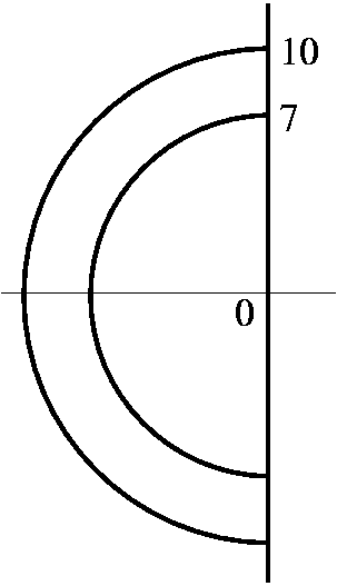
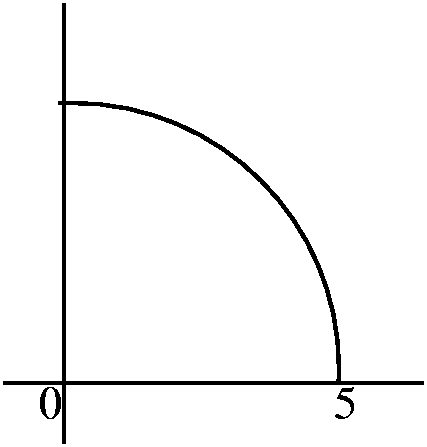 As an exercise, I asked people to "describe" for integration purposes
two regions. The one on the left was described by theta between 0 and
Pi/2. The one on the right was supposed to be a piece of an annular
region, and theta was between Pi/2 and 3Pi/2 and r, between 7 and 10.
It certainly is possible to describe the unit square in polar
coordinates (!!) but it is likely to be an unnatural exercise, so why
bother?
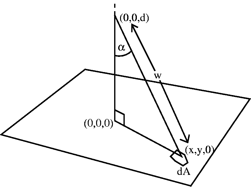 What is the gravitational attraction of a homogeneous doubly infinite
thin plate to an external point mass? Here I mean that the point mass
has mass m, and that the thin plate has mass density rho, so that a
chunk of the thin plate with area dA has mass rho(dA). How should we
compute this attraction? We set up things so that the external mass
was at the point (0,0,d), and the thin plate was the xy-plane. Then
the force of attraction has magnitude (m(rho)dA)/w2, where w is the
distance from (0,0,d) to (x,y,0). This is sqrt(x2+y2+d2), so
w2=x2+y2+d2 (slightly simpler!). But this is the force. Note that
the piece of plate at (x,y) "balances" the piece of plate at
(-x,-y). By that I mean that the total of the forces from the two
pieces has 0 horizontal component- the i and j parts are opposite. We
just need to figure out the k component. To get the magnitude of the k
component we should multiply the magnitude of the force by cosine of
alpha, where alpha is as shown: that gives the correct "correction"
(nothing like redundancy!) for the k component. Now, wonderfully, the
cosine of alpha is d/w=d/sqrt(x2+y2+d2). So this gives as integrand
Gm(rho)d(dA)/(x2+y2+d2)^{3/2}. And this is to be integrated over all
of R2.