Cryptanalysis of the NFL Schedule

Stephen D. Miller

Rutgers University

January 12, 2016

This is a companion piece to my interview with John Urschel in the February 2016 Notices of the American Mathematical Society.  It aims to explain in everyday terms how some principles of codebreaking (or “cryptanalysis” as it is called by those in the community) can be applied to see a bias in a familiar scheme: the NFL schedule.  We’ll see that in certain years (including 2015), the NFL schedule has an unexpected quirk that might explain why the New England Patriots and Carolina Panthers had such strong seasons.  I’ll also explain how to use mathematics to fix the problem, and touch upon some exciting current mathematical topics such as the “Graph Isomorphism Problem”.

Codebreakers often find themselves face-to-face with a complicated, impenetrable-looking cryptosystem that seems to offer no hint as to how to attack it.  Usually they fail, but occasionally careful scrutiny will reveal a small design flaw that causes a pattern to repeat itself more often than it probably should.  Alternatively, there might be an unintended, very small lack of randomness that biases the encryption a particular way.  Once that small crack in the ice is taken advantage of, a fortunate attacker can sometimes leverage it to defeat the entire cryptosystem.  A classic example is the “Cryptogram” found in newspaper comics sections, in which each letter of the alphabet is encoded as a different letter (these are also known as substitution ciphers). The English language uses letters like “e” and “i” more frequently than “j” and “x”, and this bias makes it possible to crack such codes even as a recreational hobby.

I’ll explain a toy example of the cryptanalysis methodology applied to the NFL schedule.  Of course the NFL schedule is not cryptic: everyone knows what it is in advance, and so the allusion to cryptography is merely an analogy.  We will see that in certain years ­-- including 2015 -- the schedule has very different features.  (For a peek, see Figures 1 and 6 below.)

The NFL Schedule rotation:  The 32 NFL teams are organized into two conferences (AFC and NFC), each of which has 4 divisions of 4 teams apiece.  Each team plays 16 games a season.  14 of those games are against rivals that are determined far in advance by a schedule rotation.  (It is this rotation which has the flaw I alluded to above.)  Here’s a schematic indicating who those 14 games are against:

Every team in a given division has a common list of opponents in 14 games.  They play every other team their own division, every team in another division in the conference, and every team in another division in the other conference.  The key point is that a team plays only 2 other games (marked in blue) aside from these set divisional matchups.  Those 2 games, which are played against other conference rivals, are against teams which finished the previous season in the same place in the standings.  Thus a team that finishes in 3^rd place in its division will play all other 3^rd place finishers in its conference the following year (one of these is already included in the green grouping). 

What’s the problem?  In setting up the rotation (which you can find neatly described here), the NFL was not careful about setting up the 4-year cycle of divisions from the other conference (marked in red).  They also apparently failed to take into account different possibilities which would have worked better (I’ll suggest improvements below, e.g., in Figure 3).  It could be there was an excellent reason behind this, but nobody I’ve spoken to is aware of one.  I am also unaware of any other league where the schedule structure varies so drastically in different years.  This causes an unexpected and unintended pattern which I’ll now describe.

As we just saw, 14 out of 16 of the opponents a team plays are determined by the schedule rotation, which is purely dependent on their division.  Here’s a schematic indicating the divisions that play each other in the 2015 season:

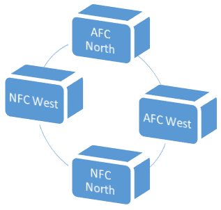
Figure 1: The North-West and South-East clusters in the 2015 NFL schedule.

Here I’ve connected two divisions with an arc if they play each other.  There is a very striking, unexpected feature here: there are 2 different clusters in this picture.  This means that, aside from the 2 games in blue against teams that finished equally ranked in the 2014 standings, there are no games between teams on the left and teams on the right.  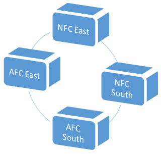In particular, 87.5% of all games are internal to these separate clusters: in 2015 teams in the East and South play very few games against teams in the North and East, which is not at all the case for 2016 when the schematic will look like this:

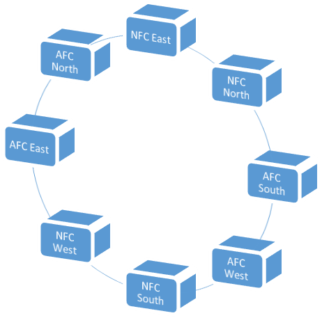
Figure 2: The 2016 schedule has just 1 cluster (unlike 2015's).

This 2016 diagram doesn’t isolate divisions into separate clusters.  In fact, in the full 12 year cycle, only 2 years (2012 and 2015, for example) have two disconnected clusters, whereas the other 10 years have diagrams like 2016’s which form one big circle (see Figure 3).

Put differently, it is well-known that AFC and NFC teams do not play each other often: only 64 of the 256 games each year are interconference games.  However, if we reorganize the NFL into the two different 16-team clusters in each of the two circles (i.e., the 16 teams which are in the South and East divisions of either conference, and the 16 teams which are in the North and West divisions of either conference), there is a staggeringly-low total of only 32 games played between them!  Thus in 2015 the NFL is arranged into geographic regions more than it is into conferences.

Can it be fixed?  Yes, though of course any changes would mean temporarily interrupting the current schedule rotation.  There are many ways to do it, all of which are mathematically similar.  Here’s a particular solution which involves only a slight modification of the current rotation:

Figure 3: My proposed schedule rotation, which eliminates the possibility of clusters that appear in the 2015 schedule (as in Figure 1).

The rotation repeats every 12 years, i.e., 2029 is like 2017, 2030 is like 2018, etc..  I’ve kept the previous coloring scheme with green referring to divisional pairings within a conference, and red for those with the other conference.  The changes here are minimal: the green part (within the conference) was not changed at all, and the only changes in matchups between different conferences involve a few switches involving the NFC North and South.

If this switch is adopted, then (due to the transition) teams in the AFC South would play NFC North teams in 2019, only 3 years after playing them in 2016 (see Figure 2); they would not play NFC South teams until 2020, 5 years after having played them in 2015.  This a slight deviation from the usual 4 year cycle, but only a temporary one: the 4 year cycle would resume again after this.  Aside from similar changes for AFC West teams against the NFC North and South, this is the only change I am suggesting.  However, it’s adequate to completely eliminate the clustering present in the 2015 schedule (Figure 1).

A Sudoku-style method of finding a schedule without clusters.  Having just given a schedule fix, let’s now see a fun way to understand why it’s possible to find one.  We’ll convert the problem into one similar to filling out a Sudoku grid.  In order to be flexible and not identify any particular divisions, let’s number the divisions AFC 1, AFC 2, AFC 3, AFC 4, and NFC 1, NFC 2, NFC 3, NFC 4.  For the sake of argument, let’s start this new system in 2017.  The following charts show

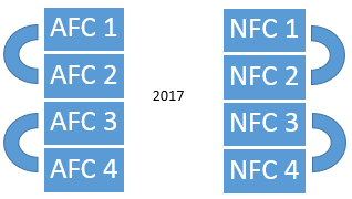
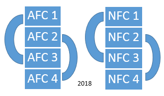
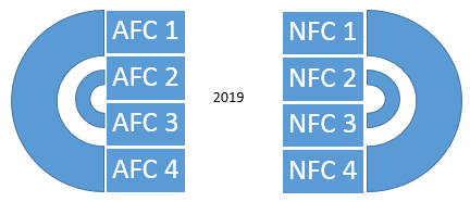
Figure 4: The proposal for matchups between divisions in each conference

the matchups between different divisions in the same conference.  The pattern repeats every 3 years, so that 2020 has the same diagram as 2017, etc..  Since I have not specified which divisions are which, these diagrams in fact account for all possibilities.  (The NFL actually uses such a scheme at present, though this is not important; it’s more convenient to assign the divisions numbers than names in this explanation.) 

We now turn to the 4-year rotation of divisions in different conferences, which I’ll explain using a 4x4 grid

that I’ll have to fill in with numbers 1,2,3,4 to tell you which NFC divisions the AFC divisions will play.  I need to make sure that each column uses the numbers 1,2,3,4 exactly once apiece (otherwise, two AFC divisions plays the same NFC division, while some NFC division plays no AFC division).  Also, the NFL requires all divisions to play each other within a 4 year cycle; this means that each row uses the numbers 1,2,3,4 exactly once apiece. 

Filling out the grid is now like filling out a Sudoku puzzle.  However, I am going to add a further stipulation that is not covered by the previous paragraph: I’ll insist the AFC 1 plays NFC 1 in year 1, AFC 2 plays NFC 2 in year 2, etc.:

This will be the key to explaining why the eventual solution does not produce clusters in the schedule rotation.  For now, note that because each number will occur exactly once in each row, it will never happen that (aside from these diagonal entries I just marked) AFC division 1 plays NFC division 1, AFC division 2 plays NFC division 2, AFC division 3 plays NFC division 3, or AFC division 4 plays NFC division 4.

Our task is to fill in the blank spots with numbers 1,2,3, or 4, so that each row contains each number exactly once, and each column contains each number exactly once.  To do this, let’s look at the bottom entry in the 2019 column (which I’ve highlighted in the following grid).  It can’t be a 3, since there’s already a 3 in that column.  It can’t be a 4, since there’s already a 4 in that row.  It must be a 1 or a 2 -- either will work, so let’s make it a 1:

Let’s now consider the second entry in the 2019 column, which cannot be a 2 (since there’s already a 2 in row 2), nor a 1 or a 3 (which are already in the column).  It therefore must be 4, which in turn forces the first entry in the column to be 2 (the only unused number):

The first entry in the 2^nd row must be 3 (since 1 is already in its column, while 2 & 4 are already in its row).  Therefore, the last entry in that row must be 1:

Now most of this grid is filled out.  The other entries are easy to deduce in a similar fashion, and the final answer is as follows:

We will use this grid not just for years 1,2,3, and 4, but furthermore extend it in perpetuity by repeating it every 4 years.  Incidentally, had we used the initial choice of 2 (instead of 1) when we started filling out the bottom entry of the 2019 column, we would have instead obtained the transpose of this grid (meaning what you get if you reflect it by a mirror on its diagonal).  These are the only two solutions.

Why does this remove clusters?  The grid is set up so that in a given year, there is precisely one number between 1 and 4, call it n, for which AFC division n plays NFC division n.  Because the AFC and NFC sides of each diagram in Figure 4 are identical, there is a different number, m, such that AFC division n plays AFC division m, and NFC division n plays NFC division m.  (That is, the division they play in their own conference has a common number.)  We constructed the grid so that AFC division m does not play NFC division m.  This means that whatever cluster AFC and NFC divisions n and m are in, there must be at least two other divisions involved, and so this cluster must have at least 6 of the 8 NFL divisions in it.  Could there be a division that’s not in this cluster?  Such a division must play 2 other divisions (one in its conference, one in the other conference), and so it would be part of another cluster having at least 3 divisions.  That would leave us with both our first cluster of at least 6 divisions, and this second one of at least 3 divisions -- none of which overlap.  That makes for at least 9 divisions, whereas the NFL has only 8 divisions.  We conclude from this contradiction that there can only be one cluster of teams (so that the diagram looks like Figure 2, though with different divisions labeling the boxes)

Some extra math – spectral graph theory: The way I noticed the 2015 NFL schedule quirk was in making an illustration for my interview with John Urschel in the February 2016 Notices of the AMS.  This picture

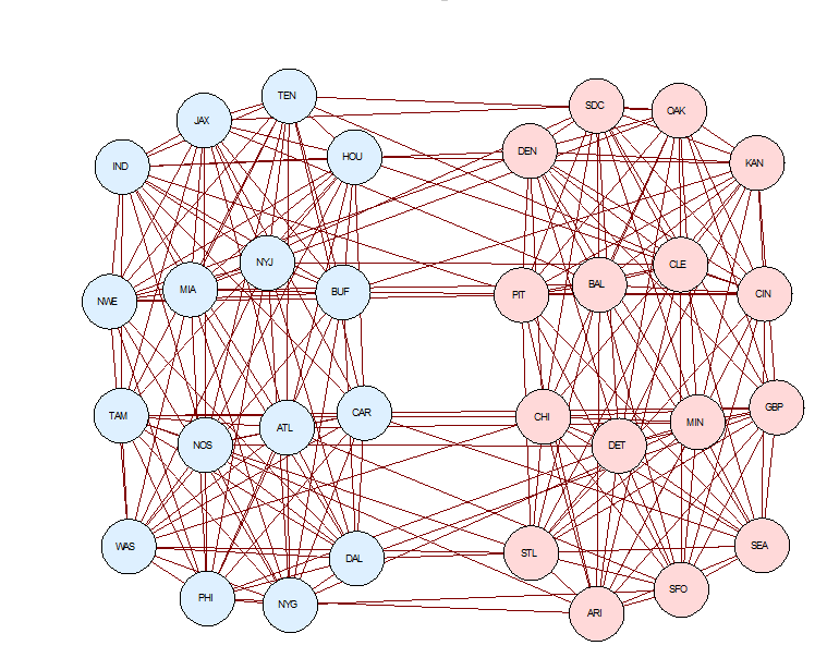
Figure 5: Graph from Notices article illustrating the Urschel-Zikatanov Theorem.

represents each of the 32 teams by a circle, and connects them by lines if the teams play each other in 2015.  Here’s how it looks in other years, with the circles shrunk to dots:

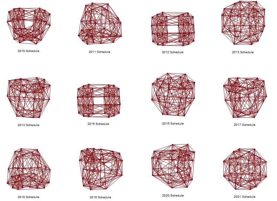
Figure 6: Schematic of the NFL schedule graphs from 2010-2021.  The diagrams repeat every 12 years, e.g., the picture for 2022 is identical to that for 2010.

Mathematicians call a network of lines connecting dots such as this a graph. The coloring in Figure 4 is in terms of the lowest nontrivial Laplace eigenfunction for the graph (see the sidebar in the article for more technical information).  It naturally selects clusters with few edges between them; in this case, it found the South-East and North-West clusters described above.  “Spectral partitioning of graphs”, as this is called, is a fundamental tool in analyzing data sets.  It finds patterns that might not be readily seen from other points of view (for more information, click here).

Figure 5 has 12 different looking pictures, but actually not all of them are really different mathematically.  For example, it’s not difficult to see that the 2012 and 2015 entries are extremely similar to each other: it is possible to reposition the dots (dragging their attached lines with them) to make them look exactly like each other.  In mathematical parlance, these graphs are called “isomorphic”, meaning they have the exact same shape (they only appear different if the dots are put on paper in different places).

What’s less obvious is that the other 10 diagrams are isomorphic to each other (but not to the 2012 or 2015 diagrams).  The task of determining whether or not two graphs are isomorphic is the famous “graph isomorphism problem” in theoretical computer science.  It can always be solved by brute force, but there are clever ways to vastly speed it up.  Recently Laszlo Babai of the University of Chicago announced an important breakthrough on this problem.

Another important mathematical feature is mixing time, which roughly speaking measures how long one has to walk around randomly along the lines between the dots before they’ve lost any trace of where they started.  Imagine that an army of ants emerges from a particular dot, and starts diffusing by walking along the lines connecting the dots to each other, making random decisions as to where to go next.  In the 2015 graph in Figure 5, the odds are not good that many ants will quickly make it across the relatively small number of lines bridging the two sides of the diagram, meaning that the mixing time is high.  However, in the 2016 graph the ants would diffuse faster.  This is measured by a statistic called the lowest graph eigenvalue, which is usually 6 for the graphs in Figure 6, but dropped to 4 in 2012 and 2015.  The higher this statistic, the more random looking the graph is. 

A mathematically related concept is that the 2012 and 2015 diagrams are easier to disconnect into 2 pieces (by cutting a small number of lines) than the other diagrams.  This is why New England and Carolina were shielded from having to play so many strong teams on the righthand side of the picture in Figure 5, and why the South-East cluster as whole had a higher winning percentage than it would have had if it had more exposure to the strong teams in the North and West.  The relationship between mixing time, eigenvalues, and disconnection appears prominently in the related mathematical subject of expander graphs.

Finally, let’s conclude with cryptanalysis.  Low mixing time is desirable in a cryptosystem, because it generally means an attacker has less information about the state of a system.  In terms of the ants, the faster they can spread around, the less information we have about where they first emerged from.  This is an important design feature in making stream ciphers (which are fast, secure random generators), and spectral graph theory is an important tool in analyzing cryptographic constructions because of its ability to find hidden patterns. 

Thanks: to John Urschel, Peter Sarnak, Keith Frankston, Michael Fruchter, and Nathan Keller for their helpful comments. 

Stephen D. Miller is professor and vice-chair of Mathematics at Rutgers University.  He can be reached at miller@math.rutgers.edu.  His research focuses on number theory (including the underlying mathematics of cryptography) and is supported by National Science Foundation grant CNS-1526333.