Here is a rather sophisticated example: {(50)n/n!}. The top is
bigger and bigger powers of 50, while the bottom is n!. Both the top
and the bottom grow. Understanding the asymptotic behavior of this
sequence as n→∞ is asked to
decide which grows faster, the top or the bottom. I mentioned in class
that this bizarre looking sequence is not random, and really does
occur in applications. Here is some numerical evidence (the first 7
terms, rounded to 10 digit accuracy):
50, 1250, 20833.33333, 260416.6667, 2604166.667,
2.170138889·107, 1.550099206·108.
If you want more evidence, than the 20th is about
4·1015, and that's quite big to me. But, in fact,
this sequence converges. It is important not to be deceived by
what happens for small n's. We are interested in
the asymptotics as n grows really, really big.
Some students noticed something like the following argument. Take n
to be an integer larger than 100. (You will soon see why I selected
100: it is because it makes some computations and comparisons
easier). Then
/ (50)n \     (50)(50)(50) ··· (50)
| ----- | =  ----------------------
\   n!  /      1·2·3·4·5···(n–1)n
Look at the product of the first 100 fractions above. This is some
enormous number (the top is (50)100 and the bottom
is 100! The valueof a100 is about 8·1011 actually. How
many terms are left over? The terms from 101 up to n, and that's n–100
(n minus 100) terms. Each of them has 50 on top, and a number bigger
than 100 on the bottom. So the leftover terms all are less than
1/2. That means:
{(50)n/n!}<
{(50)100/100!}(1/2)n–100.
The powers of 1/2 drive down the sequence values when n is
bigger than 100. I chose 100 because it would be nice to get some
definite number like 1/2, so you can see things decreasing. In fact,
when n=200, the value of the sequence element is about
7.89·10–36, quite small. I claim that the following
result is correct, but is definitely not "clear":
limn→∞{(50)n/n!}=0.
| Wednesday, November
4 | (Lecture
#17) |
|---|
Again, here is a version of what's called Taylor's Theorem:
If
Tn(x)=∑j=0n[f(j)(a)/j!](x–a)j,
then the difference between this and f(x) is
[f(n+1)(c)/(n+1)!](x–a)n+1 for some c between a
and x.
This difference is called the error or the remainder. I
tried to give several "simple" applications of Taylor's Theorem, doing
as much of the computatin as I could "by hand". The first 4 are
G-rated, and the next one is probably PG. For those of you who may be,
like me, not totally familiar with movie ratings, please see here.
How to "compute" sin(1/3) with error at most .00001
Here a=0 and x=1/3 and f is sine and we need to find n so that the
absolute value of the error is at most .00001 (which is 1/100,000).
We know from the last lecture what the Taylor polynomials centered at
0 for sine look like. Here is the beginning of them, evaluated at
x=1/3:
(1/3)–(1/3)3/3!+(1/3)5/5!–(1/3)7/7!+(1/3)9/!9 ...
We would like to know when to stop. The absolute value of the error in
this case is
|f(n+1)(c)|/(n+1)!](1/3–0)n+1 for some c
between 0 and 1/3. All of the derivatives of sine are +/–sine and
+/–cosine, so a simple overestimate of |f(n+1)(c)| for
any n and any c is just 1. This makes life quite
easy. Now consider that |error|≤(1/3)n+1/(n+1)!. I
plugged in numbers by hand and we learned that if n+1=6, then
(1/3)6=1/729 and 6!=720. the product of these two is more
than (700>2=490,000 and since this is bigger than 100,000
(remember, we are reciprocating, taking "one over") we're done if
n+1=6. This means n=5. Therefore
sin(1/3)=(1/3)–(1/3)3/3!+(1/3)5/5! with
|error|≤.00001
In fact, a silicon friend informs me that (10 digit accuracy)
sin(1/3)=0.3271946968 and the sum on the right-hand side above is
0.3271947874. We actually have a different of about 0.0000001. This is
pretty good for almost no work.
How to "compute" sin(3) with error at most .00001
Here a=0 and x=3 and f is sine and we need to find n so that the
absolute value of the error is at most .00001 (which is 1/100,000).
Maybe we could hope that
sin(3)=(3)–(3)3/3!+(3)5/5! also, with just a
small error. But now (remembering that the derivatives are all
overestimated by 1 again) |error|≤3n+1/(n+1)!. And, when
n=5, we get 729 on top and 720 on the bottom. This looks bad. We have
exponential growth on top. In fact, things will be fine.
Ideas about growth of common functions
Polynomials are sums of powers multiplied by
constants. P(x)=33–4x7+66x1,234 is a
polynomial. Exponentials, which here I'll consider only with base
>1, also grow. Here is one: Q(x)=1.0002x. Now P(2) is
about 1.95235·10373, pretty darn large. And Q(2) is
just 1.004004, no sot big. BUT Q(x)
ultimately gets larger, much larger, than P(x). For example, at
107, P's value is about 6.6·108,639 and
Q's value is about 1.64·108,677. Q is much
larger. The discrepany gets incredibly bigger.
But how does factorial figure into this? Let me consider a big
exponential, say R(x)=543x, and this with S(x)=x!. Now
R(10) is about 2.228·1027 while S(10), as we saw
last time, is only the miserably small (by comparison!) 3,628,800,
seven digits compared to 27 digits. Now let's try, say (not at random
-- I just had some fun discovering the crossing point) x=1472. Then
the exponential is about 4.22·104,025 and the
factorial is about 7.28·104,025. The factorial has
pulled ahead, and you should see that each time we increase x by 1,
the exponential will increase by "only" a factor of 543 while that
factorial increasing by a steadily increasing (!!) factor, beginning
for this x with 1473. Wow!
If you tell me that big numbers don't mean much, well then I will
respond in several ways. First, in real-life
biological/chemical/physical applications, you don't know the
widely varied time scales and rate constants which occur. Look at the logistic curves again. Also, if we
are interested in limits as x→∞, well, there are lots and
lots and lots of numbers "up there" as x grows, and 1,473 is not very
large from that point of view.
What I have written is an effort to support this hierarchy ("a system
in which grades or classes of status or authority are ranked one above
the other"):
As x→∞,
Polynomial growth
is (eventually) slower than
Exponential growth
which in turn is (eventually!) slower than
Factorial growth.
|
Back to sin(3). Well, we considered, I think
3n+1/(n+1)!. I believe we chopped it up multiplicatively
this way:
3n+1/(n+1)!=(37/7!)({other powers of 3}/{product of
numbers all at least 8})
The reason we did this was that we knew in the second fraction,
everything would always be less than 1/2. What do I mean? Well, look
at 34/(8·9·10·11)=
(3/8)(3/9)(3/10)(3/11). Each term is at most 3/8 and that's less than
1/2. The product of 4 of them is less than (1/2)4=1/16
which is less than 1/10. So each 4 new "n"'s gains us at least one
decimal place. Therefore to get
3n+1/(n+1)! less than 1/105 we will need at
least five groups of 4 n's (weird way to write this!). But also we
need to deal with what we started with, which is 37/7!. I
was advised that was about .4 (it is, in fact, more like .433928...)
so I bet n+1=20 will work. That means I could take the Taylor
polynomial of degree 19 for sine centered at 0 and evaluate it at 3,
and get the desired accuracy.
So my answer, now written in summation form, is
sin(3)=∑j=09(–1)j32j+1/(2j+1)!
with accuracy of less than .00001.
The strange things in the summation are all how people write the sine
Taylor polynomials in more compact form. The (–1)j flips
the sign, and since we start at j=0, we start with a +1. The (2j+1) in
both the exponent and the factorial give us the desired odd integers,
and the top bound in the sum, j=9, means that we go up to 2(9)+1=19.
And now the numbers: sin(3) is 0.4112 00080
and T19(3) is 0.4112 00078. In fact, we get accuracy
to .00000 0001, a heck of a lot better than we aimed for. This is
not an error -- I did not request the best possible Taylor
approximation. I just wanted, as happens very frequently in practice,
some approximation which will work.
The exponential values
I don't have time to write the diary entries, but we described how to
compute e1/3 and e3. These weren't too much more
difficult than the sine computations. In fact, the Taylor polynomials
involved are simpler. The estimations are slightly different.
A different game
Suppose f(x)=x1/3 and a=8. Then f(8)=2. I wanted to
find T3(x)=f(8)+f´(8)(x–8)
+[f´´(8)/2](x–8)2
+[f´´´(8)/3!](x–8)3.
We computed derivatives and plugged in.
A silicon friend told
me that the answer is
2+1/12*(x–8)–(1/288)*(x–8)^2+(5/20736)*(x–8)^3.
Remainder or error estimate in the textbook
There are many ways of estimating the error between the function f(x)
and the Taylor polynomial Tn(x). I think I've actually only
ever used one estimate, which is given in your book on page 506 and is
called the ERROR BOUND. The text also calls the error the
remainder. Here it is:
Suppose we want to consider f(x), maybe hard to compute, and the
nth degree Taylor polynomial centered at a,
Tn(x), which we hope is easier to compute. Then
|Tn(x)–f(x)|≤K[|x–a|n+1/(n+1)!]
where K
is some overestimate of |f(n+1)(x)| between x
and a.
|
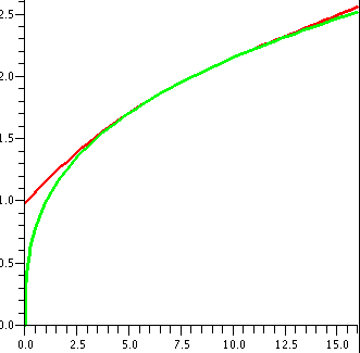 I looked at this error estimate for f(x)=x1/3, n=3, a=8,
and x in the interval [6,8]. I chose an interval centered at 8 so that
|x–8|≤2. To the right is a picture containing graphs of both y=x1/3 and y=T3(x) as x goes from 0 to 16.
Look at the curves. Near x=8, the curves look very, very close. A bit
farther away, the curves separate. Indeed, the best way I can see
which curve is which is that x1/3 goes through (0,0) so
that must be the green curve.
I hope you can see that knowing the polynomial and using it instead of
x1/3 might be advantageous, maybe, maybe (the idea is that
polynomials are very easy to compute and other functions might not
be).
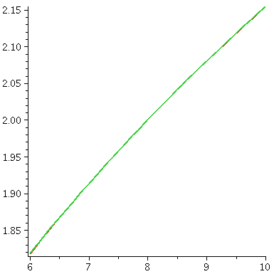 To the right is another picture. Look at it very carefully
please. It is also a graph of both y=x1/3 and y=T3(x) as x goes from 6 to
10. Both curves are displayed. But I can only see one
curve. Maybe if I look really really really closely, maybe I can see
some dots of two colors but I am not sure. How close are these curves?
Well, let's try to use the error estimate in the textbook. That error
estimate is quoted above. So an overestimate of the absolute value of
the difference between T3(x) and f(x) for x in [6,10] is
|Tn(x)–f(x)|≤K[|x–a|n+1/(n+1)!] where K
is some overestimate of |f(n+1)(x)| between x and a.
How can we use this? Well, here f(x)=x1/3 and n=3
and a=8 and the x's involved are between 6 and 10. So we need to
understand K[|x–a|n+1/(n+1)!]. This becomes
K[|x–8|4/4!]. Of course 4! is 24. What about
|x–8|? This is the distance from x to 8. If x is in [6,10], the
largest distance to 8 is 2, so |x–8| is always ≤2. Good: now
we know that the error is at most K[16/24] (because 24 is
16). What about K? To compute K we need f(4)(x). Well, here
are f(x) and a few of its derivatives:
f(x)=x1/3;
f´(x)=(1/3)x–2/3;
f´´(x)=f(2)(x)=–(2/9)x–5/3;
f(3)(x)=(10/27)x–8/3;
f(4)(x)=–(80/81)x–11/3.
I am interested in the absolute value (the size) of the
error, so I will forget the minus sign. Therefore I need to know how
large (80/81)x–11/3 can get on [6,10]. Because of the
negative sign in the exponent, this is a decreasing function of
x, and its largest value is at the left-hand endpoint. So the biggest
this can be is (80/81)6–11/3. O.k.: I gave up -- we
used a calculator. This number is about (rounding up!)
.0014, and I'll take that as my value for K.
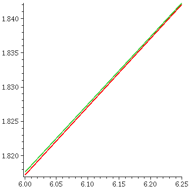 Therefore the error is at most (.0014)(16/24) and this is about
.00092. Now look carefully at the picture. Do you think you can
see a difference in height of less than .001? The difference
between two of the "hashmarks" on the vertical scale is .05, and the
graphs of the functions are separated by one-fiftieth (that's 1/50) of that
difference. I don't think that the pixels in the picture are small
enough to show this!
The picture to the right shown here is on a different interval, from 6
to 6.25 for x. The vertical scale is also different. Each vertical
hashmark here represents a height difference of .001, and now, in the
part of this interval which is farthest away from 8, near 6, I hope
you can indeed see two curves, separated by just a little bit. The error
estimate actually gives useful quantitative information.
We can use the polynomial instead of x1/3 in the interval
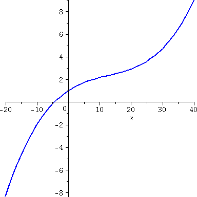
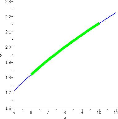
[6,10] and loose little information. Here are two more pictures (yes,
I like pictures, maybe too much). The left picture is just
T3 (it is a cubic polynomial with no critical points [like
x3+x). The right picture has both T3 in blue
again, and a broad "curve" in green of x1/3, with the
latter just shown on [6,8].
|
What are sequences and what are they used for?
A sequence is a sort of ordered list of numbers (precise definition
below).
Much computation is done sequentially. For example better and
better approximations to roots of equations are gotten by Newton's
method. This scheme creates numbers which (ideally!) get closer and
closer to the root desired, even though there may be no exact
algebraic formula for this root. Definite integrals (except in
classrooms!) can only rarely be computed exactly. Instead, there are
usually collections of approximations which are computed, and this
collection of approximations is used to give a "value" for the
definite integral. In this part of the course (really this is the last
major part of the course!) we will study sequences and accompanying
ideas.
Formal definition of a sequence
A sequence is a real-valued function whose domain is the positive
integers. I will begin with what I hope are some rather simple
examples but the later examples will be complicated enough for everyone.
Example and notation
Well, one example of a sequence is a sequence whose nth
term or value or element (all these words are used!) is 1/n. So this
is the function f(x)=1/x when x is a positive integer. The usual
notation for this sequence is {1/n}. Yeah, a different notation is
used -- usually the sequence "function" doesn't get shown. The formula
is enclosed by the braces { and }. The letters that are used inside
the braces are usually n and m and p and q. If needed, we might refer
to the formula with a subscript. So, for example, we might write
an=1/n. Therefore, a5=1/5 and
a17=1/17. Also an+1=1/(n+1) and
a5m=1/(5m). Notice especially the last two equations which
might look strange. The stuff "down" in the subscript is the argument
to the function which defines the sequence. Please try not to get
confused. For example, if an=1/n, then a4=1/4,
but a4+1=a5=1/5 and a4+1=(1/4)+1=5/4.
People also frequently "define" functions by listing their first few
members. So this sequence might look like 1, 1/2, 1/3, 1/4, 1/5,
... and the "..." is supposed to indicate that the reader should now
recognize the pattern. To me this is another use of the strange
mathematical word "clearly". Clearly sometimes people will recognize
the pattern, but also clearly many times there will be difficulty.
I will use some workshop time tomorrow continuing this topic and
catching up with the syllabus.
| Monday, November 2 | (Lecture #16) |
|---|
I discussed the solution to problem #5 of workshop #5. The graphs
involve logistic curves (solutions of a logistic equation) operating
on different time scales (one very fast, and the other very slow. So
here are some pictures and supporting
remarks.
I need to do many more examples, with both pictures and
numbers.
I'll continue with Taylor's Theorem for at least half the lecture on
Wednesday.
|
I wrote this on the board before the class began. It is a result I'll
use several times in the initial discussion. Here:
Suppose we have a differentiable function which is 0 at two distinct points. Then the derivative of
the function will be 0 at least once between
these two values.
Important and useful
Much of the remainder of the semester will be devoted to material
which is extremely useful to everyone involved with engineering and
science. Today is likely to be your first exposure to the ideas which
are generally used to compute values of functions. It is almost
certain that these ideas are at the center of how the calculators and
computers you use compute (and graph) most functions. You should know
something about these ideas.
When I taught this last year I jumped right into an example, and
didn't show people any of the structure. The examples, even the
easiest, can be intricate. I don't feel I was too successful here last
year, so I want to try a different approach today. Some of what I say
will not be in the textbook. I will begin with a totally
unmotivated question. The question will look somewhat weird.
What's K?
Suppose f(x) is a differentiable function, a and b are numbers with
a≠b, and we consider the equation:
f(b)=f(a)+f´(a)(b–a)+[f´´(a)/2](b–a)2+K(b–a)3.
Then there is some number K which makes this equation
correct. Why? Because since a≠b, (b–a)3 isn't 0, and I
could solve for K in this whole messy equation. So I want to
investigate what K is, and get another way of writing K. To do this I
will use the Mean Value Theorem repeatedly in the form quoted above.
Consider the function
G(x)=f(x)–(f(a)+f´(a)(x–a)+[f´´(a)/2](x–a)2+K(x–a)3).
What do I know about G(x)? Well, I know that G(a)=f(a)–(f(a)+f´(a)(a–a)+[f´´(a)/2](a–a)2+K(a–a)3) so that G(a)=0. I also know that G(b)=f(b)–(f(b)+f´(a)(b–a)+[f´´(a)/2](b–a)2+K(b–a)3). This is also 0 because K was chosen so that this
is true. So G(a)=0 and G(b)=0. Therefore (MVT/RT above) there is
some number in between a and b, I'll call it c1, so that
G´(c1)=0.
Now let's compute the derivative of G(x). There are many letters
around. I am differentiating with respect to x. With this in mind, I
see:
G´(x)=f´(x)–(0+f´(a)1+[f´´(a)/2]2(x–a)+3K(x–a)2).
Now what? Well, G´(a)=f´(a)–(0+f´(a)1+[f´´(a)/2]2(a–a)+3K(a–a)2) is 0 because of the a–a's and because the
f´(a)'s cancel. We also know that G´(c1)=0. Now
MVT/RT applied to the function G´(x) tells us that its derivative
is 0 somewhere between a and c1. That is, there is
c2 between a and c1 so that
G´(c2)=0.
Now let's compute the derivative of G´(x), again being
careful.
G´´(x)=f´´(x)–(0+0+[f´´(a)/2]21+3·2K(x–a)).
Of course we consider G´´(a) which is
f´´(a)–(0+0+[f´´(a)/2]21+3·2K(a–a)) and this is 0. Also G´(c2)=0. So
MVT/RT again applies to tell us that there is c3 between a
and c2 with G´´´(c3)=0. Wow.
The derivative of G´´(x):
G´´´(x)=f´´´(x)–(0+0+0+(3·2·1)(K)1).
Now we know when x=c3 this is 0. So we know that
f´´´(c3)–(3·2·1)K is
actually equal to 0. We can
solve this for K, and get
K=[f´´´(c3)/(3·3·1)].
c3 is between a and c2 and
c2 is between a and c1 and
c1 is between a and b so that c3 is itself
between a and b.
What's going on?
Here is what we know: If
f(b)=f(a)+f´(a)(b–a)+[f´´(a)/2](b–a)2+K(b–a)3.
then there is a number c between a and b so that
K=[f´´´(c)/(3·2·1)] (three of the ´
in this). This turns out to be
the beginning of a marvelous and successful computational strategy.
So what's your problem with all this? You might claim to not
understand what the heck is going on, and, more particularly,
why any moderately sane person might want to go through these
algebraic contortions. Yes I totally agree with
you. But it turns out (sit here, look at the fireworks (?) that
follow) this is extremely useful. There have been centuries
(!!) of thought involved in preparing and using all this stuff -- it
is really clever.
Taylor polynomials
This is copied from page 502 of your text. The Taylor polynomial of degree n for the function f(x)
centered at a (wow, what a collection of words!) is
Tn(x)=f(a)+f´(a)(x–a)+[f´´(a)/2](x–a)2+[f(3)(a)/3!](x–a)3+...+[f(n)(a)/n!](x–a)n
There are a whole bunch of things to discuss. Let's see. First, if
you've never seen it before, the appearance of the excitement
mark, !. This is called a
factorial. The value of the factorial of a positive integer is the
product of the integer together with all of the integers less than it
down to 1: n!=n(n–1)(n–2)(n–3)···(3)(2)(1). Here is a very brief table of factorials:
| n | 1 | 2 | 3 | 4 | 5 | 6 | 7 | 8 | 9 | 10 |
|---|
| n! | 1 | 2 | 6 | 24 | 120 | 720 | 5,040 | 40,320 | 362,880 | 3,628,800 |
|---|
The major thing you should notice right now is that the factorials
grow very big very quickly. That's computationally important. I also
should mention that most people define 0! to be 1. That's so
certain formulas are easier to write (really). (It turns out to be
possible to define factorials of other numbers. For example, in 251,
you can define and compute (1/2)! -- wait for
that.)
More notation is in such things as f(4)(a). This means the
fourth derivative of f evaluated at a. So f´´(a) can also be
written as f(2)(a), and even just f´(a) is
f(1)(a). Again, in order to make writing certain formulas
easier, most people think that f(0)(a), the zeroth
derivative of f evaluated at a (so no derivatives are done!), should
just be f(a).
If all of this notation is clear, then here's another, very compact
way to write the Taylor polynomial.
Tn(x)=∑j=0n[f(j)(a)/j!](x–a)j.
I hope you can see where the zero factorial and zeroth derivative make
this much easier to write.
Example 1
Let's get T8(x) for sin(x) and a=0. So we need derivatives, and here they are:
| Derivative # | Function | Value at a=0 |
|---|
| 0 | sin(x) | 0 |
| 1 | cos(x) | 1 |
| 2 | –sin(x) | 0 |
| 3 | –cos(x) | –1 |
| 4 | sin(x) | 0 |
| 5 | cos(x) | 1 |
| 6 | –sin(x) | 0 |
| 7 | –cos(x) | –1 |
| 8 | sin(x) | 0 |
The numbers in the last column, together with the factorials, are the
coefficients which build the Taylor polynomial. I emphasized with all
of these examples that noticing patterns is the way to go. In the case
of sine, the derivatives repeated every four. I am not cheating
by choosing something excessively simple. Almost every function I know
that arises in modeling physical and geometrical situations has
patterns in its derivatives, and part of the fun (?) is finding these
patterns. Well, now I can write T8(x):
T8(x)=[0/1](x–0)0+[1/1](x–0)1+[0/2](x–0)2+[–1/6](x–0)3+[0/24](x–0)4+[1/120](x–0)5+
+[0/720](x–0)6+[–1/5,040](x–0)7+[0/40,320](x–0)8
Only a nitwit or a very pedantic math instructor would write it that
way. Most people would drop the 0 terms, change (x–0) to x, make a few
other notational simplifications,and get
T8(x)=x–[1/6]x3+[1/120]x5+[1/5,040]x7
Then there are some questions.
What is T4(x)? It must be
x–[1/6]x3.
What is T7(x)? It
must be
=x–[1/6]x3+[1/120]x5+[1/5,040]x7,
in this case just the same as T8(x).
What is
T10(x)? I bet it is the same as T9(x), and this
would be
T10(x)=x–[1/6]x3+[1/120]x5+[1/5,040]x7–[1/362,880]x9.
Graphs of sin(x) and
T9(x)=x–(1/6)x3+(1/120)x5–(1/5040)x7+(1/362880)x9
on the interval [–8,8].
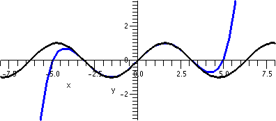 So I'm skipping a few polynomials and jumping up to the 9th
degree approximation. The numbers may look a bit strange (you will
get used to them!).
By now doing numerical computations is almost silly, but here is the
value of the 9th degree polynomial at x=1: it is
0.8414710096. This agrees with the true value of sin(1) to 6 places
(rounded). At x=.5, the approximation and true value agree to 10
decimal places.
Let me explain why T9(.5) and sin(.5) agree to so
many decimal places. Well, we need a generalization of the first
computation we did. Here is the result, a version of what's called
Taylor's Theorem:
If
Tn(x)=∑j=0n[f(j)(a)/j!](x–a)j,
then the difference between this and f(x) is
[f(n+1)(c)/(n+1)!](x–a)n+1 for some c between a
and x.
This is the error or remainder. In the case of sine and n=9, we need
to estimate
[f(n+1)(c)/(n+1)!](x–a)n+1 when a=0 and
x=.5. Well, the 10th derivative of sine is sine or –sine or
cosine or –cosine, and in any case the absolute value can't get bigger
than 1. So an overestimate of the absolute value of the error:
[f(n+1)(c)/(n+1)!](x–a)n+1
when a=0, x=1/2, and n=9 becomes [1/(10!)](1/2)10 and this is
[1/3,628,800](1/1,024) which is less than 10–10. That's
where the 10 place accuracy comes from.
Example 2
We get T8(x) for f(x)=ex and a=0.
| Derivative # | Function | Value at a=0 |
|---|
| ....blah.......blah.......blah.......blah.......blah..........blah... |
|---|
| any n you want! | ex | 1 |
| ....blah.......blah.......blah.......blah.......blah..........blah... |
|---|
T7(x)=1+x+[x2/2]+[x3/6]+[x4/24]+[x5/120]+[x6/720]+[x7/5,040]
It's supposed to be easy: this is a technique people actually use.
How good is T7(–.4) as an approximation to e–.4?
Here the remainder is
[f(n+1)(c)/(n+1)!](x–a)n+1
when a=0, x=–.4, and n=7 becomes
ec[1/(8!)](–.4)8. Now c is between –.4 and 0 and
since ex is increasing, the biggest value occurs at c=0,
where e0=1. (It is supposed to be easy, otherwise
people would not use it!) So the error is at most
[1/(8!)](–.4)8. This is less than .00000002.
The "true value" of e–.4 is 0.670320046035639
the value of T7(–.4) is 0.670320030476191. I had a machine
do these computations, of course. The reason I put quotes around "true
value" is that the machine used Taylor polynomials to do the
computation, of course.
| Wednesday,
October 26 | (Lecture #15) |
|---|
Story #3
A hot object is brought into a room whose ambient temperature is
30oC. After 10 minutes, the temperature of the object is
measured and found to be 80oC. After another 10 minutes (20
minutes from the start) the object's temperature is 40oC. What
was the initial temperature of the object? What is the temperature of
the object an hour after it was brought into the room?
Assume that the rate of temperature change is directly
proportional to the difference of the temperatures. (This is
Newton's Law of Cooling whose validity can be checked
experimentally.) The "room with ambient temperature" is what's called
a heat sink. The assumption is made that the totalheat of the
object isn't enough to really change the room's temperature. Many
devices rely on similar assumptions, which may be valid.
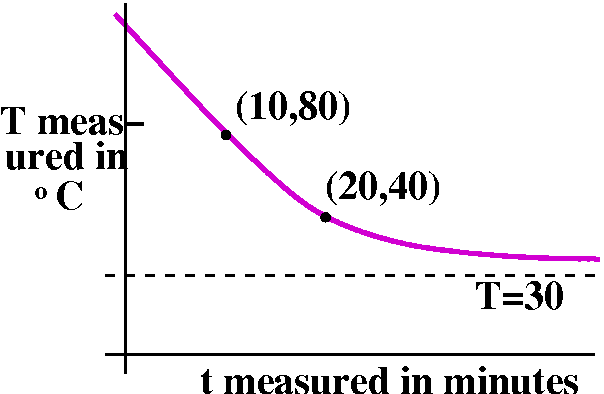 Modeling this story to solve the problem
Declaring that the quantity FROG is directly
proportional to the quantity TOAD is language meaning
that FROG=KTOAD for some positive constant K. So if
T represents the temperature of the hot object, then Newton's Law of
Cooling implies that RATE OF CHANGE OF T=K(difference
between T and 30). With the usual notation, realizing that "rate
of change" is a derivative, and using T in oC and t for
time measured in minutes since the object was brought into the room,
Newton's Law of Cooling becomes dT/dt=K(T–30) with some unknown
constant, K. What about the other information in the story? I've
collected the information in a possible graph of the temperature of
the object to the right. Our guess for the solution curve (the
description of the temperature as time changes) is in magenta. It should tend to 30 as t→∞.
Solving the model equation
dT/dt=K(T–30) is separable, so we get (I'm beginning to skip steps)
∫[1/(T–30)]dT=∫K dt so that ln(T–30)=Kt+C. We
have two constants, K and C, to be determined. But we know two
"chunks" of information about the temperature, (10,80) and
(20,40). Therefore (plugging in):
(10,80) gives us ln(50)=K(10)+C
and (20,40) gives us ln(10)=K(20)+C.
We have two linear equations in two unknowns. We can solve them. Use
your favorite method, or:
Double the first equation and subtract the second to get
2ln(50)–ln(10)=C. I will simplify using log properties, so
C=2ln(50)–ln(10)=ln({50}2)–ln(10)=ln(2500)–ln(10)=ln(250).
Let's put this value of C in the first equation. We have
ln(50)=K(10)+ln(250) so 10K=ln(50)–ln(250)=ln(50/250)=ln(1/5) and
K=(1/10)ln(1/5).
The solution and the solution curve
 The implicit form of the equation is therefore
ln(T–30)=(1/10)ln(1/5)t+ln(250). Let's exponentiate, and use
exponentiation properties and log properties:
T–30=e(1/10)ln(1/5)t+ln(250)=e(1/10)ln(1/5)teln(250)=eln[(1/5)(1/10)t](250)=250(1/5)(1/10)t, and, finally,
T=250(1/5)(1/10)t+30 or maybe 250(5–(1/10)t)+30. Whew!
Please note that on an exam I would not require or expect so much
"simplification" but when you go out and work on such problems, people
usually like the answers written in such "simple" ways. Since
T(t)=250(1/5)(1/10)t+30, the initial temperature, T(0), was
250+30=280. The temperature after one hour is T(60) (60 minutes=1
hour) and that is 250(1/5)6+30 which is 30.016 (no, I did
not compute this!). Also please note that as t→∞, since
(1/5) is a positive number less than 1,
250(1/5)(1/10)t→0 so that T(t)→30 as we had
guessed.
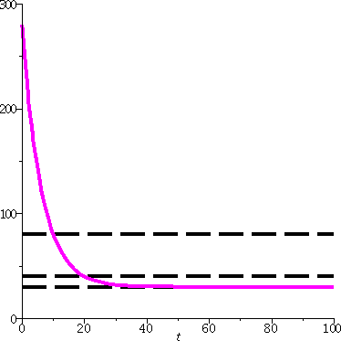
To the right is a graph of T(t)=250(1/5)(1/10)t+30 in magenta with dashed black lines at 80, 40, and
30. The 80 and 40 lines cross at 10 and 20, respectively, and the
curve overlays the 30 line as t grows. The curve seems to cross
the t=0 line at T=280.
Bacteria again ...
The differential equation dy/dx=Ky with K constant (so the solutions
can be written as y=CeKx) is widely used for modeling drug
levels in blood and radiocarbon dating (K negative) and for modeling
growth of bacteria, yeast, fungus, etc. when K is positive. x is
usually time. How valid is this? Well, if we had E. coli which would
"divide every twenty minutes" we should be 50 feet under E. coli even
if the darn things started only a few weeks ago. In fact, for such
growth there are limits to nourishment and other factors which retard
growth as the population increases. Sometimes such things are bundled
into the model as the "Carrying Capacity" of the system. So people
have considered many differential equations which model growth. Let me
discuss a very simple case of a widely accepted model equation.
A better model: the logistic equation
Consider the
differential equation dy/dx=y(2–y). If y is close to 0 but
positive, then the right-hand side seems to be about "2-ish"
multiplying y. So this is very much like dy/dx=2y, exponential
growth. If y is close to 2 but less than 2, then dy/dx is (really
small number) multiplying y, so y will grow very slowly. Therefore 2
serves as the Carrying Capacity of this model. I will try to solve a
specific initial value problem for this equation, which is an example
of the Logistic Differential Equation. The numbers are
selected to make the algebra as easy as possible.
The initial value problem will consist of the differential equation
dy/dx=y(2–y) and the initial condition y(0)=1.
- Separate and integrate:
∫[1/{y(2–y)}]dy=∫dx.
- The left-hand side needs partial fractions:
[1/{y(2–y)}]=(z/y)+(w/{2–y}) so (tops only) 1=z(2–y)+wy. y=0 gives
z=1/2 and y=2 gives w=1/2. Now integrate.
- (1/2)ln(y)–(1/2)ln(2–y)=x+C where the minus sign before one of the
1/2's comes from the antiderivative of 1/(2–y). If x=0, y is supposed
to be 1. Then (1/2)ln(1)+(1/2)ln(1)=0+C so C=0 ("select the numbers
to make everything as easy as possible").
- The solution implicitly is therefore (1/2)ln(y)–(1/2)ln(2–y)=x but
people like explicit forms. So multiply by 2 and use the ln property
to get ln(y/{2–y})=2x. Exponentiate so y/{2–y}=e2x. We need
still to solve for y. Multiply by 2–y and
y=e2x(2–y)=2e2x–e2xy and
y+e2xy=2e2x and
y(1+e2x)=2e2x. Huh. So clearly ...
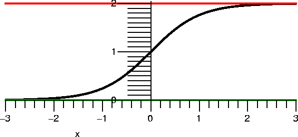 An explicit form of the solution is
y=[2e2x]/[1+e2x]. This may be in a form that
"real people" can understand.
A picture of this curve is shown to the right. The curve does pass
through (0,1). For t negative, the curve does sort of look
exponential. When t is large enough (t=0 in this case), the concavity
of the curve flips (it is always increasing!) and as t→∞, y→2. 2 is sometimes called the
carrying capacity of this "system". This function is sometimes
called (a version of) the logistic function.
But what happens if ...
What if we wanted to look at a different, even just slightly more
complicated model, say dy/dx=y(y–1)(y–2) etc. Then separating etc. is
possible. But trying to convert the implicit description of the
solution to an explicit description, one that can be analyzed more
easily, is essentially impossible unless we are very lucky.
A different kind of reasoning
There is a different way to study such equations, one where geometric
reasoning is used instead of lots of algebraic computations. When this
sort of reasoning applies, getting asymptotic information is usually
much easier than one would think possible. The tool we will consider
for this way of studying differential equations is called the
direction field in your textbook (in others it is called the
slope field). I will use this tool to get an approximate idea
of the shape and behavior of what are called solution curves or
integral curves of the differential equation. These are the
graphs of particular solutions of the differential equation.
Direction fields
Let's look at the differential equation
y´=x2–x–4y2. I can't "solve" this but let
me tell you just a small amount of information about the solution near
the point (3,1). A solution curve passing through the point (3,1) will
have its slope determined by the differential equation. I mean that
y´ when x=3 and y=1 will be the value of
x2–x–4y2 when x=3 and y=1. This is
32–3–4·12=9–3–4=2. So the tangent line to
the curve at (3,1) will have slope 2. Well, let's think about it. I'll
draw a thickened-up line segment of slope 2 at (3,1) and consider some
curves going through that point.
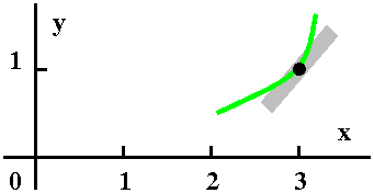
| Curve #1 I've drawn a little piece of
a curve, tangent to the chunk of line (it is formally called a line
element, I think). I think this curve, which is increasing, might
possibly be a solution to this differential equation near this point.
A possibility
|  |
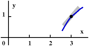
| Curve #2 Here is another curve going
through (3,1). I believe that this could also be the solution
curve. O.k.: it is concave down, and I surely don't know what the
concavity of the solution curve is at (3,1) without more study. But in
my casual way, I have two possible candidates for the solution
curve. Certainly it is also increasing near (3,1) because the slope at
(3,1), which is 2, is positive.
A possibility
|  |
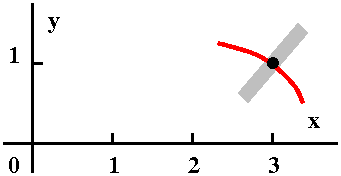
| Curve #3 Now this candidate is really
a different sort of curve. This curve does pass through (3,1) but it
is decreasing, and its slope is certainly not 2 at (3,1). This is a
losing candidate (!) and certainly can't be a little piece of
a solution curve.
Not possible!
|  |
I don't think that this "reasoning" is profound. I am merely asserting
that I can eliminate and (tentatively) accept certain candidate curves
as good candidates for solution curves. Now I will extend the
reasoning, by drawing lots of line segments at lots of points and see
what my brain's visual processing power can tell me about the
curves. In fact, (and this is somewhat amazing to me) with some
practice, most people can "see" the curves quite clearly. So here are
some examples. The direction fields were drawn by computer, but the
curves were (badly) drawn by me. In class, I was so proud of our boys
and girls who did not quarrel about the crayons!
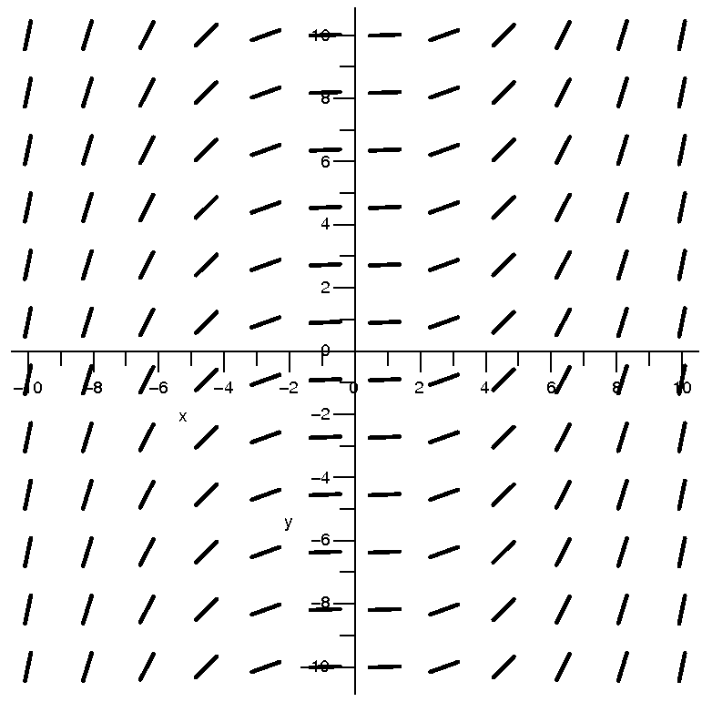
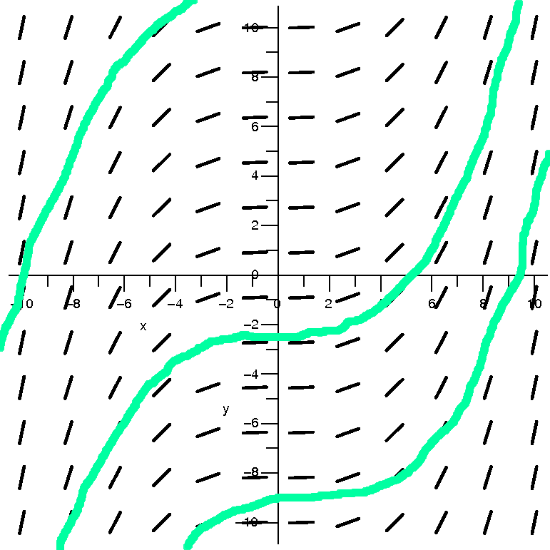
| dy/dx=(1/20)x2 |
| This is the direction field |
This is the direction field with
some solution curves. |
|---|
|
|
Discussion
I had Maple draw a bunch of direction
fields. I admit that the instructions took a bit of practice, but once
I understood them it wasn't too difficult to produce the pictures, and
I honestly tell you that there was a great deal less computation than
if I had requested any approximations to solution curves
numerically. There are 12·12=144 line elements in each
direction field picture. The rather strange numbers which appear in
the differential equations (for example, the (1/20) in this equation)
were chosen so that the tilts of the direction field elements would be
easier to see in these pictures.
This differential equation can be solved easily and its solutions are
(1/20)(1/3)x3+C. But I want to
look at the curves and not the formulas. Here to the left is
the direction field without any decoration. To the right is my attempt
to draw by "hand" curves which, whenever they touch a line element,
have the line elements as segments of tangent lines. I think you can
see that the solution curves are increasing, and that the concavity is
down on the left and up on the right. That's all I want from this
example.
|
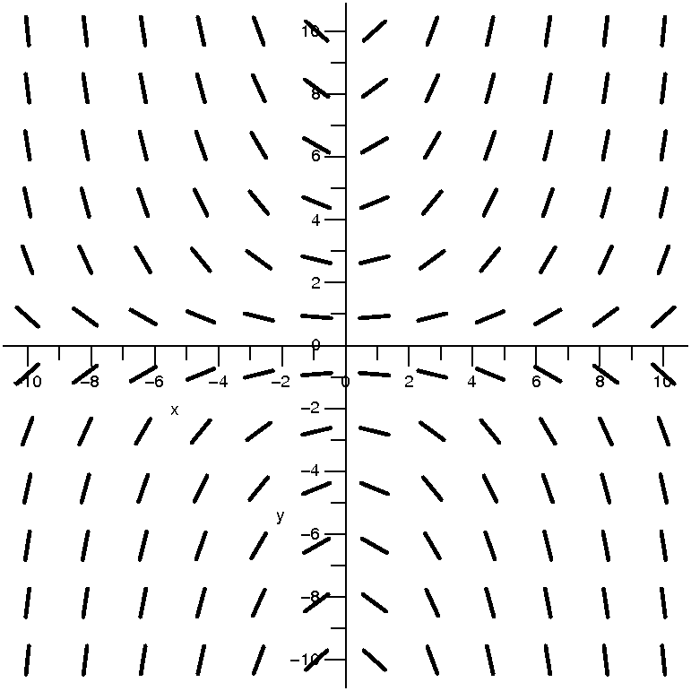
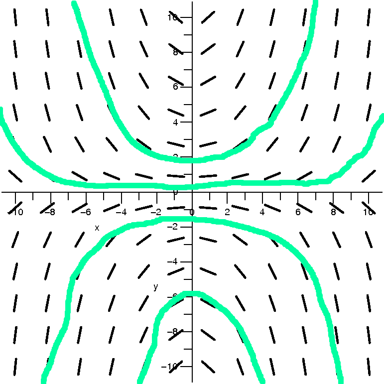
| dy/dx=(1/10)xy
|
| This is the direction field |
This is the direction field with
some solution curves. |
|---|
|
|
Discussion
O.k., algebraically this differential equation is still something we
can handle fairly easily. This is a separable equation, and we can
solve it fairly easily. Let me take the 144 pieces of the direction
field and try to draw some curves which, when they touch any
part of the direction field, will have that tiny line segment looking
like it is tangent to the curve. To me these words more make things
harder to understand. Draw some curves!
The curves I "drew" are concave up when they are above the x-axis, and
they are concave down when they are below the x-axis. I feel that I
understand how initial conditions would "evolve" (?) forward and
backward. People frequent thing that x is a variable representing
time. So an initial condition located in the upper halfplane, above
the x-axis, evolves forward (the future) and gets very very
large. Also, in the past, it came from something very very
large. That's all I want here: just approximate
qualitative information about
solutions.
There is one special solution curve (not drawn here) which is the
x-axis, with y=0. You can check that y=0 is a solution of this
differential equation. The y values don't change. Such a solution is
called an equilibrium solution.
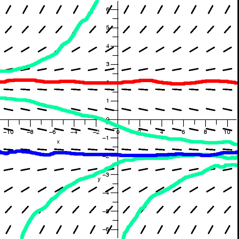
|
| dy/dx=(1/30)(y+2)(y–2)
|
| This is the direction field |
This is the direction field with
some solution curves. |
|---|
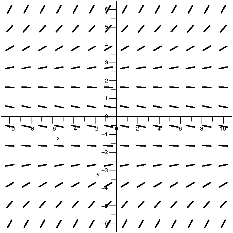
|
|
Discussion
I can still solve this algebraically, I think (I haven't tried). This
is a variant on the logistic equation which has a nicely worked out
solution above. Here the numbers are a bit more random, though. The
direction field tells me more in a short amount of time than working
algebraically would tell me in a long time.
Look at the picture of the direction field, and then look at the
solution curved indicated. There is a great deal going on in the
picture of the curves, and let me try to pick out some features.
First, there are some horizontal lines which are
solutions. How can I detect them? If y=Constant is a solution to some
complicated differential equation dy/dx=F(x,y), then
because the horizontal line always has dy/dx=0, it had better be true
the the complicated function F(x,y) is 0 when we plug
"Constant" in for y. This may seem complicated to you, but here look
at the right-hand side: (1/30)(y+2)(y–2). When is this equal to 0?
Without being silly, I think I can write that clearly this occurs for
y=–2 and y=+2. The horizontal lines defined by these questions are
then solutions to the differential equation dy/dx=(1/30)(y+2)(y–2)
because both sides are 0. These solutions don't change with "time" if
we think of x as time. Here is some vocabulary which is used when
discussing these solutions: they are called equilibrium
solutions or steady-state solutions.
Please also note that the two equilibrium solutions divide the plane
into three chunks. A solution curve which starts in one chunk
can't go into a different one. It would have to cross one of
the equilibrium curves, and, at that crossing point, there would be
two solution curves, which would contradict the Existence and
Uniqueness Theorem. For in that theorem is the assertion
that each point has at least a little piece of exactly one, only one,
solution curve.
Now I want to discuss other (non-equilibrium) solutions for this
differential equation. Consider first solutions near the equilibrium
solution y=–2. If we take initial
conditions (x0,y0) with y0 not
equal to –2 but near –2, something interesting
happens. The curves above y=–2 get moved down as we go futureward (x
increases). They get moved down towards –2, and as close to –2 as you
want (yes, a limit indeed). And if y0 is below or less than
–2, the curves below y=–2 move up towards –2. More precisely, if we
take an initial condition (x0,y0) with
y0 close to –2, the resulting solution y=f(x) has the
property that limx→∞f(x)=2. Nearby solution curves converge to the
equilibrium solution y=–2. This situation has its own name: y=–2 is
called a stable
equilibrium. There are many physical situations
(mechanical, chemical, etc.: many!) where learning about stable
equilibriums (equilibria?) is very important. In real life,
determining an exact measurement (y=–2) may be very difficult. It is
far better to know that, hey, starting something off near –2
will have the same long-term effect as starting it at –2. This is
useful and neat.
Let's look more closely at the other equilibrium solution,
y=2, and its neighboring solution
curves. Suppose we start near but above y=2. If you look at
the picture, you'll see that the direction field pushes (?) the curve
away from y=–2 (these curves go to ∞). Similarly, if we start near but below y=2, the curves get
pushed away from y=2. The lower curves go towards y=–2, which right
now is not interesting: I want to concentrate are things near y=2. So
if this differential equation described a physical situation, I would
now know that if my initial condition (x0,y0)
had y0 exactly at 2, then on the solution curve, I would
have y0 always equation to 2 as x0 increased
(the future). But if I didn't get y0 exactly equal
to 2, I have no ability to predict the future. Maybe y will tend to
∞ or maybe to –2. Here's the
vocabulary, which shouldn't be surprising: y=2 is called an unstable equilibrium.
|
Physical situation
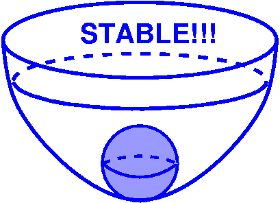 Stable equilibrium
Think of a ball at the bottom of a bowl. It will just sit there,
position not changing. If you jiggle the bowl a bit, then the ball
will move, but eventually (if you stop jiggling) it will go towards
the bottom again. This "bottom" situation is a stable
equilibrium.
|
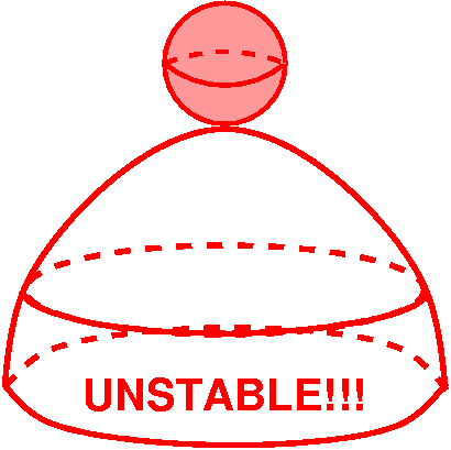 Unstable equilibrium
Turn the bowl over and put the ball on top of the bowl. You may
conceive of a situation where you have placed the ball so carefully on
the top that is it totally balanced and still, motionless. Ideally the
situation would go on forever -- equilibrium. But now jiggle the ball
in any way, with a very small jiggle, in any direction. The ball will roll
off. This is unstable equilibrium.
|
|
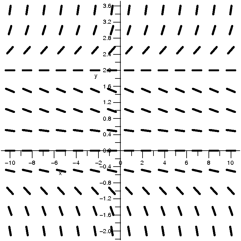
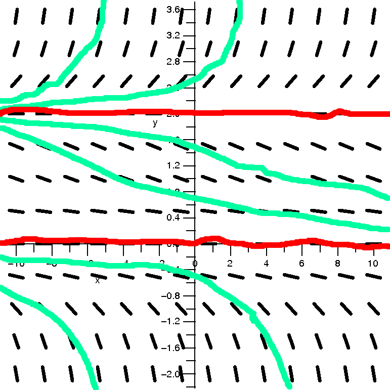
| dy/dx=(1/30)y2(y–2)
|
| This is the direction field |
This is the direction field with
some solution curves. |
|---|
|
|
Discussion
O.k.: I definitely would not want to try to "solve" this
equation algebraically and get explicit solutions. But the direction
field approach combined with simple reasoning allows me to find
equilbrium solutions and even to detect which are stable and which are
unstable, and this can be very useful in practice.
I diagnose equilibrium solutions by considering
(1/30)y2(y–2)=0. The roots are 0 and 2. So y=0 and y=2 are
the only equilibirum solutions for this differential equation. Yes, I
admit it: this example is very carefully chosen so that the method
works, but the ideas are sufficiently nice so that the method will
work even for examples which aren't so "pretty".
What about stable and unstable? Again, look at the direction field,
and then examine the solution curves which are drawn. Both of the
equilibrium solutions are unstable. Nearby solution curves are not
"sucked into" the equilibrium solution. Yes, it is true that curves
above y=0 get pulled towards y=0, but to be an equilibrium solution,
both sides (up and down) must have solution curves which are attracted
to the equilibrium, and this does not occur here. Again, both of these
equilibrium solutions are unstable.
Mr. Priestner commented that the
equilibrium solution y=2 sort is is stable when "time" (x) runs
backwards, that is, as x→-∞. My comment was that certainly
it was true that y=2 attracts solutions, but the word "stable" is
usually reserved only for solutions which are attracting as
x→+∞, so y=2, in that standard sense, is not stable.
|
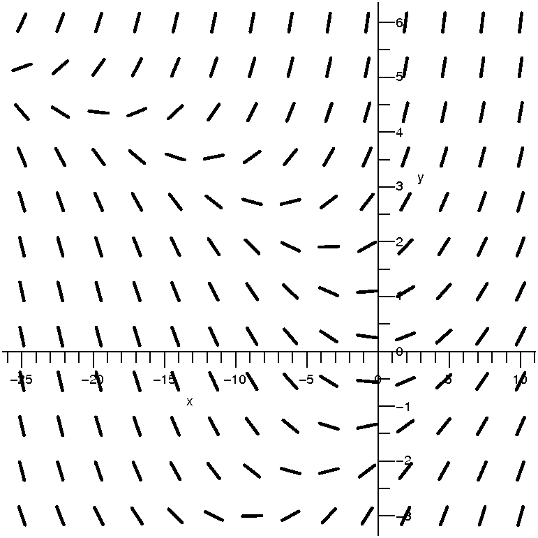
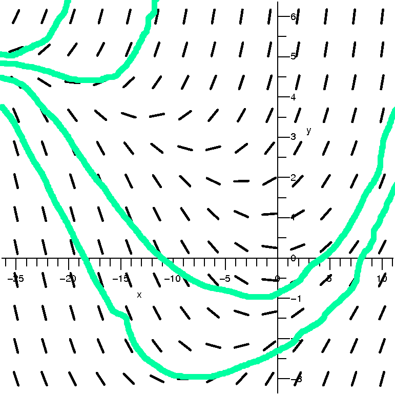
| dy/dx=(1/20)(x+y2)
|
| This is the direction field |
This is the direction field with
some solution curves. |
|---|
|
|
Discussion
O.k., the last example for this method is really nearly random. The
right-hand side, (1/20)(x+y2), is a low-degree polynomial,
but I don't know how to solve the equation (see the remark below if
you are curious, though!). There are no equilibrium solutions because
there is no constant C which makes (1/20)(x+C2) equal to 0
for all values of x. So here's a complicated situation. But still,
consider the direction field, which is easy to have drawn, needing
very little computational effort. And consider the curves I drew. I
bet that the following occurs: if y=f(x) is a solution to this
differential equation, then there will be exactly one critical point
on the solution curve, and this critical point will be an absolute
minimum. To the right of the solution curve, the function will
increase. In fact, it will explode in finite time, that is,
there will be some Q so that
limx→Q–f(x)=∞, but I don't think the picture necessarily tells that. What
about to the left of the solution curve? I bet that somewhere the
concavity of the solution changes, and it becomes concave down, and
that the curve sort of tapers off to a sort of flat situation.
Everything predicted here is actually correct. It would be rather
difficult (but possible, I think, but I wouldn't want to do it!) to
confirm all this algebraically. I think the direction field idea is
worth using as a tool when analyzing differential equations,
especially when some quick asymptotic information is wanted.
|
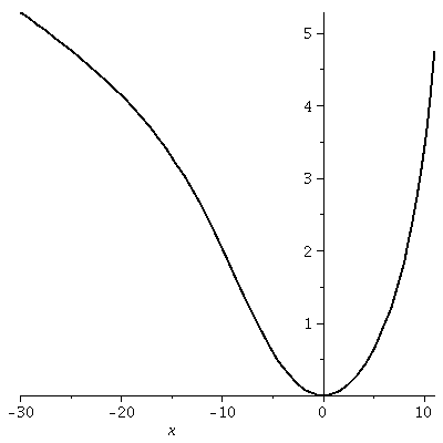
The real thing
Much computation is needed to produce an "explicit" solution
to dy/dx=(1/20)(x+y2). To the right is a picture of the
solution curve which goes through (0,0). The function defining the
curve can't be written in terms of the standard functions you
know. The rather
simple-looking picture is the result of a bunch of Airy functions
combined in very strange ways. I am not inventing all this! The
situation is very complicated.
Here is the solution in detail, written by a silicon friend of mine: 2/3 2/3
50 x (2/3) 50 x (1/3) (1/6)
AiryAi(1, - -------) 150 + 5 AiryBi(1, - -------) 20 3
100 100
1/5 ---------------------------------------------------------------------
2/3 2/3
50 x (2/3) 50 x (1/6)
AiryAi(- -------) 3 + AiryBi(- -------) 3
100 100
I don't understand this complicated formula at all. But I
do understand the direction field and the solution curves.
|
|
A possible QotD
As usual, there wasn't enough time. But if there had been, I would
have asked the following question.
Find the solution of y´=(ex/3)/y which satisfies
y(0)=2. Be sure to write the equation as y=some function of x. Here is a solution which you should look at
after you try the problem yourself.
| Monday,
October 26 | (Lecture #14) |
|---|
Please bring some drawing implements to class on Wednesday since we
will all draw pictures then, together. Isn't that nice?
What's a differential equation?
A differential equation is an equation relating an unknown function
and one or more derivatives of the unknown function with some other
functions.
Examples
y´=x2 Done in 151 (Rutgers Calc 1) ; to be reviewed here.
y´=5y Done in 151 (Rutgers Calc 1) ; to be reviewed here.
y´=y2 We'll discuss this here.
y´=xy We'll discuss this here.
y´=x+y To be discussed in your differential equations course.
y´´=–y To be discussed in your differential equations course. This equation
governs simple harmonic motion (the movement of an ideal
vibrating spring).
y´=x2+y2 This can't be "solved" in terms of
standard functions.
Order of a differential equation
This is the highest numbered derivative which occurs in the
differential equation. In these two lectures we will look only at
first order equations. All of the examples above are first
order, except one (the simple harmonic motion equation) which is
second order. Please note that the differential equations course which
most of you will take will indeed study equations of higher order, and
that these do occur. Some standard vibrating beam equations studied in
mechanical engineering are fourth order, and many of the equations in
physics and chemistry are second order.
Story #1
Probably we have all been told that bacteria (usually) reproduce by,
say, binary fission. This is more or less correct, and more or less
the fact means that the rate of increase of bacteria at any time is
directly proportional to the number of bacteria at that time. So twice
as many bacteria "now" means that twice as many bacteria are being
born now. This is certainly dreadfully simplified, but this
approximation works in many circumstances. I wondered, when I first
heard this fact, why, if, say, E. coli doubles rather rapidly,
shouldn't the world be covered very soon by a layer of E. coli which
is 40 feet thick? In fact,
A single cell of the bacterium E. coli would, under ideal
circumstances, divide every twenty minutes.
(From Michael Crichton (1969) The Andromeda Strain, Dell, N.Y. p.247)
But of course anything growing so rapidly in the real world (mold in a
petri dish) enters a situation where the growth challenges the ability
of the environment to support the thing. Most environments have a
carrying capacity -- some sort of upper limit to the amount of the
thing which can live in the environment. Differential equations can
model this sort of situation fairly well, combined with the
"exponential growth". But exponential growth was studied in calc 1,
and the equation y´=5y sort of models unrestricted exponential
growth.
Story #2
We start with an 800 gallon tank of pure water. It is being filled
with a fluid at 50 gallons per minute, and these 50 gallons contain 5
lbs of salt. At the same time, 50 gallons per minute of the solution
in the tank is being drained. How much salt is in the tank at any
time? How much salt would you expect to be in the tank after a long
time?
Let's construct a differential equation which models the salt in the
tank. We'll call S(t) the number of pounds of salt in the tank at time
t. How much salt is being added? Well, 5 pounds per minute. How much
salt is being taken away? This is more subtle, and we had some
discussion of our assumptions during class. The simplest analysis,
which we will do here, is to assume that the tank contents are mixed
well: it is homogeneous. The situation with a large real tank might
not match this, of course. But, actually, real containers and tanks
sometimes have mixing devices installed to try to match this
assumption. Well, if there are S(t) pounds of salt in the tank at time
t, and if the tank holds 800 gallons, and if 50 gallons are taken out,
then the proportion of 50/800 of the salt is taken out:
[1/(16)]S(t). Now we put things together.
dS/dt, the rate of change of the salt, is +5–[1/(16)]S(t). The
differential equation is dS/dt=5–[1/(16)]S. We also shouldn't forget
that we start with no salt at all in the tank: S(0)=0.
Prediction? What should happen over the long term to the amount
of salt in the tank? It starts out at 0, and then increases ... to
what? Well, a guess is that the amount of salt in the tank
should increase to 80 pounds, which is the same as the salt
concentration (1 pound per 10 gallons) incoming. We will see how to
solve the differential equation and check this prediction.
The solution is discussed here.
Solution of a differential equation
A solution of a differential equation is a function which, when it and
all of its relevant derivatives are inserted into the differential
equation, makes the equation true for all values of the domain
variable. I know this may seem long-winded, but I hope the discussion
and examples which follow will shown why such elaboration is
necessary.

An example: y´=x2
Well, we know how to solve y´=x2: just integrate. We
did this repeatedly last semester (and even this semester). The
solutions are y=(1/3)x3+C, where C is any constant. There
are infinitely many solutions. A few of them are shown to the right.
The blue curve has C=1: y=(1/3)x3+1. It
is the solution curve which goes through (0,1).
The red curve has C=3: y=(1/3)x3+3. It is
the solution curve which goes through (0,3).
The green curve has C=–2:
y=(1/3)x3–2. It is the solution curve which goes through
(0,–2).
The solution curves are just vertical translates, up and down, of each
other. They are all the same shape, have the same domain, etc. This
situation is rather straightforward, as you will see.
General solution; particular solution
There is some special vocabulary used. The differential equation
y´=x2 has the general solution
f(x)=(1/3)x3+C. When C has a specific value, then the
function is called a particular solution. So
f(x)=(1/3)x3–2 is a particular solution, and it is the only
particular solution which passes through (0,–2). The specification
(0,–2) is called an initial condition. That comes from the
physical situation where x represents time, and we think that the
y-value corresponding to the given x-value represents a certain
starting place. Sometimes people write y(0)=–2 as the initial
condition. That can confuse me. The combination of an initial
condition and a differential equation is called an initial value
problem.
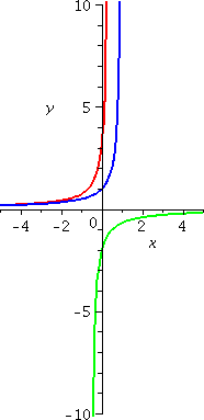 An example: y´=y2
Now let's change and consider y´=y2. I guess
that the general solution is f(x)=1/(C–x). (I'll show you how to
guess it also, very soon!) How could you check that my suggestion for
a solution actually is a solution? Well, if f(x)=1/(C–x) then,
since f(x)=(C–x)–1, we know that
f´(x)=(–1)(C–x)–2(–1). The first –1 comes from the
power, and the second –1 comes from the Chain Rule, so they
cancel. But (C–x)–2, the derivative of the function, is
actually the square of (C–x)–1, the original function. We
have now verified that f(x)=1/(C–x) does solve
y´=y2. Now let's look at some particular solutions.
The blue curve has C=1: y=1/(1–x). It is the
solution curve which goes through (0,1). It has domain (–∞,1), and is increasing and concave
up.
The red curve has C=1/3: y=1/({1/3}–x). It is the
solution curve which goes through (0,3). It has domain (–∞,1/3), and is increasing and concave
up.
The green curve has C=–1/2: y=1/(–{1/2}–x). It is
the solution curve which goes through (0,–2). It has domain (–1/2,∞), and is increasing and concave
down.
These solution curves are not just vertical translates of each
other. Their domains are different (yeah, this matters in real life)
and the solution curves have different shapes. The particular
solutions "blow up" at different numbers. And this is still a fairly
simple differential equation.
A big theorem and a joke
When I was young, so much younger than today, I was told the following
BIG THEOREM about differential equations.
THEOREM
Suppose we have some function of two variables,
F(x,y), and we are interested in the differential
equation y´=F(x,y), and a solution going through
the point (x0,y0). Then there always is a
solution, and there is exactly one solution.
The theorem's name is the Existence and Uniqueness Theorem for
solutions of differential equations. "Existence" because the theorem
declares that there is a solution, and "Uniqueness" because the
theorem declares there is exactly one solution. There are some mild
"technical" conditions the function F(x,y) should
satisfy, but almost everything you're likely to look at will be
covered theoretically by this theorem. You will see this result
later in your differential equations courses.
After I learned about this theorem, I thought that all this worry
about differential equations was totally silly -- the theorem tells
you
everything. This is false. In
practice, the theorem doesn't tell you how to compute or approximate
solutions efficiently. It doesn't tell you what the domains of the
solutions are (this is important in applications). It doesn't
tell you the asymptotic behavior of the solutions (how much salt there
is after a long time). These questions are very important, and they
are the questions which need to be answered in practice. All this
makes me think of my favorite math joke.
JOKE
Several people are in a hot-air balloon, trying to land over a
fog-shrouded countryside at the end of a long day. The balloon dips
down low and they see the ground faintly. Spotting a person, one of
them calls down: "Where are we?" Some minutes later the wind is
carrying them away and they hear faintly, "You're in a balloon!" One
person in the balloon gondola says thoughtfully to the other, "It's so
nice to get help from a mathematician." The other says, "How do you
know that was a mathematician?" The first replies, "There are three
reasons: it took a long time to get the answer, it was totally correct,
and, finally, it was absolutely useless."
While I love mathematics, and I think math is beautiful and helpful,
please remember the final sentence of this joke.
Separable equations
A separable first order differential equation is one which can
be written in the following way: dy/dx=F(y)G(x). The right-hand side
is a product of some function in y multiplied by some function in
x. This is the definition.
I'll describe a procedure which leads, in many cases, to a solution.
- Separate: put all the y stuff on one side and put all the
x-stuff on the other side. The equation becomes dy/F(y)=G(x)dx.
- Integrate:∫dy/F(y)=∫G(x)dx. Of course, the practicality of
this (at least "by hand") depends on the specific functions F and G.
- Solve for y as a function of x. Again, this may or may not be
practical. Examples will help you to understand.
This method works because it is implicit differentiation in reverse. I
didn't discuss the reasoning in detail because the examples right now
are more important and, anyway, correct supporting reasoning needs
calculus in more than 1 variable.
Some examples
- Consider y´=y2 which is
dy/dx=y2. Here F(y)=y2 and G(x)=1. Well, the
first step gives dy/y2=dx. Now integrate both sides
(remember that 1/y2=y–2, please). We get
–1/y=x+C. This can be solved for y fairly easily, and so
y=1/(C–x). (Yes, if you are very alert you would have noticed that I
changed –C to C, and everyone does that, because I can stuff the minus
sign into the unknown constant C.) So at least I've shown you where
my guess above comes from.
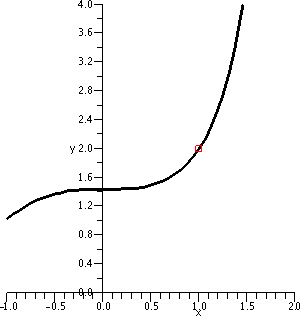 I've forgotten what I did, but I think it was something like:
let's find a solution of y´=x2y which goes through the
point (1,2). So if dy/dx=x2y then dy/y=x2dx and
then ∫dy/y=∫x2dx so that
ln(y)=(1/3)x3+C. If we want this to "go through" (1,2) then
ln(2)=(1/3)13+C so that C=ln(2)–(1/3). And the particular
solution is ln(y)=(1/3)x3+ln(2)–(1/3). Most people,
especially in applications, prefer an explicit solution, so an attempt
to solve for y is made. I can do this here (the situation is simple)
but in general things may be too complicated. The equation
ln(y)=(1/3)x3+ln(2)–(1/3) can be exponentiated to give
y=e(1/3)x3+ln(2)–(1/3). Although for me on an
exam this would be fine, I would not want to mislead you. Again,
especially in applications, appropriate simplification is very
useful. Here this is what would be done:
e(1/3)x3+ln(2)–(1/3)=e(1/3)x3eln(2)e–(1/3)=2e(1/3)[x3–1].
So the particular solution of y´=x2y satisfying the
initial condition y(1)=2 is
f(x)=2e(1/3)[x3–1]. Part of a graph of y=f(x) is
shown to the right. The function increases very quickly when x
is positive.
- Here is an important counterexample:
y´=x2+y2 is a differential equation which
is not separable. This is not totally obvious. Please let me
try to convince you.
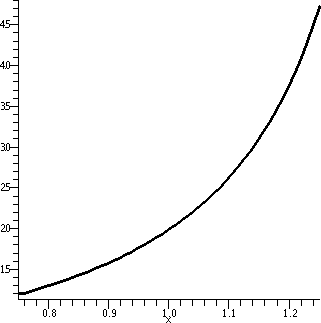
If x2+y2=F(y)G(x) is true, I will "explore" the
possibilities using values of x and y. For example, if x=0 and y=0, we
see that 0=F(0)G(0). Therefore either F(0)=0 or G(0)=0 (or both, of
course). What if G(0)=0? Then try x=0 and y=1. The equation becomes
02+12=F(1)G(0), and this is 1=F(1)G(0). If
G(0)=0, this is impossible! If the alternative holds, that is, F(0)=0, just insert x=1 and y=0 to get a contradiction.
To the right is a picture of the solution curve to
y´=x2+y2 which goes through (1,2). The
function defining the curve can't be written in terms of the standard
functions you know. Quite a bit of computation is needed to produce
the rather simple-looking picture (the darn picture needs a dozen Bessel
functions combined in very strange ways).
Back to the salt tank ...
The differential equation dS/dt=5–[1/(16)]S is
separable. Maybe this is not totally obvious. Look:
5–[1/(16)]S=(5–[1/(16)]S)(1), and 5–[1/(16)]S is a function of S
alone, and 1 is a function of t alone.
Let's separate and solve. So dS/{5–[1/(16)]S}=dt, and the right-hand
side integrates to t+C. The left-hand side is maybe a bit more
intricate. You could substitute: w=5–[1/(16)]S so dw=–[1/(16)]dS and
dS=–16dw. The result is –16ln(w)=–16ln(5–[1/(16)]S). I generally
guess, get it wrong, and need to guess again. So after integrating we have
–16ln(5–[1/(16)]S)=t+C.
The initial condition here, a result of the tank originally being filled with pure water, is S(0)=0. So we can get C:
–16ln(5–[1/(16)]S)=t+C become –16ln(5–[1/(16)]0)=0+C and C is
–16ln(5).
The solution is –16ln(5–[1/(16)]S)=t–16ln(5). Most people prefer a
more explicit formulation, so we solve for S as a function of t.
Divide by –16: ln(5–[1/(16)]S)=–[1/(16)]t+ln(5).
Exponentiate: 5–[1/(16)]S=e–[1/(16)]t+ln(5).
Some algebra on the right:
e–[1/(16)]t+ln(5)=e–[1/(16)]teln(5)=5e–[1/(16)]t.
Now get S: 5–[1/(16)]S=5e–[1/(16)]t becomes
–[1/(16)]S=–5+5e–[1/(16)]t which turns into
S=80–80e–[1/(16)]t.
What does the solution look like?
If we believe S(t)=80–80e–[1/(16)]t, let's check the
initial condition:
S(0)=80–80e–[1/(16)]0=80–80·1=0. Good!
How about the long-range asymptotic behavior? That is, what happens
when t gets very large (t→∞)?
If t→∞, then
–[1/(16)]t→–∞,
so e–[1/(16)]t→0. The combination
80–80e–[1/(16)]t must therefore →80, which is what we
expected. Let's see what the S(t) curve looks like. But here, unlike
in class, I will try to explain the final picture.
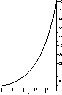
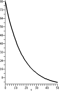
| Here is 80e[1/(16)t for t between –50 and 0. This is
part of an exponential growth curve, and it starts small and increase
up to 80, the value at 0. It is concave up. |
Now I've flipped the curve across the vertical axis. This is
80e–[1/(16)t for t between 0 and 50. The curve is still
concave up, but it is decreasing: since the constant is negative, this is exponential decay. |
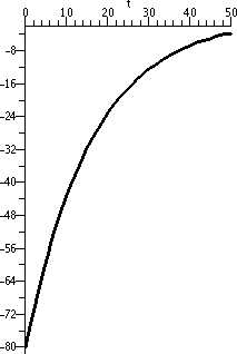
I flipped the previous curve across the horizontal axis. This is a
graph of –80e–[1/(16)t for t between 0 and 50. It is
concave down and increasing, from 80 to near 0. We'll get the real picture of S(t) by translating this up 80.
|
 |
 |
 |
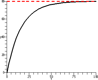
To the right is a graph of S(t)=80–80e–[1/(16)t for t
between 0 and 100. The dashed red horizontal line is at height 80, the
asymptotic level of the salt in the tank. You can see that the salt
starts at 0, the initial condition, and then increases and sort of
curves underneath the line at height 80. The curve is concave
down. The difference between 80 and S(t) becomes rather small as t
grows.
QotD
If we had the time, I would have asked you to find the solution of
y´=y2x3 which goes through (2,1). Be sure
to write the solution as y=some function of x.
| Wednesday,
October 21 | (Lecture #13) |
|---|
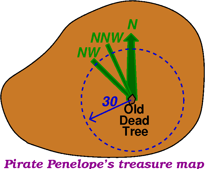 The idea of polar coordinates
You have found a treasure map supposedly giving directions to the
burial spot of a chest full of gold, jewels, mortgages, etc., stolen
by the Dread Pirate Penelope. The information you have is that
A buried treasure is located 30 feet from the
old dead tree, in a
NorthNorthWest direction.
So there you are, on the island. Perhaps the Old dead tree is
still visible. You could mentally draw a circle 30 feet in radius
around the Old Dead Tree. Then you find the North
direction. π/4=45o to the West is NW (Northwest) and
then NNW (Northnorthwest) is π/8 towards North (anyway, you decide
on the direction). Where that direction intersects the circle is
probably where to dig, unless Penelope is tricky, etc.
|
The whole idea of locating a point in a 2-dimensional setting using
distance from a fixed point and angle with respect to a fixed
direction is called polar coordinates.
"Standard issue" polar coordinates
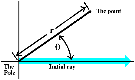
Fix a point (usually called "the center" or sometimes "the pole" and
in most common situations, the origin of the xy-coordinate
system). Also fix a direction -- if needed this might be called "the
initial ray". Almost always this is the positive x-axis in an
xy-coordinate system. Then locate another point in the plane by giving
its distance from the center (called r) and by drawing the line
segment between the center and the point you are locating. Measure the
angle between that and the initial ray (note: counterclockwise is a
positive angle!): this is called θ. Then r and θ
are the polar coordinates of the point.
|  |
An example and the problem with polar coordinates
Well, make the standard choices for "the pole" and "the initial
ray". Let's get polar coordinates (the values of r and θ) for
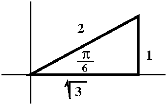
the point whose rectangular coordinates are x=sqrt(3) and y=1. Of
course this is not a random point (sigh). So we consider the picture,
and decide that the hypotenuse (r) should be 2 units long, and the
acute angle (θ) should be π/6. Fine.
But suppose that the point (sqrt(3),1) is operating in a sort of
dynamic way. Maybe it is the end of a robot arm, or something, and
suppose that the arm is swinging around the pole, its angle
increasing. It might be true that we somehow are computing various
angles, and since the arm is moving continuously (still no teleporting
robot arms!) the angles which are θ's should change
continuously. If the arm swings completely around the pole, and comes
back to the same geometric location, it would make more sense to
report its polar coordinates as r=2 and θ=13π/6 (which is
better understood as 2π+π/6).
| 
|
Some valid polar coordinates for the point whose rectangular
coordinates are x=sqrt(3) and y=1:
r=2 and θ=π/6 r=2 and θ=13π/6
r=2 and θ=25π/6 ETC.
But the "robot arm" could also swing around backwards, so other
possible polar coordinates for the same geometric point include
r=2 and θ=–11π/6 r=2 and θ=–23π/6
ETC.
Generally, r=2 and θ=π/6+2π(multiplied by any integer): the integer
could be 0 or positive or negative.
The irritation ("It's not a bug, it's a feature ...") is that there
are further "reasonable" polar coordinate pairs for the same point!
For example, go around to π/6+π. If you position your robot arm
there, and then tell the arm to move backwards 2 units, the arm will
be positioned at (sqrt(3),1). Sigh. So here are some more polar
coordinates for the same point:
r=–2 and θ=7π/6 and
r=–2 and θ=–19π/6
and r=–2 and θ=–31π/6 ETC.
but we are not done yet,
because there are also (going backwards in the angle and the
length)
r=–2 and θ=–5π/6 and
r=–2 and θ=–17π/6 and
r=–2 and θ=–29π/6 ETC.
Generally, r=–2 and θ=7π/6+2π(multiplied by any integer): the integer
could be 0 or positive or negative.
Common restrictions on polar coordinates and the problems they have
This is irritating. Any point in the plane has infinitely many valid
"polar coordinate addresses". In simple applications, people
frequently try to reduce the difficulty. Much of the time, we expect
r>0 always. And maybe we also make θ more calm. The
restriction 0≤θ<2π is used, except when it isn't, so
the restriction –π<θ≤π is used in other
circumstances. I am not trying to be even more incomprehensible than
usual. I am merely reporting what different people do. As we will see,
this is all very nice, except that there are natural circumstances,
both in physical modeling (the robot arm I mentioned and sometimes in
things like understanding the mathematical modeling of big molecules)
and in the mathematical treatment, where it makes sense sometimes to
ignore the artificial restrictions, even if this makes life more
difficult. You'll see a few of these circumstances.
Conversion formulas
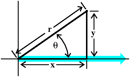 If you consider the picture to the right, I hope that you can fairly
easily "read off" how to go from r and θ to x and y:
x=r cos(θ)
y=r sin(θ)
Going from x and y to r is easy enough:
r=sqrt(x2+y2). If we divide the y equation above
by the x equation, the r's drop out and we get y/x=tan(θ) so
that θ=arctan(y/x). Please note that there are infinitely
many valid r and θ pairs for every point, so this method
will only give you one such pair! Be careful in real applications,
please.
Specifying regions in the plane in polar fashion
It is useful to try to get used to thinking in polar fashion, because
then you will be able to see problems (usually physical or geometric
problems with lots of central symmetry) where this coordinate system
can be used to really simplify computations. So here are some simple
examples of regions which can be easily specified with polar
inequalities.
|
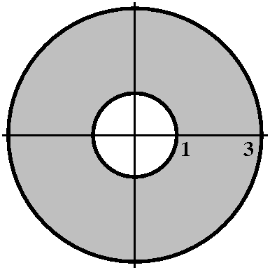
1<r<3
r=1 and r=3 represent two circles centered at 0, one of radius 1 and
one of radius 3. The inequality, which has no restriction on
θ, means that every point between these circles is in the region
specified. This sort of region is frequently called an annulus.
|
|
|
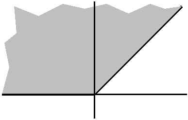
π/4<θ<π
Here there is no restriction on r. I will assume (!!) the standard
restriction that r should not be negative. Then a point is in this
region if its angle with respect to the positive x-axis is more than
π/4 and less than π (the angle π specifies the
negative x-axis!!!). I guess I would call this region a wedge.
I also "guess" that 0 is in this region. The wedge goes out radially
"to infinity" in all of the legal θ directions.
|
|
|
0<r<1 and π/2<θ<5&pi/4
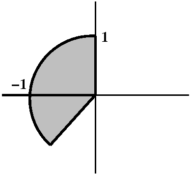
Here are combined restrictions on both polar coordinates. I hope you
can "see" the geometric result. I could describe this region in
rectangular coordinates, certainly, but the needed equations and
inequalities would be much more complicated to me. Maybe this sort of
thing will give you some appreciation of the usefulness of polar
coordinates.
|
|
We will study the equations and graphs of some polar curves next time,
and we will do a bit of calculus (arc length and area). That will
conclude the course lectures.
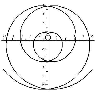
A first polar curve (a weird one!)
We tried to sketch as well as possible all points in the plane which have
r=θ using any (!) determination of polar coordinates (no
restrictions on r and θ). The result is weird until you get used
to it (as usual!).
To the right is Maple's graph of
r=θ when –12≤θ≤12. Think hard about
what the graph would look like for θ small positive (in the
first quadrant) and θ small negative (although the "robot arm"
is pointing in the fourth quadrant, the corresponding r value is
negative, so the curve appears in the second quadrant, near the
negative x-axis). The curve is smooth with no corners or cusps, and
has infinitely many self-intersections on the y-axis.
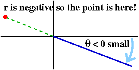
Most people understand the θ>0 part of the curve but the part
with θ<0 was more difficult, because we must remember
to go backwards when r is negative (this happens because the
curve is r=θ). The picture shown is something which might help
people to understand.
I don't think negative r's will occur very often in practice (but they
do -- see a few of the curves below). This curve is an example
of an Archimedean
spiral (although usually r>0 in the description of that
spiral).
Today I'll do some calculus in polar coordinates with the object being
(as I mentioned in class) to get two formulas which you are supposed
to know. I'll first sketch some "classical" polar coordinate curves,
and then I'll do some computations with arc length and area. Here are
some examples with numbers maybe a bit nicer than what was done in
class.
A collection of examples
r=3+sin(θ)
Let's consider r=3+sin(θ). Since the values of sine are all
between –1 and 1, r will be between 2 and 4. Any points on this curve
will have distance to the origin between 2 and 4 (the green and red
circles on the accompanying graph). When θ=0 (the positive
x-axis)
r is 3. As θ
increases in a counterclockwise fashion, the value of r increases to 4
in the first quadrant. In the second quadrant, r decreases from 4 to
3. In the third quadrant, corresponding the sine's behavior (decrease
from 0 to –1) r decreases from 3 to 2. In all of this {in|de}crease
discussion, the geometric effect is that the distance to the origin
changes. We're in a situation where the central orientation is what
matters, not up or down or left or right. Finally, in the fourth
quadrant r increases from 2 to 3, and since sine is periodic with
period 2Π, the curve joins its earlier points.
The picture to the right shows the curve in black. I'd describe the
curve as a slightly flattened circle. The flattening is barely
apparent to the eye, but if you examine the numbers, the up/down
diameter of the curve is 6, and the left/right diameter is 6.4.
| 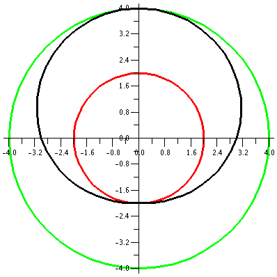
|
Converting to rectangular coordinates
A naive person might think, "Well, I could convert the equation
r=3+sin(θ) to rectangular coordinates and maybe understand it
better." Except under rare circumstances (I'll show you one below),
the converted equation is very irritating and difficult to
understand. For example, Let's start with r=3+sin(θ) and
multiply by r. The result is r2=3r+r·sin(θ). I
multiplied by r so that I would get some stuff I'd recognize from the
polar/rectangular conversion equations. r2 is
x2+y2 and r·sin(θ) is y. So I have
x2+y2=3r+y, or
x2+y2–y=3r. I would rather avoid square roots so
I will square this, and get
(x2+y2–y)2=9r2=9(x2+y2).
This is a polynomial equation in x and y of highest degree 4, defining
this curve implicitly. The equation doesn't give me much
insight.
|
r=2+sin(θ)
Now consider r=2+sin(θ). Again,
the values of sine are all between –1 and 1, so r will be between 1
and 3. Any points on this curve will have distance to the origin
between 1 and 3. We can begin (?) the curve at θ=0 when r=2, and spin around
counterclockwise. The distance to the origin increases to r=3 at θ=Π/2 (the positive y-axis). The
distance to the origin decreases back to r=2 when θ=Π (the negative x-axis). The
curve gets closest to the origin when θ=3Π/2 (the negative y-axis) when r=1. Finally, r increases
(as θ increases in the
counterclockwise fashion) to r=3 again when θ=2Π.
Here the "deviation" from circularity in the curve is certainly
visible. The bottom seems especially dented.
| 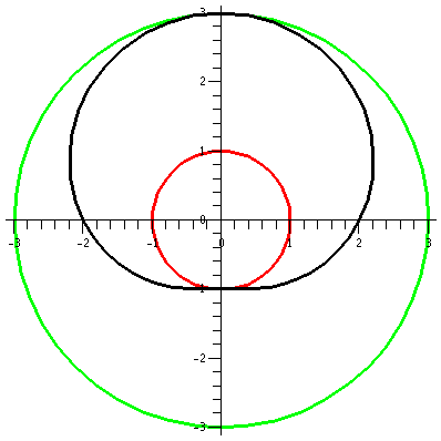
|
r=1+sin(θ)
We decrease the constant a bit more, and look at r=1+sin(θ). The values of sine are all
between –1 and 1, so r will be between 0 and 2. The (red) inner circle
has shrunk to a point. This curve will be inside a circle of radius 2
centered at the origin. We begin our sweep of the curve at 0, when r
is 1. Then r increases to 2, and the curve goes through the point
(0,2). In the θ interval from
Π/2 to Π, sin(θ) decreases
from 1 to 0, and the curves moves closer to the origin as r decreases
from 2 to 1. Something rather interesting now happens as θ travels from Π to 3Π/2 and then
from 3Π/2 to 2Π.  The rectangular graph of 1+sine, shown here, decreases
down to 0 and then increases to +1. The polar graph dips to 0 and then
goes back up to 1. The dip to 0 in polar form is geometrically a sharp
point! I used "!" here because I don't believe this behavior is easily
anticipated. The technical name for the behavior when r=3Π/2 is
cusp. The rectangular graph of 1+sine, shown here, decreases
down to 0 and then increases to +1. The polar graph dips to 0 and then
goes back up to 1. The dip to 0 in polar form is geometrically a sharp
point! I used "!" here because I don't believe this behavior is easily
anticipated. The technical name for the behavior when r=3Π/2 is
cusp.
This curve is called a cardioid from the Latin for "heart"
because if it is turned upside down, and if you squint a bit, maybe it
sort of looks like the symbolic representation of a heart. Maybe.
| 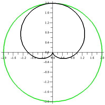
|
r=1/2+sin(θ)
Let's consider r=1/2+sin(θ). The values of sine are all
between –1 and 1, so r will be between –1/2 and 3/2. The (red) inner
circle actually had "radius" –1/2, and it consists, of course, of
points whose distance to the pole, (0,0), is 1/2. When θ is 0, r is 1/2. In the first two
quadrants, 1/2+sin(θ) increases
from 1/2 to 3/2 and then backs down to 1/2. In the second two
quadrants, when θ is between Π
and 2Π, more interesting things happen.
 The rectangular graph on the interval [0,2Π] of sine moved up by 1/2
shows that this function is 0 at two values, and is negative between
two values. The values are where 1/2+sin(θ)=0 or sin(θ)=–1/2. The values of θ satisfying that equation in the
interval of interest are Π+Π/6 and 2Π–Π/6. The curves goes down to
0 distance from the origin at Π+Π/6, and then r is negative until
2Π–Π/6. The natural continuation of the curve does allow negative
r's, and the curve moves "behind" the pole, making a little loop
inside the big loop. Finally, at 2Π–Π/6, the values of r become
positive, and the curve links up to the start of the big loop.
This curve is called a limaçon ( got thing wrong in class
-- I'm sorry). The blue lines are lines with
θ=Π+Π/2 and θ=2Π–Π/6. These lines, for the θ
values which cross the pole, are actually tangent to the curve at the
crossing points.
| 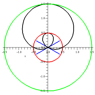
|
r=0+sin(θ)
Let's try a last curve in this family, with the constant equal to
0. What does r=sin(θ) look like? A graph is shown to the right.
There are several interesting features of this graph. First, this is a
polar curve which does have a nice rectangular (xy) description. If we
multiply r=sin(θ) by r, we get
r2=r·sin(θ), so that
x2+y2=y. This is x2+y2–y=0
or, completing the square,
x2+y2–2(1/2)y+(1/2)2–(1/2)2=0
so that (x–0)2+(y–1/2)2=(1/2)2. This
is a circle of radius 1/2 and center (0,1/2), exactly as it looks.
The moving "picture" of this curve is quite different. Between
0 and π it spins once around the circle but then from π to 2π
it goes around the circle another time! So this is really somehow two
circles, even though it looks like only one geometrically. This is
hard to understand.
| 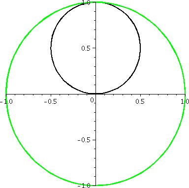
|
More information about these curves is available here.
Area of polar curves
The area of the region enclosed by the rays r=α and r=β and the polar
curve r=r(θ) (r is some function of θ) is the (initially)
silly-looking integral
{1/2}∫θ=αθ=β(r(θ))2dθ.
I tried to motivate this formula by considering areas of circular
sections of radius R and central angle ψ. After considering
examples, we first "guessed" that the area would be directly
proportional to R2 and that the constant of proportionality
was ψ/2 (this only works so easily if we use radian measure
for angles). This observation can then be applied to find the area of
the region by slicing the region using many narrowly placed "rays"
coming from the origin so that we had regions with central angle
dθ and radius r(θ). This is discussed in the textbook on
p. 649. I mentioned that we could apply this to find the area inside a
limaçon.
Length of polar curves
The formula is
∫θ=αθ=βsqrt(r2+(dr/dθ)2)dθ. This formula is gotten from the parametric
curve formula on p.652 of the textbook. Please look at the examples in
the textbook.
There is no class time for more examples of polar curves next time but
what follows may be useful.
"Sketching" roses
Here are dynamic pictures of two roses. The first is
r=cos(3θ). It is "covered" or traced twice and has 3
"petals". The second is r=cos(4θ). It is only covered once, and
it has 8 petals! Wow, polar coordinates can be annoying!
| | |
r=cos(3 )
This is a three-leafed rose. Please note that the graph shows one
sweep, as θ goes from 0 to 2Π. )
This is a three-leafed rose. Please note that the graph shows one
sweep, as θ goes from 0 to 2Π.  The rectangular graph, shown here, has three pairs of ups
and downs. The polar trace covers the leaves twice. The six
up-and-downs of cos(3θ) (magically?) reduce to retracings of
half of the loops. I hope I made this evident. I
introduced some deliberate distortion in the second
tracing. (!) Without the distortion, the second tracing
could not be seen at all. The imaginary "point" travels over the
computer screen's pixels and colors them (from white to black in this
case). The second trip could not be noticed since the pixels had
already been flipped to black. So I put in a small perturbation so
that the second layer of travel could be seen. The rectangular graph, shown here, has three pairs of ups
and downs. The polar trace covers the leaves twice. The six
up-and-downs of cos(3θ) (magically?) reduce to retracings of
half of the loops. I hope I made this evident. I
introduced some deliberate distortion in the second
tracing. (!) Without the distortion, the second tracing
could not be seen at all. The imaginary "point" travels over the
computer screen's pixels and colors them (from white to black in this
case). The second trip could not be noticed since the pixels had
already been flipped to black. So I put in a small perturbation so
that the second layer of travel could be seen.
| 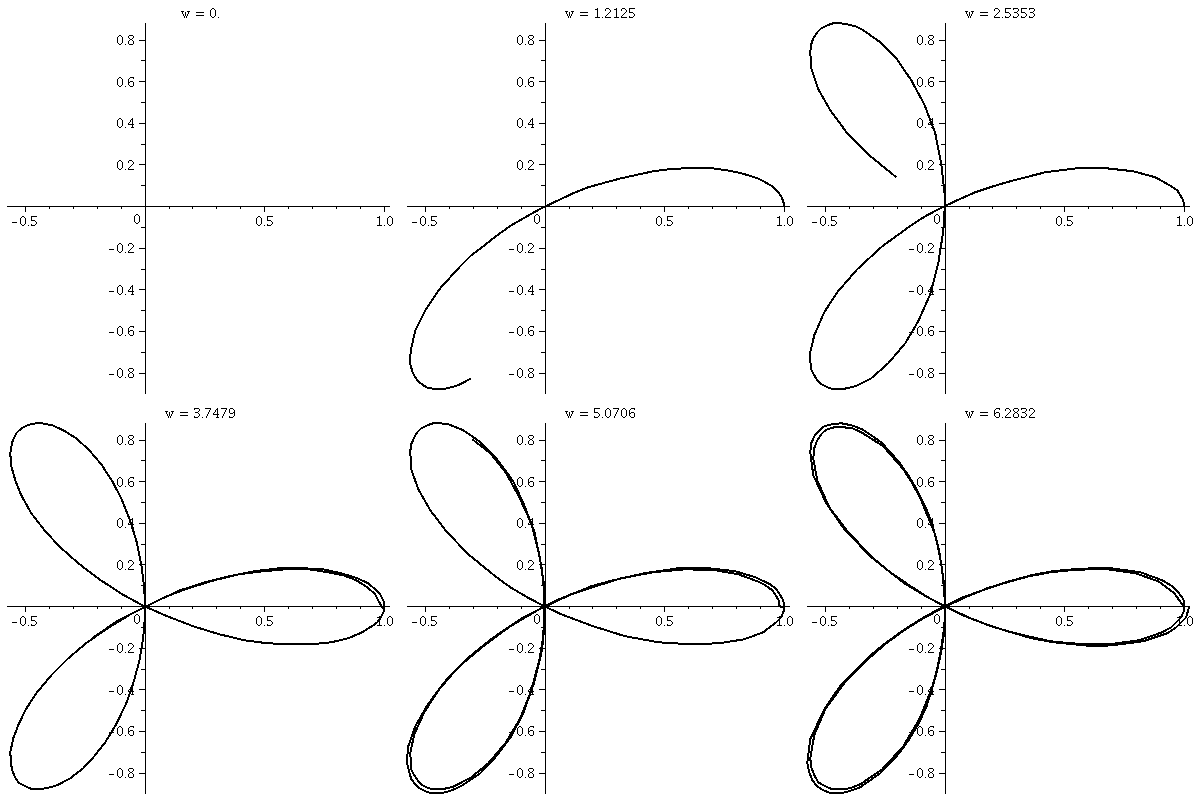
|
| | |
r=cos(4θ)
This "rose" has 8 leaves or petals, and
the dynamic way it is traced is weird and wonderful to me.  The rectangular
graph. to the right, shows four bumps up and four bumps down. There
are no retracings of already colored points, so that the wiggles up
and down of cos(4θ) all result in 8 leaves. The rectangular
graph. to the right, shows four bumps up and four bumps down. There
are no retracings of already colored points, so that the wiggles up
and down of cos(4θ) all result in 8 leaves.
| 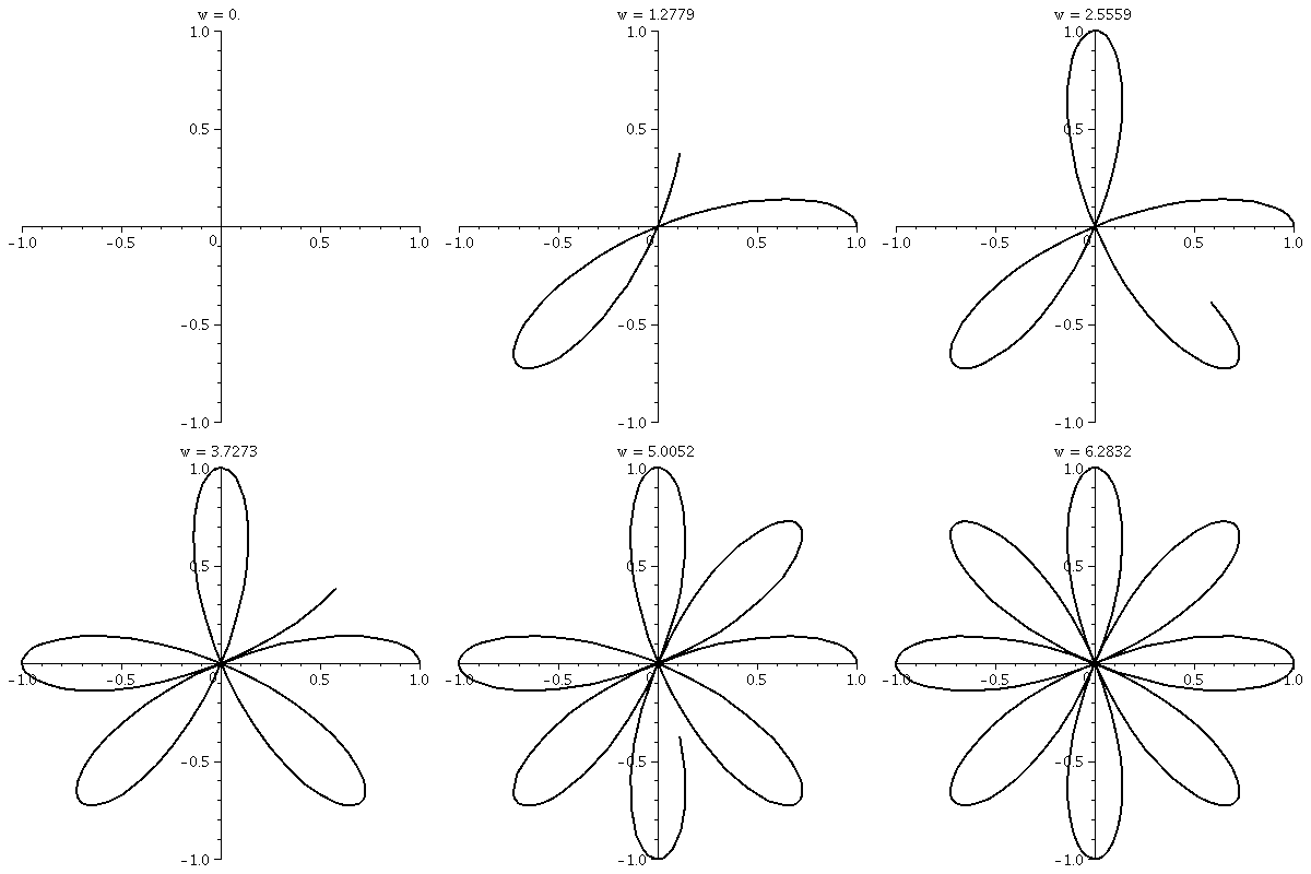
|
| | |
Area inside one petal of r=cos(3θ)
Well, cos(3θ) "first" (going from 0 to 2π) is 0 when
3θ=π/2. So we get half a petal by integrating from 0 to
π/6. The formula is
∫αβ(1/2)r2dθ for
area in polar coordinates (see the discussion on p.649 of the
textbook), so this becomes (for the whole petal, we need to
double):
2·(1/2)∫0π/6
cos(3θ)2dθ. This can be computed using a trig
identity.
| 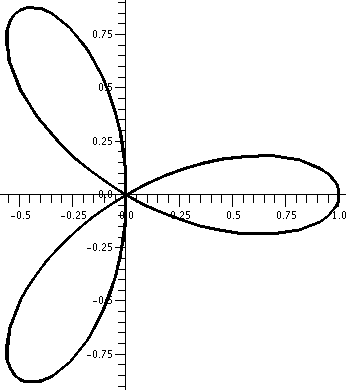 |
| | |
Another kind of spiral
I didn't talk about Exponentials and snails, darn it! Curves
of the form r=a ebθ are spirals of a different
kind than what we've drawn (for example, different from the spiral
drawn for the QotD last time). All of these spirals have a strange and
wonderful geometric property. If a ray is drawn from the pole (the
origin) then the angle the ray makes with the tangent line of the
spiral at any intersection is the same. I attempted to
illustrate this with the first picture to the right. It turns out that
this silly geometric property has natural consequences in terms of the
energy efficiency of its construction. A snail shell when considered
transversal (perpendicular) to the axis of symmetry usually is one of
these curves and different species has different constants, b. You
can read a
wikipedia article about these spirals, which have a number of
different names (of course!).
To the right is a machine-drawn picture of r=e.25θ
as θ goes from
–Π to 5Π. The .25 was put in to make the exponential not
grow too fast so the picture would be tolerable.
|
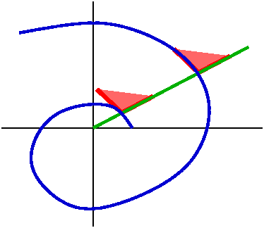
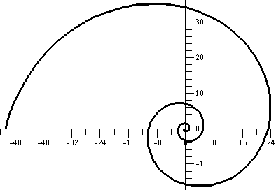
|
|
| Monday,
October 19 | (Lecture #12) |
|---|
A bug drawing out a thread ...
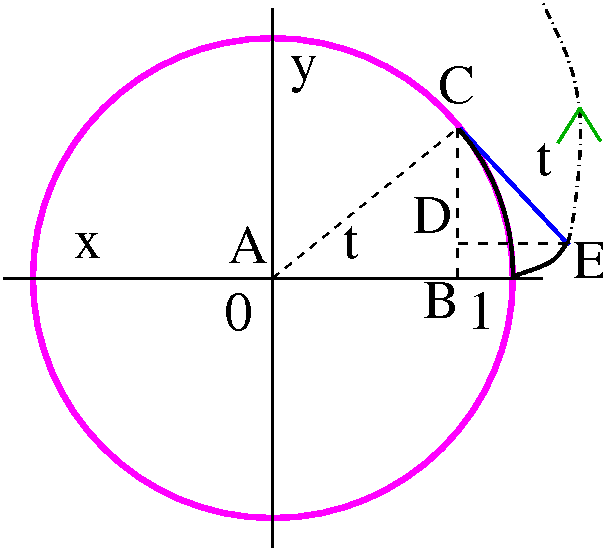 Thread is wound around the unit circle centered at the
origin. A bug starts at (1,0) and is attached to an end of the
thread. The bug attempts to "escape" from the circle traveling
counterclockwise. The bug moves at unit speed.
I would like to find an expression for the coordinates of the bug at
time t. Look at the diagram. The triangle ABC is a right triangle, and
the acute angle at the origin has radian measure t. The hypotenuse
has length 1, and therefore the "legs" are cos(t) (horizontal leg, AB)
and sin(t) (vertical leg, BC). Since the line segment CE is the bug
pulling away (!) from the circle, the line segment CE is tangent to
the circle at C. But lines tangent to a circle are perpendicular to
radial lines. So the angle ECA is a right angle. That means the angle
ECD also has radian measure t. But the hypotenuse of the triangle ECD
has length t (yes, t appears as both angle measure and length
measure!) so that the length of DE is t sin(t) and the length of
CD is t cos(t).
The coordinates of E can be gotten from the coordinates of C and the
lengths of CD and DE. The x-coordinates add (look at the picture) and
the y-coordinates are subtracted (look at the picture). Therefore the
bug's path is given by x(t)=cos(t)+t sin(t) and
y(t)=sin(t)–t cos(t).
Radian measure is used in several ways here. The angle BAC is the same
as the arc length from (1,0) to C along the circle and this is the
same as the length of the line segment EC.
| t between 0 and 1 | t between 0 and 10
Note that the scale is changed! |
|---|
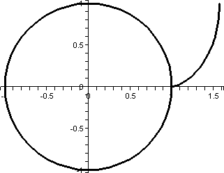 |
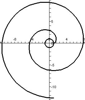 |
Finally to the right is an animated picture of the bug moving. Maybe
you can understand this picture better: maybe (!!).
This curve is more typical of parametric curves. I don't know any easy
way to "eliminate" mention of the parameter. This seems to be an
authentically (!) complicated parametric curve, similar to many curves
which arise in physical and geometric problems. It has an official
name. It is called the evolute of the circle.
| 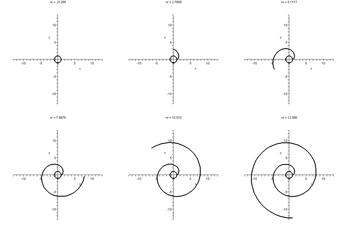
|
Parametric curves
We begin our rather abbreviated study of parametric curves. These
curves are a clever way of displaying a great deal of
information. Here both x and y are functions of a parameter. The
parameter in your text is almost always called t. The simplest
physical interpretation is that the equations describe the location of
a point at time t, and therefore the equations describe the motion of
a point as time changes. I hope examples will make this more
clear. The t here is usually described for beginners as time, but in
applications things can get a great deal more complicated. Parametric
curves could be used to display lots of information. For example, some
steels contain chromium. Maybe the properties of the steel such as
ductility (a real word: "The ability to permit change of shape without
fracture.") and density, might depend on the percentage of
chromium. So the t could be that and the x and y could be measurements
of some physical properties of the steel. Here x=f(t) and y=g(t), as
in the text. Now a series of examples.
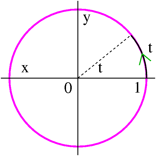 Example 1
Suppose x(t)=cos(t) and y(t)=sin(t). I hope that you recognize almost
immediately that x and y must satisfy the equation
x2+y2=1, the standard unit circle, radius 1,
center (0,0). But that's not all the information in the equations.
The point (x(t),y(t)) is on the unit circle. At "time t" (when the
parameter is that specific value) the point has traveled a length of t
on the unit circle's curve. The t value is also equal to the radian
angular measurement of the arc. This is uniform circular
motion. The point, as t goes from –∞ to +∞, travels
endlessly around the circle, at unit speed, in a positive,
counterclockwise direction.
Example 2
Here is a sequence of (looks easy!) examples which I hope showed
students that there is important dynamic (kinetic?) information in the
parametric curve equations which should not be ignored.
- x(t)=t and y(t)=t. Surely the "particle" travels on the main
diagonal line y=x. The travel (remember, the domain unless otherwise
limited, is all values of t which makes sense to the defining
functions) is from lower left (third quadrant) to upper right, (first
quadrant). Also I hope that you see the particle moves at uniform
speed. This is uniform linear motion.
| 
|
- x(t)=t3 and y(t)=t3. The path of this point
is also on the main diagonal line y=x. But the motion of this point,
while in the same direction as the first example (from third to first
quadrant), is very different. The difference is in the "clock". Try a
few values of t. Between t=0 and t=1 we travel from (0,0) to
(1,1). Between t=1 and t=2, we travel from (1,1) to (8,8). Just
roughly, the distance changes from sqrt(2) to sqrt(98). That's a big
change. The particle, near –∞, travels fast. Then as t goes
around 0, it is slower, and, as t gets very large positive, the
particle moves faster.
| 
|
- Now let's consider the motion described by x(t)=t2 and
y(t)=t2. Again, we can "eliminate the parameter". That
rather grim phrase (if you read murder mysteries!) is what the text
uses to describe getting rid of t by manipulating the two
equations. Here we just realize that x=y. Much of the information
about the motion of this point on the main diagonal is lost if we go
to just y=x. The t2 means that both x and y must be
non-negative. When t is large negative, the point is way up high in
the first quadrant, and traveling towards the origin rather
rapidly. It begins to slow, and then "stops" (!) but only
"instantaneously" (!!) at (0,0) (when t=0). It turns around (how the
heck does a particle "turn around"?) and begins to retrace its path,
up towards the open end (??) of the first quadrant. As it travels, its
speed increases. So this is really quite complicated motion, and very different from the first two examples.
| 
|
- The final example in this series is x(t)=cos(t), and
y(t)=cos(t). Again, the path traveled by the point is on the main
diagonal line y=x. But now the dynoamics are extremely
different. Because cosine oscillates endlessly between –1 and +1, the
motion of the point whose position is described by these equations is
on the line y=x and only between (–1,–1) and (1,1). It moves back and
forth between these points, completing a round trip in every time interval of length 2Pi. This is very different motion from the other examples.
| 
|
Example 3
I considered x(t)=5cos(t)and y(t)=5sin(t). This is a slight
variant of the very first example. Since x(t)/5=cos(t) and
y(t)/5=sin(t), I "know" that the particle's path must be on
(x/5)2+(y/5)2=1, so
x2+y2=52, a circle whose center is
(0,0) and radius is 5.
The fact that the path lies on the circle whose equation is given is
fairly clear. But I was asked a slightly different question in class:
why does the point travel in a counterclockwise direction? When
you learn about velocity vectors, this may also be "fairly" clear, but
right now, if you plug in t=0, the point (x(t),y(t)) is (5,0), and if
you plug in π/2, the point is (0,5). Therefore I feel that travel
proceeds in a counterclockwise direction, from (5,0) to (0,5) and so
on.
|

|
What if x(t)=5cos(t) and y(t)=3sin(t)? Then the
trig identity gives (after elimination of the parameter)
(x/5)2+(y/3)2=1 as the possible path of the
point. This is an ellipse centered at (0,0). Its wider part (total
length 10) is on the horizontal axis, as shown. The vertical extant of
the ellipse is 6.
So I attempted to create a moving image of this curve. I hope it is
helpful to you. The parameterization is by central angle. Speed
varies. (I will discuss this more below.)
| 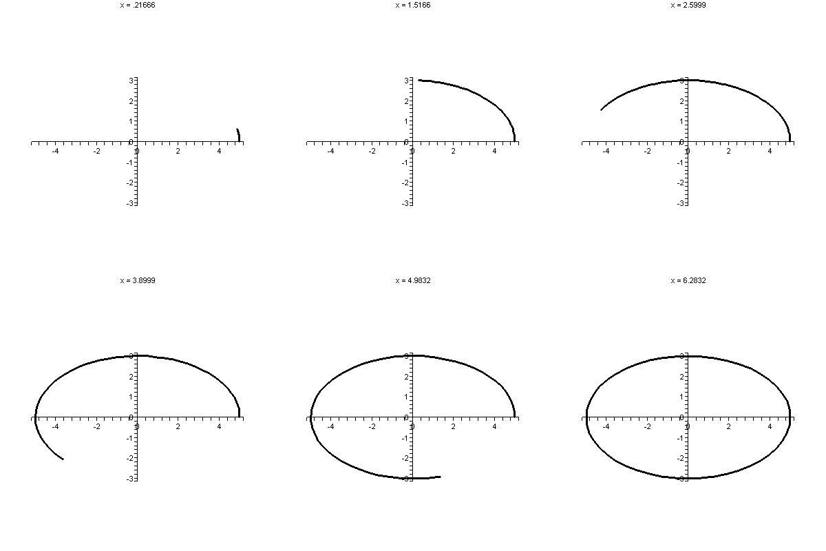
|
My favorite parametric curve
This is x(t)=1/(1+t2) and y(t)=t3–t. I
would like to analyze this curve a bit differently from the other
examples by separately considering the horizontal and vertical
components.
| The horizontal control |
|---|
|
Here we consider x as a function of t. The function has even degree
and is therefore symmetric: if (t,x) is on the curve, so it
(–t,x). Actually, the function is relatively simple. Consider positive
t. As t increases, x decreases, and since 1+t2→∞
x→0. So we get a picture as shown below.
Since this represents the horizontal part of the motion described by
this parametric curve, the result is this in the (x,y) plane: the
point for large negative t starts close to the x-axis. Then as t
increases, it slowly moves right. At its largest it is 1 unit to the
right of the vertical axis. Then it slowly moves back towards the
vertical axis again.

|
| The vertical control |
|---|
|
In this case, I'm considering the y-component of the moving point. I
could think of this as the vertical control of some sort of scanning
machine. The function has odd degree and is antisymmetric (if (t,y) is
on the curve, then (–t,–y) is on the curve). It is a cubic polynomial
with three real roots, at 1, –1, and 0. The graph is shown to the
right.
The curve in the (t,y) plane starts very low left, then up, then down,
then up, way way up on the right.
But this is a description of the vertical motion. Now what could we
"see" in the (x,y) plane? The point
starts way way down (this is large negative y!), moves up,
bounces down, and then finally moves way way up.
|  |
|
 Combining these two motions can be difficult to do but with practice
you will find it easier. A part of the combined motion, the whole
parametric curve, is shown to the right. Indeed, it is a curve with a
self-intersection.
I don't know how to describe this curve accurately and efficiently
without the parametric "apparatus". The self-intersection occurs when
t=1 and t=–1 (that's where x=0 and y<1, as shown in the
picture). The point at which this occurs is (0,1/2).
|
Calculus?
Finally, very late in the lecture, I attempted some calculus. Here's
what I said.
Suppose we want to analyze what happens when the parameter changes
just a little bit, from t to t+Δt. Well, the point starts at
(f(t),g(t)). What can we say happens at t+Δt? Well,
f(t+Δt)≈f(t)+f´(t)Δt. Why is this true? You can
think of this either 151 style (calc 1) as linear approximation, or
you will see a more sophisticated 152 approach in a few weeks.
Similarly for g(t) we know
g(t+Δt)≈g(t)+g´(t)Δt. Therefore the point in
the interval [t,t+Δt] moves from (f(t),g(t)) to (approximately!)
(f(t)+f´(t)Δt,g(t)+g´(t)Δt). What is the slope
of the line segment connecting these points?
Slope
Take the difference in second coordinates divided by the difference in
the first coordinates. The result (there is a lot of cancellation) is
g´(t)/f´(t). If this were an xy curve, this would be noted
as dy/dx, the slope of the tangent line. In fact, people usually
remember the result in the following way:
dy   dy/dt
-- = -----
dx   dx/dt
and this can be used to get tangent lines.
A tangent line to the evolute
Let me find a tangent line to the evolute of a circle when t=3Π/4.
For this, x(t)=cos(t)+t sin(t) and
y(t)=sin(t)–t cos(t). When t=3Π/4,
x=–[1/sqrt(2)]+3Π/sqrt(2) (approximately 0.95897) and
y=[1/sqrt(2)]+3Π/sqrt(2) (approximately 2.37319). So we know a
point the line goes through. How about the slope?
dy/dx=(dy/dt)/(dx/dt)=[cos(t)–cos(t)+t sin(t)]/[–sin(t)+sin(t)+t cos(t)]=tan(t)
(amazing that it is so relatively simple). At t=3Π/4, this is
–1. So the line is
y–[1/sqrt(2)]+3Π/sqrt(2)=(–1)(x–{–[1/sqrt(2)]+3Π/sqrt(2)}). The
line and the curve are shown to the right.
| 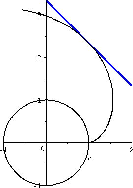 |
Speed
Since Distance=Rate·Time, and in the time
interval [t,t+Δt] we move from (f(t),g(t)) to (approximately!)
(f(t)+f´(t)Δt,g(t)+g´(t)Δt), we can get the speed
(the Rate) by taking the distance between these points and dividing by
Δt. There is more cancellation here, and the result is
Speed=sqrt(f´(t)2+g´(t)2) or
         ___________
        /(dx)2 (dy)2
Speed= / (--)+ (--)
      /  (dt)  (dt)
As you'll see if you take Math 251,
this is the sum of the squares of the
horizontal and vertical components of the velocity vector: it is,
in fact, the magnitude of the velocity vector.
Length of a curve
Well, suppose we move along a parametric curve given by x=f(t) and
y=g(t) from t=START to t=END. If we believe that the
speed is sqrt(f´(t)2+g´(t)2), then we
know that this speed can vary. In a short time interval (a time
interval which is dt long!) the
distance traveled is Speed·Time, or
sqrt(f´(t)2+g´(t)2)dt. We can add up
all these distances from t=START to t=END using the
integral idea. So the distance traveled along the curve from
t=START to t=END will be given by
∫t=STARTt=ENDsqrt(f´(t)2+g´(t)2)dt.
(We are integrating the magnitude of the velocity vector). Is this a
reasonable formula?
Almost no speed functions have nice, neat, simple antiderivatives. In
the real world, you'll need to use numerical approximation. However,
Math 152 is not the real world.
A textbook problem
Section 11.3, problems 3 through 15, are all "Find the length of the
path over the given interval" with some rather silly-looking functions
specified. Accidentally (exactly not accidentally, actually!)
all of the problems can be computed exactly with antiderivatives and
values of standard functions. There is a fair amount of ingenuity
involved in constructing such examples. I urged students to practice
with several of them. Here is problem #7:
Find the length of the path described by
(3t2,4t3), 1≤t≤4.
The solution
Here x=3t2 and y=4t3. We will compute the speed
and then attempt to "integrate" (actually using FTC, so we'll need to
find the antiderivative). Now dx/dt=6t and
dy/dt=12t2. Therefore the speed is sqrt(6t)2+(12t2)2). This is
sqrt(36t2+144t4). We'll need to integrate this,
and maybe I will "simplify" first. Indeed, since we consider t in an
interval where t≥0, sqrt(t2)=t (otherwise we would need
to worry about |t| or –t etc.). But
36t2+144t4=36t2(1+4t2) so
that the square root is 6t·sqrt(1+4t2). Therefore
the distance traveled along the curve is an integral,
∫t=1t=46t·sqrt(1+4t2)dt.
Several students immediately suggested various substitutions. Here is
one which does the job efficiently. So:
If u=1+4t2, du=8t dt, so (1/8)du=dt.
∫6t·sqrt(1+4t2)dt=(6/8)∫sqrt(u)du.
Now
(6/8)∫sqrt(u)du=(6/8)(2/3)u3/2+C=(1/2)u+C=(1/2)(1+4t2)3/2+C.
So
∫t=1t=46t·sqrt(1+4t2)dt=(1/2)(1+4t2)3/2|14=(1/2)(65)3/2–(1/2)(5)3/2.
 Tangent lines
I'll find the tangent lines at the self-intersection point of my favorite curve. The point involved is (1/2,0) and
the two values of t are +1 and –1. Since I have the point, the other
information I need to find the tangent lines is the slope. Well, slope
is dy/dx=(dy/dt)/(dx/dt).
Since x=1/(1+t2),
dx/dt=(–2t)/(1+t2)2. I only fouled this up two
or three times in class, but when t=–1, dx/dt=1/2, and when t=+1,
dx/dt=–1/2.
Since y=t3–t, dy/dt=3t2–1. When t=–1 or when
t=+1, dy/dt=3–1=2.
Therefore when t=–1, dy/dx=(2)/(1/2)=4. The line goes through (1/2,0),
so an equation for it is y=4(x–1/2).
Therefore when t=1, dy/dx=(2)/(–1/2)=–4. The line goes through (1/2,0),
so an equation for it is y=–4(x–1/2).
I had Maple graph the parametric curve
and the two lines just found (in green and
blue). I then asked what the angle between the
lines (the angle which encloses the x-axis). The angle is 151.9
degrees. Hey, please remember that the slope of a line is the tangent
of the angle that the line makes with the positive x-axis. Here the
angle between the
line y=4(x–1/2) and the positive x-axis has angle equal to arctan(4),
approximately 1.326 radians. Double this is about 151.9 degrees. Hey:
we have the machines. Please use them.
Uniform speed?
We developed a formula for speed. It was
sqrt(f´(t)2+g´(t)2) where x=f(t) and
y=g(t). For the circle x=5cos(t) and y=5sin(t), previously considered, we know dx/dt=–5sin(t) and
dy/dt=5cos(t), so that (dx/dt)2+(dy/dt)2=25((sin(t))2+(cos(t))2)=25·1=25, so the speed, which is the square
root, is always 5. So this is uniform circular motion: the word
"uniform" here means that the speed is constant. (Notice, oh physics
people, that I am not saying the velocity is constant and I am not
saying that the acceleration is 0. Indeed, both of those statements
are false. The direction of the velocity is changing, so the
acceleration is not 0. We need to look at these quantities as
vectors, and this will be done in Math 251.)
Nonuniform speed
Then I tried to analyze an ellipse we had parameterized
earlier. We have x(t)=5cos(t) and y(t)=3sin(t) so
dx/dt=–5sin(t) and dy/dt=3cos(t), and the speed is the square
root of 25(sin(t))2+9(cos(t))2=
16(sin(t))2+9(sin(t))2+9(cos(t))2=
16(sin(t))2+9 since sin2+cos2 is
1. Sigh. The speed at time t is sqrt(16(sin(t))2+9). When
t=0, the particle whose motion we are describing is at (5,0) and the
speed is sqrt(9)=3 since sin(0)=0. When t=Π/2, the particle is at
(0,3) and the speed is sqrt(25)=5 since sin(&pi/2)=1. So certainly the
particle is not moving at the same speed. Indeed, a graph of the
speed, sqrt(16(sin(t))2+9), is shown to the right.
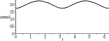 Now this does resemble what I know about the motion of a planet in
orbit. When it is far away from the center of the orbit, the planet
will have large potential energy and relatively small kinetic energy
(it will move slowly). This is near t=0 and t=Π. When it is close
to the center of the orbit, the planet moves faster, and the kinetic
energy is larger, while the potential energy, measured by the work
needed to move closer/farther from the center, decreases.
The total energy is conserved, but the way the total is divided
between kinetic and potential energy varies. Maybe if you look
again at the moving picture, you will "see" both of these
phenomena. They are not too clear to me visually.
Back to my favorite curve
The length of the loop in my favorite curve can be gotten by computing
the integral of the speed from –1 to +1 (the two self-intersection
times). So this is (I'll use the formulas we already have)
∫–11sqrt((–2t/(1+t2)2)2+(3t2–1)2)dt.
Maple takes more than half a second
(quite a lot of time!) to acknowledge that it can't find an
antiderivative, so we can't use FTC. In less than a tenth of a second,
the approximate value 1.971944073 is reported.
|
| Wednesday,
October 14 | (Lecture #11) |
|---|
Two silly (?) formulas
The object of this lecture is to tell you about two formulas, one for
arc length and one for surface area (both discussed in section 8.1). I
called the formulas silly because of their limited usefulness, at
least limited in the sense that "hand computation" using FTC is not
very practical. Arc length and surface area will be addressed again in
calc 3, where much better perspectives can be given for both.
The philosophy behind the definite integral and its use
Maybe the formulas are not totally silly. Both of them are
illustrations of how definite integrals can be used to compute various
quantities. The procedure (which we have already used in various area
and volume situations, and also with work) represents an attempt to
compute "something" complicated:
- Break up the complicated quantity into little pieces.
- Approximate the little pieces by something simple.
- Add up the little pieces, and take a limit.
With some luck and skill and ... whatever, the errors which occur will
be small, and as the number of subdivisions or pieces or whatever
grow, the total error will get small.
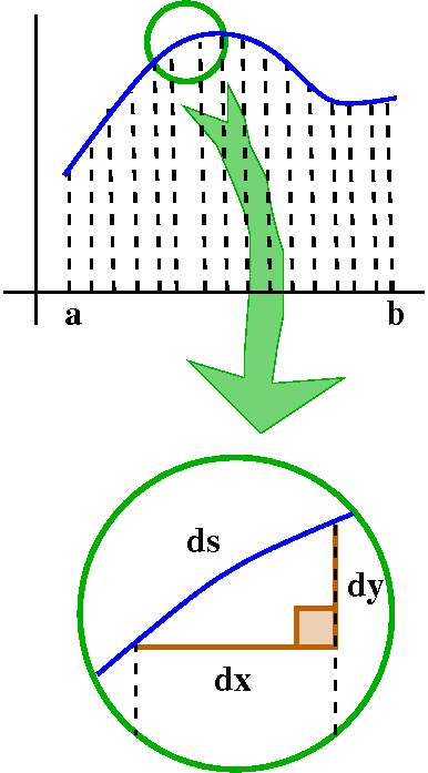 Arc length
We're given a function, f(x), defined on the interval [a,b].
The quantity to be computed is the length of the graph, the curve
y=f(x). This is called arc length. Here is the idea.
Break up [a,b] into many little subintervals, whose length we will
call dx (or Δx). "Above" each little subinterval is a little
piece of the curve. The usual name for a little piece of curve is
ds. If you magnify the little piece, as shown, well, the result is
almost a right triangle. The curve length is still somewhat curvy,
but, well, maybe I can approximate it by a straight line segment. The
resulting picture is just about a right triangle. dy is the change in
y (the function) when the input variable, x, Pythagoras then
declares that (ds)2 should be the same (really,
approximately the same!) as
(dx)2+(dy)2. Therefore
ds=sqrt{(dx)2+(dy)2). Let's rewrite what's
inside the square root:
(dx)2+(dy)2=(dx)2(1+{dy/dx}2).
So sqrt(=(dx)2(1+{dy/dx}2))=dx·sqrt(1+{f´(x)}2).
("Factoring out" the dx is strange to me, and so is recognizing the
quotient dy/dx as the derivative.)
Now we should add up these pieces and take limits. In this context,
this is all done by writing a definite integral. So the arc length
formula is ∫absqrt(1+[f´(x)]2)dx.
This is the official formula. Let's see how well it works with some
examples.
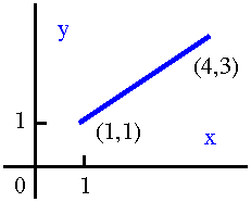 Line segment
Maybe the simplest curve is a straight line segment. Let me "find" the
length of the line segment joining (1,1) and (4,3). This should be the
same as the distance from (1,1) to (4,3), which is (square root of the
sum of the squares!) sqrt(13). Let's find this number using the
calculus formula above.
We need a formula for the line segment. The slope will be
(3–1)/(4–1) which 2/3. So f(x)=(2/3)x+something. What will the
"something" be? Since the line should pass through (1,1), when we put
x=1, the result should be 1. Therefore (2/3)(1)+something=1, so
something is 1/3. The formula is f(x)=(2/3)x+(1/3). The derivative is
f´(x)=(2/3). Now the arc length is ∫absqrt(1+[f´(x)]2)dx
which is
∫14sqrt(1+[2/3]2)dx. The
integrand is a constant, so the result is
sqrt(1+[2/3]2)x|14=sqrt(1+[2/3]2)4–sqrt(1+[2/3]2)1=sqrt(1+[2/3]2)3.
This is the same as sqrt(13).
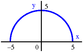 Circle
Maybe the next curve to look at is a circle, but we need the graph of
a function so let's try to find the arc length of a
semicircle. Let's look at the upper semicircle, radius 5, center at
(0,0). For this curve, f(x)=sqrt(52–x2). Now I
need sqrt(1+[f´(x)]2). So:
f´(x)=(1/2)(52–x2)–1/22x using
the Chain Rule. The 2's cancel, and we need to square the derivative,
so:
(f´(x))2=(52–x2)–1x2
but this is the same as x2
-----
52–x2 to which we must add 1:
      x2     52–x2+x2      52
1 + ----- = --------- = ------
    52–x2      52–x2     52–x2
Finally we supposed to take the square root of this result, so that
the integral we need to compute is ∫–55
5/sqrt(52–x2)dx.
This should look slightly familiar. The trig substitution x=5sin(θ) makes this integral into
∫5θ dθ=5arcsin(x/5)+C. I am skipping the
details because I've done many of these integrals already. Now
evaluate the definite integral:
5arcsin(x/5)|–55=5arcsin(1)–5arcsin(–1),
and (since I know arcsin(1)=Π/2 and arcsin(–1)=–Π/2) this works out
to 5Π, which is indeed half the circumference of a circle of radius
5.
|
Problems in the book
These two curves work out fairly well. But let's look at section 8.1,
and some of the problems there. The problems mostly have the form,
"Find the length of the graph of the function defined by the following
formula" and I think the instructions should be modified to read "the
following absurd formula." Here are some of the formulas from there:
(1/12)x3+x–1 (problem #3)
(x/4)4+(1/{2x2}) (problem #4)
x3/2 (problem #7)
(1/3)x3/2–x1/2 (problem #8)
(1/4)x2–(1/2)ln(x) (problem #9)
ln(cos(x)) (problem #10)
{ex+e–x}/2 (problem #18)
Why didn't the book ask something simpler, instead of functions
defined by such bizarre formulas? Let's see why. I will answer problem
1 of section 8.1, which asks for the arclength of y=x4
between x=2 and x=6. The problem actually asks only for the definite
integral and adds but do not evaluate.
We consider
∫absqrt(1+[f´(x)]2)dx. Here
a=2 and b=6, and since f(x)=x4,
f´(x)=4x3. The answer to problem 1 is therefore
∫26sqrt(1+16x6)dx.
What about evaluation? In the sense most often used in calculus
courses, this integral can't be evaluated. That is, there is no
antiderivative of sqrt(1+16x6) which can be written in terms
of standard functions. This isn't because we're ignorant, but because
it is impossible to do this. If you wanted to compute this
arclength, you would need to use one of the numerical techniques.
The secret to the problems in the textbook which were quoted above is
that all of the bizarre functions were selected so that
sqrt(1+[f´(x)]2) becomes something which it is
possible to integrate (in the sense of "find an antiderivative and use
FTC"). I did problem #18. Here it is.
Section 8.1, problem #18
Let's find the arc length of f(x)=(ex+e–x)/2
from x=–10 to x=10. Now
f´(x)=(ex–e–x)/2. Now let's
square.
          (ex)2  –2  +(e–x)2
(f´(x))2= ------------------
                  4
All sorts of subtle things are going on here. Notice that
(–e‐x)2
is written (e‐x)2 because the two minuses
cancel. Also notice that –2 is really
–2exe–x. Now another subtle
observation: 1=4/4. Therefore (look closely!)
               (ex)2  –2	   +(e–x)2   4 + (ex)2  –2  +(e–x)2
1+(f´(x))2= 1+ ------------------ =  ---------------------
                        4                     4
Now the top of that fraction is (ex)2 +2
+(e–x)2. Realize that 2 is
2exe–x. Notice (not an accident!)
that this top is actually a "perfect square". It is
(ex+e–x)2. So the mysterious
and almost always horrible sqrt(1+(f´(x))2) becomes,
in this case, exactly (ex+e–x)/2. Wow. The
arc length integral is
∫–1010[(ex+e–x)/2]dx
and this is (ex–e–x)/2|–1010, which is
[(e10–e–10)/2]–[(e–10–e10)/2]=e10–e–10.
These functions and these graphs
The functions quoted from the problems in section 8.1 are mostly
rather silly. This one, (ex+e–x)/2, is
not. Some pictures:
ex
Exponential growth |
e–x
Exponential decay |
(ex+e–x)/2
The average of the
two |
|---|
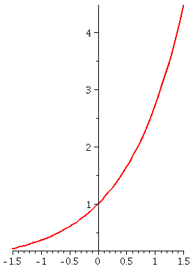 |
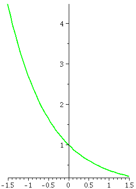 |
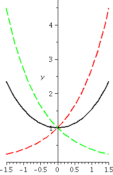 |
The curve shown in the third box is called a catenary, and it is
the curve a "uniformly loaded chain" describes. The function
(ex+e–x)/2 is called the
hyperbolic cosine and is usually abbreviated cosh(x)
(pronounced kosh ecks). Its derivative is (naturally!) the
hyperbolic sine,
(ex–e–x)/2, and is abbreviated
sinh(x) (pronounced cinch ecks). Really. We used (and proved!) the hyperbolic
function identity 1+(sinh(x))2=(cosh(x))2.
"Truth"
The truth for arc length is that, more or less, the computability of
the arc length integral using FTC and familiar functions is
impossible almost all of the time! Therefore, from the
elementary, student point of view, maybe this is all a waste of
time. But, really, it isn't. As soon as you give me a definite
integral and want to approximate the values, there are all sorts of
strategies. So what's important is that arc length can be computed by
a definite integral, and what's important for you to try to understand
is the philosophy of going from the vague idea of arc length to the
integral formula for the arc length. And that philosophy will now be
displayed again as we get an integral formula for a certain type of
surface area.
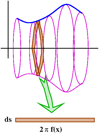 Surface area
Suppose we are again given a function y=f(x) defined on an interval
[a,b]. I would like to "compute" (the quotes are because we will get a
definite integral formula which will share the benefits and defects of
the previous result) the surface area which results when the
graph of y=f(x) is revolved around the x-axis.
We will get our formula using the same philosophical approach. We can
chop up [a,b] into many little pieces, each having length, say,
dx. Then (the picture!) the little piece of arc length laying over dx,
which we called ds, will be revolved around the x-axis. This gets us a
sort of ribbon. What is the area of that ribbon? We won't be able to
compute it exactly, but maybe we can approximate the area of the
ribbon nicely. Well, we can take the magic scissors (hey: I was able
to draw the darn scissors almost correctly this time!) and cut the
ribbon and then, sort of, almost, lay it out flat. The result will
sort of, almost, be a rectangle. What are the dimensions of this
rectangle? One side is the length of the piece of arc, ds. The other
side is the circumference of a circle whose radius is f(x), the height
of that part of the curve away from the x-axis. (The reason for the
repeated "sort of, almost" is that this is actually a distortion of
the true value - the ribbon really would not lie flat, and the ribbon
really would just approximately be a rectangle. I will try later to
address these sorts of slight (?) distortions.) So a piece of the
surface area is 2Π f(x) ds. We use a definite integral to
get the total surface area and add everything up. The result for the
area when the curve is revolved around the x-axis is
∫ab2Π f(x)sqrt(1+[f´(x)]2)dx.
Notice that sqrt(1+[f´(x)]2)dx (this uses what we had
for ds).
Sphere
Here is a result from a long time ago (thousands of years!): the
surface area of a sphere of radius R is 4Π R2. (This
is the area of four "great circles" of the sphere, circles made by
intersecting a plane with the center of the sphere.) I would like to
verify this result using the surface area formula. I'll use the same
semicircle as before: f(x)=sqrt(52–x2), with
a=–5 and b=5. Please note that revolving this semicircle around the
x-axis gets the area of the whole sphere of radius 5, so that the
answer should be 4Π(52).
We need to compute ∫ab2Π f(x)sqrt(1+[f´(x)]2)dx.
Notice that sqrt(1+[f´(x)]2)dx is what we called ds before, and we
did compute ds in a previous example. We
saw that ds was equal to 5/sqrt(52–x2)dx. But
f(x)=sqrt(52–x2) so, wow! (yeah, wow) there is
cancellation and the arclength becomes ∫–55(2Π)5dx which does indeed work out
to 100Π as it should.
More "truth"
There are very few simple powers of x (x2 and x3
and maybe x1) which give me integrands in the surface area
formula that I can find antiderivatives of. (That's a horrible
sentence!) If I want to compute surface areas for almost any "random"
function defined by a formula, I'll need to use numerical
approximations.
|
We actually ended about 4 minutes early. I owe you.
| Monday,
October 12 | (Lecture #10) |
|---|
I think lecture #10 was the exam. I will fall behind the schedule
listed in the syllabus today because I want to spend more time on
improper integrals which can be bizarre and which are important. I
also mentioned a quote from von Neumann, appropriate because improper
integrals can be so bizarre.
A quote from von Neumann
John
von Neumann (1903-1957) was a mathematician who was raised in
Hungary and spent most of his career in the United States. He worked
in many areas of pure and applied mathematics. His ideas were
influential in quantum mechanics, the development of nuclear weapons,
game theory, and the theory and construction of digital computers.
In mathematics you don't understand things. You just get used to
them.
Another kind of improper integral
The integrals we've looked at are called improper because their
domains are infinite. But there is another collection of integrals
which are also labeled improper because something goes wrong in their
ranges: the function to be integrated becomes infinite. Here are some
simple examples.
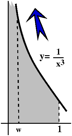
Toy example #1
Let's look at ∫01(1/x3)dx. Here
f(x)=1/x3 and surely as x→0+,
f(x)→+∞. Here is the official way to analyze this
improper integral. Suppose that w is a small positive number. Compute
∫w1(1/x3)dx. We can do this with
FTC by finding an antiderivative. The integral is
–1/(2x2)]w1=
–1/(2·12)–[–1/(2·12)]=(1/2w2)–(1/2).
Now as w→0+, certainly this→+∞. Therefore
the improper integral
∫01(1/x3)dx
diverges. Sometimes people declare that the integral "diverges to
infinity".
The picture accompanying this is, again, useless. It helps me to
organize the computation, but does not show enough quantitative
information to help decide convergence or divergence.
Toy example #2
Let's look at ∫01(1/sqrt(x))dx.
This does converge and its value is 2. Why?
Suppose that w is a small positive number. Compute
∫w1(1/sqrt(x))dx. We can do this with
FTC by finding an antiderivative. The integral is
2sqrt(x)]w1=
2sqrt(1)–2sqrt(w).
Now as w→0+, certainly this→2.
Therefore we say that the improper integral ∫01(sqrt(x))dx
converges and its value is 2.
I tried to change things a bit after we considered these examples. So
what about ∫01((1+ex)/x3)dx? Does this
converge or diverge? We can compare this to Toy Example
#1. Indeed, I know that for all x in the unit interval (actually,
inside the unit interval, since x≠0) 1+ex>1, so that
(1+ex)/x3>1/x3. So the
"area" under y=(1+ex)/x3 is larger than the area
under y=1/x3. But the latter area, by the analysis in Toy
Example #1, is infinite, so the larger area must also be infinite. So
this is good: without much work, we can conclude that the improper
integral ∫01((1+ex)/x3)dx diverges. Of
course you can complain to me that I arranged this example. I will
certainly agree with that, but we need to walk before we can run. And
we need to run before we fall down and get hurt a lot. (No, I don't
think that last sentence is part of efficient, warm educationese.)
How about ∫01(1/[sqrt(x)+x3])dx? Here we know that
0≤>(1/[sqrt(x)+x3])≤1/sqrt(x). But
∫01(sqrt(x))dx does converge -- it has
finite area. So a smaller set, the one designated by
∫01(1/[sqrt(x)+x3])dx, will also converge.
Both of these computations are examples of a comparison technique,
a nice indirect way to conclude that certain improper integrals
converge. Here is one statement of this comparison technique.
Comparison for Improper Integrals
Suppose I know that 0≤f(x)≤g(x) for all x with 0<x≤A.
If ∫0Ag(x)dx converges, then
∫0Af(x)dx converges. The value of
this integral will be at most the value of the first integral.
If ∫0Af(x)dx diverges, then
∫0Ag(x)dx diverges.
(Convergence is "inherited" downwards, and divergence is inherited
upwards. In general, the other implications (the converses) are not
true.
A Maple dialog
Here is a record of a Maple session I
just created.
> int(1/x^3,x=0..1);
                                   infinity
> int(1/sqrt(x),x=0..1);

                                       2
> int((1+exp(x))/x^3,x=0..1);
                                   infinity

> int(1/(sqrt(x)+exp(x)),x=0..1);
                                1
                               /
                              |         1
                              |   ------------- dx
                              |    1/2
                             /    x    + exp(x)
                               0
> int(1/(sqrt(x)+exp(x)),x);
                               /
                              |        1
                              |  ------------- dx
                              |   1/2
                             /   x    + exp(x)
> int(1/sqrt(x),x=0..(.001));
                                 0.06324555320
> int(1/(sqrt(x)+exp(x)),x=(.001)..1);
                                 0.4636551521
Discussion of what was typed
The first two entries and responses show that
Maple
knows a bit about improper integrals.
The next lack of sensible response shows that the program can't
contribute to the integration of 1/(sqrt(x)+ex) on [0,1]
and the response following exhibits
Maple's lack of ability to find an
antiderivative of the integrand. But we can compute (if by
compute we mean approximate)
∫011/(sqrt(x)+ex)dx. We
write
∫011/(sqrt(x)+ex)dx=∫0s1/(sqrt(x)+ex)dx+∫s11/(sqrt(x)+ex)dx
Now we estimate
∫0s1/(sqrt(x)+ex)dx since
1/(sqrt(x)+ex)<1/sqrt(x). Well,
∫0s1/(sqrt(x))dx=limw→0+∫ws1/(sqrt(x))dx=limw→0+2sqrt(x)]ws=limw→0+2sqrt(s)–2sqrt(w)=2sqrt(s).
So if we really want to compute, we could just select s so that the
"singularity" is cut off by choosing s so small that 2sqrt(s) is less
than half of some error. Then we could use a numerical routine to
compute the "other piece",
∫s11/(sqrt(x)+ex)dx, since this
is a proper (!) integral, again to half the error tolerance. The
reason for half of the error in each piece is that we add up the
pieces and the errors might reinforce.
The last two Maple instructions tell me
that ∫011/(sqrt(x)+ex)dx is 0.46
with .06 as an overestimate of the error. You may think this is
bizarre, but this strategy works and it is fairly simple.
Here is one part of the session I didn't discuss in class. I did this
immediately before class, and I was a bit startled by the result. Look
at it, please.
> int(1/(x^3+sqrt(x)),x=0..1);
     /              1/2
     |             5    - 1       1/2          1/2 1/2                     1/2 1/2          1/2 1/2
1/20 |8 arctan(----------------) 5    (10 - 2 5   )    + 10 ln(2) (10 + 2 5   )    (10 - 2 5   )
     |                  1/2 1/2
     \         (10 + 2 5   )

                     1/2                                                     1/2
                    5    + 1       1/2          1/2 1/2                 5 + 5          1/2          1/2 1/2
     + 8 arctan(----------------) 5    (10 + 2 5   )    - 12 arctan(----------------) 5    (10 + 2 5   )
                         1/2 1/2                                             1/2 1/2
                (10 - 2 5   )                                       (10 - 2 5   )

                     1/2
                    5    - 3       1/2          1/2 1/2       1/2       1/2          1/2 1/2          1/2 1/2
     + 4 arctan(----------------) 5    (10 + 2 5   )    + ln(5    + 3) 5    (10 - 2 5   )    (10 + 2 5   )
                         1/2 1/2
                (10 - 2 5   )

                          1/2                                             1/2
                    -5 + 5          1/2          1/2 1/2                 5    + 3               1/2 1/2
     - 12 arctan(----------------) 5    (10 - 2 5   )    + 20 arctan(----------------) (10 - 2 5   )
                          1/2 1/2                                             1/2 1/2
                 (10 + 2 5   )                                       (10 + 2 5   )

                          1/2                                            1/2
                     5 + 5                  1/2 1/2                -5 + 5                  1/2 1/2
     + 20 arctan(----------------) (10 + 2 5   )    - 20 arctan(----------------) (10 - 2 5   )
                          1/2 1/2                                        1/2 1/2
                 (10 - 2 5   )                                  (10 + 2 5   )

          1/2          1/2 1/2          1/2 1/2         1/2              1/2   1/2          1/2 1/2          1/2 1/2
     - 2 5    (10 - 2 5   )    (10 + 2 5   )    ln(5 - 5   ) + 2 ln(5 + 5   ) 5    (10 - 2 5   )    (10 + 2 5   )

                      1/2
                     5    - 3               1/2 1/2    1/2          1/2 1/2          1/2 1/2      1/2
     - 20 arctan(----------------) (10 + 2 5   )    - 5    (10 - 2 5   )    (10 + 2 5   )    ln(-5    + 3)
                          1/2 1/2
                 (10 - 2 5   )

                     1/2
                    5    + 3       1/2          1/2 1/2        1/2               1/2 1/2          1/2 1/2
     + 4 arctan(----------------) 5    (10 - 2 5   )    - ln(-5    + 3) (10 - 2 5   )    (10 + 2 5   )
                         1/2 1/2
                (10 + 2 5   )

                                                     \
           1/2               1/2 1/2          1/2 1/2|   /           1/2 1/2          1/2 1/2
     - ln(5    + 3) (10 - 2 5   )    (10 + 2 5   )   |  /  ((10 - 2 5   )    (10 + 2 5   )   )
                                                     | /
                                                     /
This took quite a lot of time (about 1.5 seconds) and memory (almost
70 megabytes). I think that Maple
computed this with a rationalizing substitution. I was surprised that
an explicit answer was given. The numerical value of this (extensive?)
answer is (approximately!) 1.776627144. I know the original integral
converges by comparing it with the 1/sqrt(x) integral, and also I know
that the value of the integral will be less than 2. And 1.77662... is
certainly less than 2.
|
L'H
I wrote a version of L'Hôpital's Rule on the board, since I would need
it twice in the next few minutes. I copied it from the book (page 272).
L'H Suppose f(x) and g(x) are differentiable functions inside
an interval containing a and that f(a)=g(a)=0. Also assume g (x)
is not 0 for x near but not equal to a. Then f(x) f´(x)
lim ------ = lim ------
x→a g(x) x→a g´(x)
if the limit on the right-hand side exists. This result is also valid
if both of the limits of f(x) and g(x) as x→a are +∞ or
–∞.
It is very important that there is a quotient in the algebraic
form. Also, the symbolic quotients 0/0 or ∞/∞ are
sometimes called indeterminate forms.
I applied this to two examples:
limx→2(x2–3x+2)/(x2–4) and
something like
limx→1(ex–x)/x2.
limx→2(x2–3x+2)/(x2–4)
Please notice that both the top and the bottom are 0 when x=2,
since 22–3·2+2=4–6+2=0 and
22–4=0. Therefore we can use L'H, which is the beginning
calculus student's dream of the product rule. The resulting quotient
is (2x–3)/(2x) and the limit of that as x→2 is
(4–3)/(2·2)=1/4.
There is another, more elementary way, to do this, since the top and
bottom are simple and can be factored:
(x2–3x+2)/(x2–4)=[(x–2)(x–1)]/[(x–2)(x+2)]=(x–1)/(x+2)
and certainly the limit of the last quotient can be obtained by
"plugging in" (more politely, "instantiating x at 2") since the
functions involved are continuous. The resulting limiting value is again
1/4.
limx→1(ex–x)/x2
Here we take the derivative of the top and bottom and a quotient is
gotten: (ex–1)/(2x), and we could indeed take more
derivatives and get (ex/2. Then plugging in to all three
quotients gets (e–1)/12=e–1 and (e–1)/2 and e/2. Of course,
the use of L'H is wrong. The original quotient does not satisfy
the eligibility criterion for L'H. There is no "indeterminaste
form". This error is easy to make since L'H is such a tempting
technique. Please: always check for eligibility first.
Sometimes some algebraic manipulation is needed to apply L'H (this
will be true in what follows). And sometimes L'H needs to be used more
than once (if the original indeterminate form is, after the
differentiation step, again an indeterminate form, etc.).
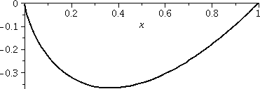 x·ln(x)
I asked people for the graph of y=x·ln(x) on the interval
[0,1]. Some people were willing to use their graphing calculators. A
graph much like what is shown to the left was produced.
The graph seems to be a slightly assymetrical bump below the x-axis,
hanging from (0,0) and (1,0). The "bottom" is at, about, –1/3
(near x=1/3, actually). We actually found the exact "bottom" by
looking at the derivative of x·ln(x): it was at (1/e,–1/e). If
you "ask" your computer or calculator for the value of x·ln(x)
at x=0, however, there will be some sort of complaint rather than a
number. The machines have been advised that 0 is not in the domain of
ln. But the graph certainly seems to indicate that (0,0) is there
(wherever there is!). What's going on?
L'H
Really what the graph indicates is a suggested value for
limx→0+x·ln(x). The guess for this is
0. To verify this guess (in a math course!) we will use
L'Hôpital's Rule. As x→0+, we have a 0 multiplied by (–)
∞. L'Hôpital's Rule works on quotients, so we need to rearrange things algebraically. Here we go:
limx→0+x·ln(x)=rearranging=limx→0+[ln(x)/{1/x}]=using L'H=limx→0+[{1/x}/{–1/x2}]=rearranging back=limx→0+–x=0
so the limit is verified.
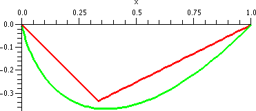 The integral
How much "area" is included in the bump above? More precisely, what is
the definite integral of x·ln(x) from 0 to 1. The bump is below
the x-axis so this integral should be negative. It sort of resembles a
triangle with base [0,1] and altitude about 1/3. So a guess is
that the area should be about –1/6. An actual
graph of the function and of this approximating
triangle is shown to the right. The function is concave down so
it bulges beneath the triangle. And, in fact, the "point" of the
triangle is above the graph. So there is more (absolute value!) area
in the bump than in the triangle.
Let's compute. The area is
∫01x·ln(x)dx. This is officially an
improper integral (it really is difficult to evaluate the integrand at
x=0!). So first I'll compute
∫Q1x·ln(x)dx for Q small positive,
and then let Q→0+. To use FTC we need an
antiderivative of x·ln(x). Integration by Parts again works. If
u=ln(x), then dv=x dx, and du=(1/x)dx and
v=(1/2)x2. So:
∫x·ln(x)dx=(1/2)x2ln(x)–∫(1/2)x2(1/x)dx=(1/2)x2ln(x)–(1/4)x2+C
The definite integral is
(1/2)x2ln(x)–(1/4)x2|Q1=((1/2)Q2ln(Q)–(1/4)Q2)–((1/2)12ln(1)–(1/4)12).
L'H
I know that limQ→0+–(1/4)Q2=0 because
Q2 is continuous and I can just "plug in". What about
limQ→0+(1/2)Q2ln(Q)? Here we (officially!) need
L'Hôpital's Rule again. So:
limQ→0+(1/2)Q2ln(Q)=rearranging=limQ→0+(1/2)[ln(Q)/{1/Q2}=using L'H=limQ→0+(1/2)[1/Q}/{–2/Q3}=rearranging back=limQ→0+(–1/4)Q2=0.
If you now put everything together (and don't lose track of the minus
signs!) you can see:
∫01x·ln(x)dx converges and its
value is –1/4. The –1/4 is certainly consistent with the estimate we
made earlier, backed up by the red and green graph.
A real application ...
This strange function with its somewhat strange graph is related to a
function used in applications. The function used in applications is
actually a bit more complicated (sigh). Here is how to think about it.
|
A graph of y=x·ln(x) on [0,1]. The function is concave up and below the x-axis. The area is –1/4, as just computed.
|
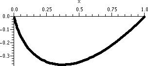
|
|
Flip the curve over the x-axis. So this is
a graph of y=–x·ln(x) on [0,1]. The function is concave down and above the x-axis. The area is +1/4, because now the region we're considering is above the x-axis.
|
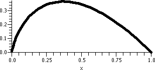
|
|
This is a more complicated flip. Replace x by 1–x. This is a flip which exchanges left and right because of the +/– change in the x multiplier. In fact, the left and right are exchanged, and the y-axis and x=1 are interchanged.
So this is a graph of y=–(1–x)·ln(1–x) on [0,1]. The function is concave up and above the x-axis. The area is 1/4.
|
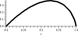
|
|
Now add up the two previous functions. Here is a graph of
y=–x·ln(x)–(1–x)·ln(1–x) on [0,1]. Yes, it
is weird. This function officially has two strange behaviors,
at both 0 and 1. The function is called the binary
symmetric entropy function and it is used to study the amount of
information flowing through a "channel" (you could think of a channel
as a wire, and the information as 0's and 1's -- bits). The entropy
function helps to analyze what happens in complicated situations where
there may be interference (noise). This function has one bump, and its total
area is 1/2.
|
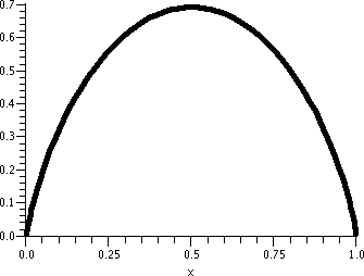
|
Comment
You can't actually predict that the result of adding the two bumps
would be just one symmetric bump. In fact, that result may not occur.
|
Here is a graph of x[ln(x)]2 on [0,1]. Because of the
square, the function is positive, and the bump is more pronounced.
| And this is a graph of x[ln(x)]2+
(1–x)[ln(1–x)]2. So two distinct bumps
can show up. |
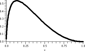 |
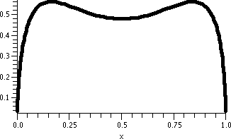 |
|
Return of the exam
Here is the first exam in a
somewhat more compact form, with one version of the answers also available. A discussion of the grading
of the exam and the results is here. Let me
make some comments about how this exam did and did not resemble a
standard 152 exam.
- Problem 1 Standard, except for the use of the parameter,
C. The problem with C resembles slightly one of the homework or
workshop problems (the one with C–x2). This is, without C, a nice
152 exam problem.
- Problem 2 Standard problem.
- Problem 3 This is an easy computation but a difficult idea
to explain. (The computation is so easy that several people
essentially seemed to refuse to do it!) This is a possible 152
problem, but slightly more conceptual than usual (although I did give
a rapidly vibrating (sin(Nx))3 as n→∞ as a 152 exam problem).
- Problem 4 A difficult problem -- some people not in the
class were interested that I asked this question. Almost half the
students got it entirely correct and many others got most credit. I
was impressed.
- Problem 5, 6, and 7 Routine 152 exam problems.
- Problem 8 Mostly routine, but, of course, the estimate is
somewhat irritating. I would give this problem in a standard 152
course, but not expect great performance.
| Monday,
October 5 | (Lecture #9) |
|---|
Goethe
Here is
Maxim #1005 from
Maximen und Reflektionen written by Johann Wolfgang von Goethe,
German dramatist, novelist, poet, & scientist (1749-1832) with a
precise quote and a precise translation:
Die Mathematiker sind eine Art Franzosen: Redet man zu
ihnen, so �bersetzen sie es in ihre Sprache, und dann ist es alsobald
ganz etwas anders.
As translated by a native speaker:
Mathematicians are some sort of Frenchmen: if you talk to them, they
translate it into their language, and then it is soon something
completely different.
This was to alert you that when you meet and "use" mathematicians, you
should realize that they will try to find out what the rules of the
(logical) game are and then, maybe, change and break them. Sometimes
this is just for fun (!) and can be sort of useless. But sometimes
breaking the rules can be in response to needs for additional
mathematical tools. We consider that kind of rule-breaking today.
Improper integrals: what are they?
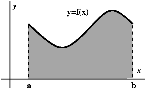 So far we have
discussed computing standard definite integrals. Although certainly a
definite integral like ∫abf(x)dx can represent many different
ideas, the most familiar instantiation is as an area (assuming that
f(x)>0 for x in [a,b]) bounded by the x-axis, x=a, x=b, and the
graph of y=f(x). In most of the computations we've done, the function
f has been rather "nice" -- differentiable, mostly, and only a few
times has it had some discontinuities. In fact, there are many
applications where this simplicity is made more complicated because
the applications themselves demand a
"stronger" kind of integral.
|
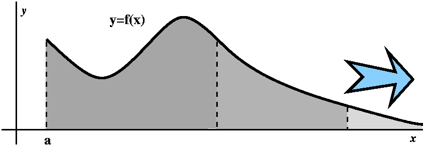 For example, we might consider a situation where, say, b gets larger
and larger and
larger. Where, say, b→∞. I will give a real physical example of this at the next
lecture. This integral will have a domain which is an infinite
interval. It could be [a,∞) or
(–∞,b] or even (–∞,∞). Such integrals also occur very frequently in statistics
(and therefore they "infiltrate" almost all experimental sciences!).
A completely naive interpretation of the area would declare
that since the length of the base is infinite, the total area must
somehow be forced to be infinite. More subtly, the height in certain
cases will decrease fast enough so that the total integral can be
thought of as finite.
|
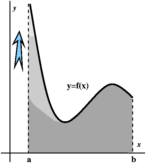 There may also be a sort of defect (?) in the range of f. For
simplicity, consider the situation where, although f is "nice" for
x>a, as x→a+, f(x) gets larger and
larger and larger: in fact, we might need
to try to "integrate" or compute the value of ∫abf(x)dx even if
f tends to ∞ as x→a.
Again, a first look could convince you that such "areas" need to be
infinite, also, because the height is infinite. But, actually, the way
f grows as x→a+ is what matters. It is possible to
imagine that the growth of f is so controlled that the total
approximating areas don't tend to ∞. And maybe, in such
situations, we should be able to compute the integral.
I will first consider the "defect in the domain" case.
Toy example #1
Look at y=1/x2. The integral ∫1B(1/x2)dx (I'm using B as an
abbreviation for BIG) can be computed directly:
∫1B(1/x2)dx=–1/x|1B=1–(1/B) (be careful of the signs!)
Now if B→∞, certainly
1–(1/B)→1. Then we will declare that the improper integral
∫1∞(1/x2)dx converges and its value is 1.
Toy example #2
Look at y=1/x. Consider the analogous integral ∫1B(1/x)dx (again think of B as
a BIG number). We compute it:
∫1B(1/x)dx=ln(x)|1B=ln(B)–ln(1)=ln(B)–0
I wanted also to consider here the behavior as B→∞, but some students seemed to be
confused (this is confusing!). What does happen to ln(B) when B
gets large? If you only have a loose idea of the graph in your head,
well the log curve might not look like it is increasing too
fast. Well, it actually is not increasing very fast, but it is
increasing. Look: ln(10) is about 2.3, so ln(102)=2ln(10)
is about 4.6 (that's 2·2.3), and ln(103)=3ln(10) is
about 6.9 (that's 3·2.3), etc. Here etc. means I can get values
of ln as large as I want by taking ln's of large enough powers of 10
(hey, ln of 105,000 is bigger than ... 10,000: so
there!). So the values of ∫1B(1/x)dx do not approach a specific number as B→∞. Therefore we say:
the improper integral
∫1∞(1/x)dx diverges.
The distinction between converges (approaches a specific finite limit)
and diverges (does not approach a specific finite limit) is the one
that is important in applications and that motivates the distinct use
of the two words.
Geometric constrast
I love pictures. I like computation, but I can barely tolerate (!)
"algebra". But I introduced the actual definition of {con|di}vergent
improper integrals with some algebra, and didn't draw any
pictures. Why? Well, because pictures, while useful, don't help too
much. Here are qualitative pictures of the
two graphs.

Well, they are actually different graphs, sorta. But I wanted
to emphasize, through sketching them not too carefully (and on
different axes, without scales!) these curves both "start at" (1,1),
and as they go right, are always positive, decreasing, concave up,
with 0 as limits. My eyes, at least, can't tell that one of them (on
the left?) has finite total area, and one of them (to the right!) has
infinite total area. The difference is quite surprising.
The exponential probability distribution
 Many real-life phenomena are described using something called the
exponential probability distribution. For example, the probable life-time of a lightbulb could be described with it. See here for more information.
I will just discuss lightbulbs now. Here is a first attempt to
be precise. If the probability that a light bulb will fail in t
minutes is proportional to e–Ct then the lifespan of the
bulb is said to have an exponential probability distribution. More
specifically, if t=0 is NOW, and t1<t2 are
later times, then then the probability of lightbulb failure between
the times t1 and t2 is proportional to ∫t1t2e–Ctdt.

That is, that portion of the area to the right which is shaded
blue represents the chance of a lightbulb burning out during that
particular time interval.
What is the total probability from NOW to FOREVER?
Every (real!) lightbulb is going to fail some time. Probabilities of
an event range from 0 to 1, where an event which is certain
will have probability 1. Since any lightbulb will fail between t=0
(NOW) and t=∞ (FOREVER), we should consider the (improper)
integral ∫0∞e–Ctdt. Let me analyze this carefully.
Suppose A is a large positive number. Let's compute ∫0Ae–Ctdt=–(1/C)(e–Ct)]0A=–(1/C)e–CA+(1/C)e0=(1/C)–(1/C)e–CA.
The antiderivative has a –(1/C) factor because when e–Ct is
differentiated, the Chain Rule produces a multiplicative –C, and the
–(1/C) cancels this. Now what happens to (1/C)–(1/C)e–CA as
A gets large, A→∞? e–CA (with a negative sign,
with A and C positive) must go to 0 (this is exponential
decay). Therefore the improper integral ∫0∞e–Ctdt converges,
and its value is 1/C. But, wait: since every lightbulb fails,
shouldn't this be 1? Yes, surely. Let's fix this up. The key is
"proportional to". We should multiply the function e–Ct by
a constant so that the improper integral will turn out to be 1. The
computation we just did shows that the constant should be C. So the
probability distribution is actually Ce–Ct.
The {expectation|mean|average} of an exponential probability
distribution
Let me try to discuss something a little bit harder. First, some
background with (maybe) some easier ideas. We could imagine a
population of, say, bugs. Maybe there are three types of bugs in
my bug collection and I know the following information:
| My bug collection |
|---|
| Bug type | Observed lifespan | Proportion in
my collection |
|---|
| Orange spotted bug |
20 days |
30% |
| Blue striped bug |
50 days |
50% |
| Red plaid bug |
80 days |
20% |
What is the average lifespan of this bunch of bugs? Well, it isn't the
average of the 3 lifespans (the sum of 20, 50, and 80 divided by 3 --
a rather naive computation) since that doesn't take into account the
varying proportions of the bug types. If you think about it, the
average in this case is
20·(.3)+50·(.5)+80·(.25): a sort of weighted sum. It is a
sum of lifetimes multiplied by the proportion of the population. You
should convince yourself that this is the correct number.

What about lightbulbs? What proportion of a lightbulb population will
"die" at time t? Well, that proportion is about
Ce–Ctdt. The appropriate weighted sum in this case
multiplies the proportion by t and adds it all up with an integral:
∫0∞tCe–Ctdt. If we
compute this integral, we maybe can get some idea of when an average
lightbulb dies. This quantity is called the mean or the expectation.
We can compute ∫tCe–Ctdt using integration by parts. If u=t then
dv=Ce–Ctdt and du=dt and v=–e–Ct. Therefore
uv–∫v du is
–te–Ct–∫–e–Ctdt=–te–Ct–(1/C)e–Ct.
The definite integral from t=0 to t=A is
–te–Ct–(1/C)e–Ct]0A=–Ae–CA–(1/C)e–CA–{–(1/C)e0}.
What happens at A→∞? Well, e–CA certainly goes to
0 (radioactive decay!). But the term Ae–CA has a sort of
conflict. Although the exponential decays, certainly A→∞?
Which factor "wins"? Exponential decay is faster than any degree of
polynomial growth, actually, so the limit is 0. You certainly can see
this with L'Hopital's rule:
limt→∞te–Ct=limt→∞t/[eCt]=limt→∞1/[Cexp(Ct)]=0.
So the integral from 0 to A, as A→∞, approaches a limit,
which is –{–(1/C)e0}=(1/C). This is the average
lifespan of a lightbulb. Incidentally, if we want to check that this
is a valid model, we can look at sample lifespans, and this can be
used to identify the value of the parameter C. The average lifespan
written on a package I just examined is 750 hours. Other technical
words which refer to average lifespan are mean and
expectation.
Other things ...
People who study statistics are interested in more details about life
and lightbulbs than are described here. For example, they may want to
know how dispersed the lifespans are around the mean. That is,
do all of the lightbulbs tend to die out right around 1/C, or is there
a considerable amount of variability? Various numbers measure this,
including variance and standard deviation. They all need computation
of ∫0∞t2Ce–Ctdt, a
different improper integral.
|
Here is an extended example of how to use improper integrals in a
physical setting. I've used this example in our 152 instantiations,
but don't have time this semester.
Escape velocity
When I was very young, I read a science fiction novel by Robert
Heinlein which stated "... the escape velocity from the Earth is 7
miles per second ..." and now I would like to sort of verify this
using only well-known (?) facts and some big ideas of physics.
|
The radius of the earth
Well, a sketch of the (continental)
United States is shown to the right. There are 4 time zones. The
U.S. is about 3000+ (maybe 3200?) miles wide. Therefore one time zone
is about 1000 miles wide (I think the Pacific time zone actually slops
a bit into the ocean), and since there are 24 time zones around the
world, the circumference of the world is ... uhh ... about 25,000
miles. Or so. And therefore the radius of the earth is that divided by
2Pi, and therefore the radius of the earth is about 4,000 miles.
|  |
Newton and gravitation Two masses attract each other with a force
whose magnitude is proportional to the product of the masses and
inversely proportional to the square of the distance between
them. Therefore, if I have a mass, m, and if the Earth has mass M, the
magnitude of the force of gravity is GmM/r2. G is a
constant.
Work lifting up Suppose we want to lift a mass m from the surface
of the earth to a distance R, where R is very large. Then the work
done is force multiplied by distance. The force needed to act against
gravity certainly changes with distance. So I will compute the work
with calculus. If x is some distance between 4,000 and R, then the
force is GmM/x2. If the distance is a little bit, say, dx,
then the work dW needed is GmM/x2 dx. The total work,
W, is ∫x=4,000RGmM/x2 dx which
I can compute readily as –GmM/x]4,000R=GmM({1/4,000}–1/R). I
think I did the minus signs correctly. Notice that as R→∞,
this work →GmM/4,000: this is the most work you can do, to get
anywhere in the universe (assuming the universe is empty except for
the mass m and the earth, of course).
Kinetic energy How much kinetic energy would we need to supply
to the mass m so that it would equal the potential energy the mass
would have if it were lifted out to anywhere in the universe?
Well, kinetic energy is (1/2)mv2 and that potential energy
we already computed is GmM/4,000. So (1/2)mv2=GmM/4,000,
and thus v2=2GM/4,000. But what is GM?
But F=ma On the earth, a, the acceleration of gravity, is 32
ft/(sec)2. Yes, this is an archaic system of measurement,
but that's part of the fun. But also F=GmM/(4,000)2. So
GmM/(4,000)2=32m. Therefore
GM=(4,000)2·32.
And the answer is
...
v2=2GM/4,000=2[(4,000)2·32]/4,000=8,000·32=
(256,000)/(5,280)=(approximately)50. The 5,280 came from converting
feet to miles. Therefore v, the escape velocity, is about 7mps. I think
this computation is so silly that it is cool.
|
Maintained by
greenfie@math.rutgers.edu and last modified 10/13/2009.
 An infinite series ∑n=1∞an can
be thought of as ∑n=1Nan+∑n=N+1∞an. So
there is the Nth partial sum plus the "other" terms of the
series, an infinite tail. These other terms I may sometimes call
TN. I like to think of this maybe as some sort of
animal. The partial sum is the body, and the infinite tail is
... well, the tail. The question of whether the series converges or
not maybe is analogous to whether the whole weight of the animal is
finite (this is a good analogy only for series whose terms are all
positive -- we will deal later with series whose terms change
sign). The weight will be finite exactly when the infinite
tails→0 as n→∞. In fact, the first "few" terms of a
series have
nothing to do with convergence! You can change them, and the
convergence of the series won't change at all. (If the series
converges, the sum will change, but whether or not the series
converges won't be changed.)
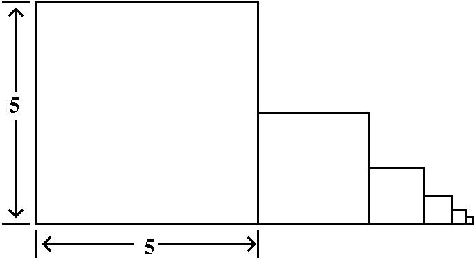 Example #2
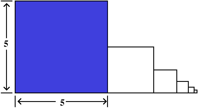
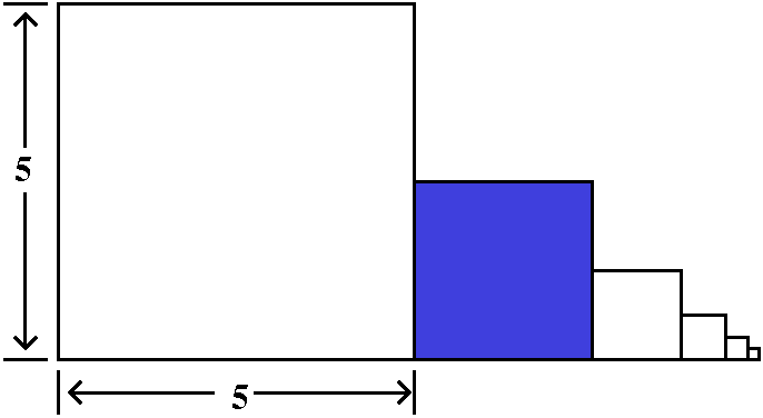
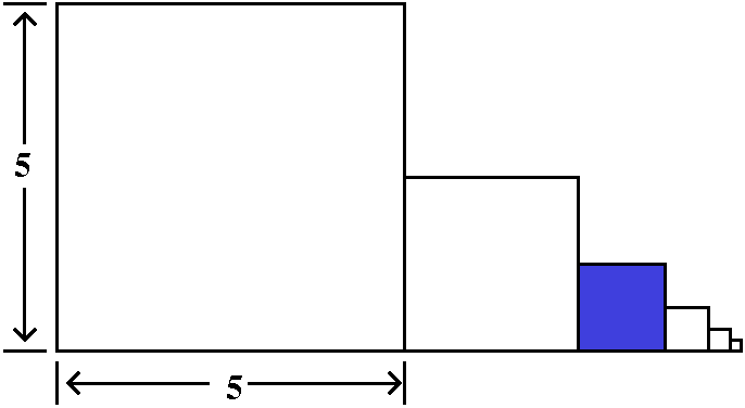
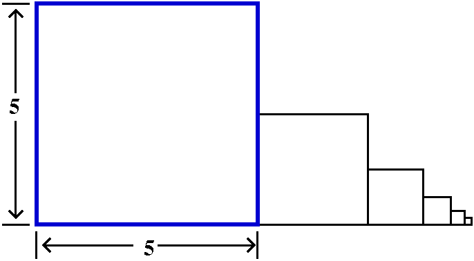
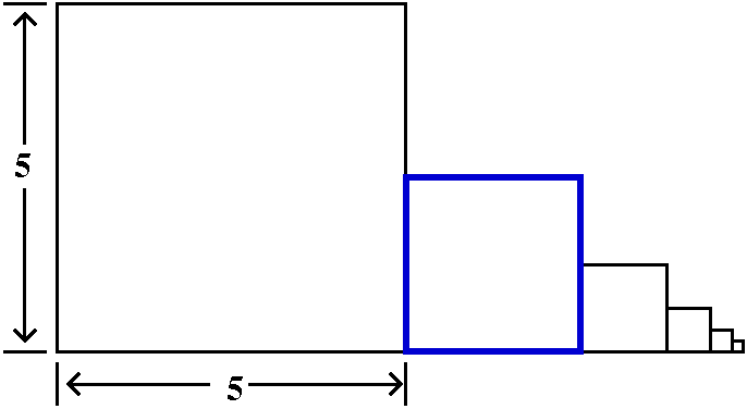
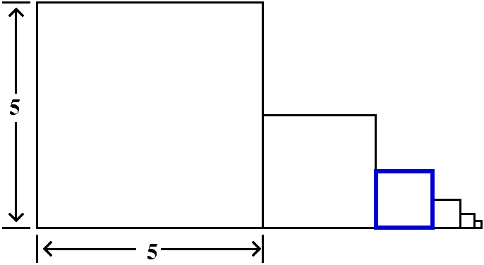
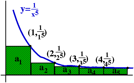 Comparison to a definite integral
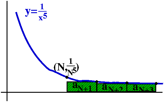 Here is how to overestimate this TN. Look at the picture to
the right. The curve y=1/x5 is again there, and I am
interested in what happens for x's bigger than N. I put the boxes
representing TN (remember, this starts with
1/(N+1)5) under this portion of the curve. So (very very
tricky!) I can make this estimate:
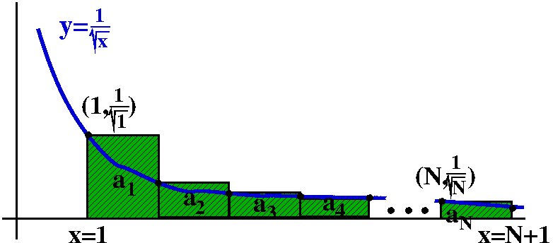 A partial sum bigger than 100
 What happens?
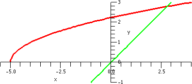
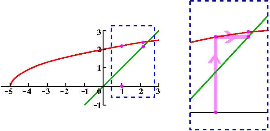
 Maybe sometimes we might think of a picture of the sequence, but this
really has limited use as you will see. To the right is a picture of
the first 6 elements of the sequence {1/n}, sitting on the number line.
 A rudimentary picture of the sequence is shown
to the right. Notice that there is something missing from this
sequence -- the dynamic aspect as the sequence wiggles and hops left
and right. Every element of the sequence is in the picture and the picture isn't very helpful to me at all. Does this sequence converge? Historically an answer to this
question wasn't obvious. People finally decided that the answer should
be no. The only numbers that are authentic candidates for the limit of
this sequence are 1 and –1. If we were going to use sequences as ways
of getting better and better approximations to a root of an equation,
then saying that the root is maybe 1 or maybe –1 is probably not the
best answer. People usually want one specific answer. So the
definition of limit, even if we want only to consider it informally,
needs to be stated slightly differently.
 Let's look at the sequence {51/n}. The first few terms, in
decimal form, are these: 5., 2.236067977, 1.709975947, 1.495348781,
1.379729661, 1.307660486, 1.258498951. A picture of the first 6 of
these is to the right. Maybe things here are not totally clear. In
fact, one of the reasons I want to discuss this example is that things
are not clear. We made some preliminary observations: certainly
any root of 5 would have to be positive, in fact any root would have
to be bigger than 1. And also any root would have to be less than
5. So what we know is that 1<51/n<5. The numbers in
the sequence are "trapped" inside the interval from 1 to 5. I asked
the class if just knowing this information was enough to guarantee
that the sequence converged. After some thought, one student came up
with the following example: {3+(–1)n}. Again depending on
parity, the values of this sequence are either 2 (n odd) or 4 (n
even). This sequence does not converge although its values are inside
the interval from 1 to 5.
 I looked at this error estimate for f(x)=x1/3, n=3, a=8,
and x in the interval [6,8]. I chose an interval centered at 8 so that
|x–8|≤2. To the right is a picture containing graphs of both y=x1/3 and y=T3(x) as x goes from 0 to 16.
 To the right is another picture. Look at it very carefully
please. It is also a graph of both y=x1/3 and y=T3(x) as x goes from 6 to
10. Both curves are displayed. But I can only see one
curve. Maybe if I look really really really closely, maybe I can see
some dots of two colors but I am not sure. How close are these curves?
 Therefore the error is at most (.0014)(16/24) and this is about
.00092. Now look carefully at the picture. Do you think you can
see a difference in height of less than .001? The difference
between two of the "hashmarks" on the vertical scale is .05, and the
graphs of the functions are separated by one-fiftieth (that's 1/50) of that
difference. I don't think that the pixels in the picture are small
enough to show this!


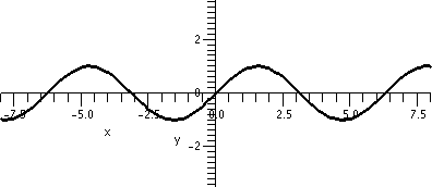 How can we compute values of the sine function? Here's a graph, but
even producing this graph requires a computer to get many values of
sine and then use them to pick out and color certain pixels. We could
construct a bunch of triangles, measure angles and lengths
carefully, and then get some values of sine. This is, more or less,
how things were done in Egypt and Greece. Certainly it is an intricate
process and very difficult to implement. But hundreds of years later,
a more systematic and accurate method was developed, first in India,
and then in Western Europe. The history in India was long
ignored. Here's
 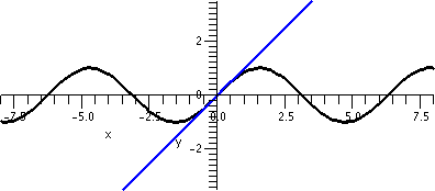 The start of this game is to look again at the tangent line
approximation which was discussed in calc 1. Let's try to
approximate sin(x) locally near 0. The tangent line goes through (0,0)
since sin(0)=0 (hey: one value of sine which is easy to know!) and it
has slope 1 since the derivative of sine is cosine and cos(0)=1. For
x's near 0, look at the picture, and realize that sin(x) will be
approximately equal to x.
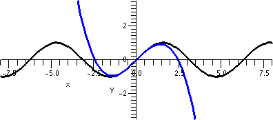 Now I displayed a mysterious (?) cubic (third degree) polynomial. It
turns out that this polynomial comes from a rather simple process, one
that can be described easily and efficiently to a computer or
calculator. In fact, it is a process which is simple enough so that
computations can be done by hand, as they were for several
centuries. The picture shows that the cubic polynomial stays closer to
sin(x) in a larger interval than the linear approximation, x, does. I
can't show you also a sort of microscopic picture, but I do assert
that cubic polynomial is a better approximation to sin(x) than just x alone. I'll give some numbers.
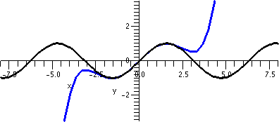
 So I'm skipping a few polynomials and jumping up to the 9th
degree approximation. The numbers may look a bit strange (you will
get used to them!).
 Modeling this story to solve the problem
 The implicit form of the equation is therefore
ln(T–30)=(1/10)ln(1/5)t+ln(250). Let's exponentiate, and use
exponentiation properties and log properties:
 An explicit form of the solution is
y=[2e2x]/[1+e2x]. This may be in a form that
"real people" can understand.


 Stable equilibrium
 Unstable equilibrium


 An example: y´=y2


 The idea of polar coordinates

 If you consider the picture to the right, I hope that you can fairly
easily "read off" how to go from r and θ to x and y:


 The rectangular graph of 1+sine, shown here, decreases
down to 0 and then increases to +1. The polar graph dips to 0 and then
goes back up to 1. The dip to 0 in polar form is geometrically a sharp
point! I used "!" here because I don't believe this behavior is easily
anticipated. The technical name for the behavior when r=3Π/2 is
cusp.

 The rectangular graph on the interval [0,2Π] of sine moved up by 1/2
shows that this function is 0 at two values, and is negative between
two values. The values are where 1/2+sin(θ)=0 or sin(θ)=–1/2. The values of θ satisfying that equation in the
interval of interest are Π+Π/6 and 2Π–Π/6. The curves goes down to
0 distance from the origin at Π+Π/6, and then r is negative until
2Π–Π/6. The natural continuation of the curve does allow negative
r's, and the curve moves "behind" the pole, making a little loop
inside the big loop. Finally, at 2Π–Π/6, the values of r become
positive, and the curve links up to the start of the big loop.


 The rectangular graph, shown here, has three pairs of ups
and downs. The polar trace covers the leaves twice. The six
up-and-downs of cos(3θ) (magically?) reduce to retracings of
half of the loops. I hope I made this evident. I
introduced some deliberate distortion in the second
tracing. (!) Without the distortion, the second tracing
could not be seen at all. The imaginary "point" travels over the
computer screen's pixels and colors them (from white to black in this
case). The second trip could not be noticed since the pixels had
already been flipped to black. So I put in a small perturbation so
that the second layer of travel could be seen.

 The rectangular
graph. to the right, shows four bumps up and four bumps down. There
are no retracings of already colored points, so that the wiggles up
and down of cos(4θ) all result in 8 leaves.


 Thread is wound around the unit circle centered at the
origin. A bug starts at (1,0) and is attached to an end of the
thread. The bug attempts to "escape" from the circle traveling
counterclockwise. The bug moves at unit speed.


 Example 1


 Combining these two motions can be difficult to do but with practice
you will find it easier. A part of the combined motion, the whole
parametric curve, is shown to the right. Indeed, it is a curve with a
self-intersection.

 Tangent lines
 Now this does resemble what I know about the motion of a planet in
orbit. When it is far away from the center of the orbit, the planet
will have large potential energy and relatively small kinetic energy
(it will move slowly). This is near t=0 and t=Π. When it is close
to the center of the orbit, the planet moves faster, and the kinetic
energy is larger, while the potential energy, measured by the work
needed to move closer/farther from the center, decreases.
 Arc length
 Line segment


 Surface area
 x·ln(x)
 The integral


 So far we have
discussed computing standard definite integrals. Although certainly a
definite integral like ∫abf(x)dx can represent many different
ideas, the most familiar instantiation is as an area (assuming that
f(x)>0 for x in [a,b]) bounded by the x-axis, x=a, x=b, and the
graph of y=f(x). In most of the computations we've done, the function
f has been rather "nice" -- differentiable, mostly, and only a few
times has it had some discontinuities. In fact, there are many
applications where this simplicity is made more complicated because
the applications themselves demand a
"stronger" kind of integral.
 For example, we might consider a situation where, say, b gets larger
and larger and
larger. Where, say, b→∞. I will give a real physical example of this at the next
lecture. This integral will have a domain which is an infinite
interval. It could be [a,∞) or
(–∞,b] or even (–∞,∞). Such integrals also occur very frequently in statistics
(and therefore they "infiltrate" almost all experimental sciences!).
 There may also be a sort of defect (?) in the range of f. For
simplicity, consider the situation where, although f is "nice" for
x>a, as x→a+, f(x) gets larger and
larger and larger: in fact, we might need
to try to "integrate" or compute the value of ∫abf(x)dx even if
f tends to ∞ as x→a.

 Many real-life phenomena are described using something called the
exponential probability distribution. For example, the probable life-time of a lightbulb could be described with it. See