| Date | What happened | ||||||||||||||||||||||||||||||||||
|---|---|---|---|---|---|---|---|---|---|---|---|---|---|---|---|---|---|---|---|---|---|---|---|---|---|---|---|---|---|---|---|---|---|---|---|
| 12/11/2002 | I discussed the difficulty of analyzing a vector field,
F=Pi+Qj+Rk. If one asked, how does this
vector field change, then, in the context of a calculus course,
the answer might be all of these partial derivatives:
Px  Qx  Rx
Py  Qy  Ry
Pz  Qz  Rz
That's a whole bunch of partial derivatives, and somewhat difficult to understand. The partial derivatives in green, the "off-diagonal" derivatives, all appear wrapped up in the curl of F, which is del x F. This somehow discusses the twisting of the flow lines of F. Indeed, in the case of a simple vortex flow, discussed on 11/13/2002,"-Kyi+Kxj, with K positive to keep this counterclockwise", the curl would be 2kk. The rotation about the origin in xy-space is shown by curl as a pure z-vector, the axis of rotation of the flow. The partial derivatives which are in blue, the ones on the diagonal, appear in the divergence of F: del · F. This is a function, the sum of the diagonal derivatives in the array above, which at each point is supposed to detect whether the fluid flow is a source or a sink. This interpretation comes from a use of the Divergence Theorem. I restated Stokes' Theorem. I stated the Divergence Theorem. These results are difficult and demand quite a lot of work to state properly. Even simple examples may be hard to compute. I computed the result of the "other side" of Stokes' Theorem for the line integrals which were discussed at the last class meeting. Although the example was simple (the boundary "curve" consisted of four line segments, and the surface was two triangles on two planes. I computed the integrals. Determining the proper normals was a bit difficult. For an application of the Divergence Theorem, I deduced Gauss's Law (Gauß's Law). I looked at the force field of a point charge (discussed on 11/11/2002): I suggested that students e-mail me a list of problem numbers in the sections we covered since the last exam (16.5, 16.6, 16.7, 16.8, and 16.9) and I would try to discuss these problems at the review session. I also remarked that I would put my candidate for the formula sheet for the final and the cover sheet for the final on the web. And I will. | ||||||||||||||||||||||||||||||||||
| 12/9/2002 | Review of line integrals in R2:
the integral along C of F·Tds, or, if
F=Pi+Qj, the integral along C of
P dx+Q dy.
Let's try to generalize #1 above. Well, suppose that F is given by three components, with P(x,y,z)=x2 and Q(x,y,z)=yz and R(x,y,z)=xy2. I am not sure of exactly what I used in class, but this is much like it. Now I want to compute the line integral of P dx+Q dy+R dz over the following curve C: a straight line segment from (0,0,0) to (2,0,0) and then another straight line segment from (2,0,0) to (0,0,1). Well here I wrote C as the sum C1+C2 (the first curve followed by the second) where each curve is a straight line segment. The first computation was parameterized by x=t,y=0,z=0 with t in the interval [0,2]. Then the line integral along C1 is the integral from 0 to 2 of t2 dt which is 8/3. The we considered the straight line x=2-2t and y=0 and z=t for t in the interval [0,1]. The integral then became (2-2t)2(-2dt) which worked out to -8/3 so that the total line integral was 0. The straight line directly from (0,0,0) to (0,0,1) also was 0. Sigh. I wanted these to be different but I chose incorrectly. Finally we looked at the path which went (again along straight lines) from (0,0,0) to (1,1,1) and then to (0,0,1). This was different. So we knew that there could not be a potential, for one consequence would be path independence. I am happy to thank Mr. Takhtovich for the useful observation that just the coincidence in the case of the work being the same for the first two choices of path certainly does not imply there is a potential! Now on to the work of seeing what happens to #2 in R3. If we knew that there was an f with fx=P and fy=Q and fz=R, then the same qualitative results would be true about line integrals as in the two-dimensional case. There would be path independence, and the integrals over closed curves would be 0. That all would be a consequence of the Chain Rule once again, that the integral over C would be f(the end of C)-f(the start of C). The problem is how to determine if/whether there is such an f. Well, we first realized that if the first partials of f were what they were supposed to be, then certain compatibility conditions would have to hold, using the equality of mixed partials of the putative potential f.
Word of the day:
putative Thus Pz=Rx and Py=Qx and Qz=Ry. This is more a consequence of linear algebra than anything else. So the one condition in R2 gets replaced by 3 conditions here. (If R=0 and there is no z in any function we get the same 1 condition back. In Rn, by the way, there are n(n-1)/2 conditions.) I then quoted a result in the textbook: if P and Q and R are defined in all of R3 and are differentiable there, and if the 3 compatibility conditions are all satisfied, then there actually must be a potential, f. The text discusses this only for the case of all of R3 rather than get immersed in the difficulties of what "holes" could mean there. Then I did a problem from the text reconstructing an f from given P and Q and R (by partial integration, comparing the results) and applied this to computation of a line integral. I explained that the next step was to both understand what the differences Pz-Rx and Py-Qx and Qz-Ry measured (when they weren't 0) and to also understand how #3 from way above generalized to R3. For this one needs some genius. The genius in this case belongs to William Hamilton in the 1840's who noticed that if one defined nabla or del to be From the general information of the course:
| ||||||||||||||||||||||||||||||||||
| 12/4/2002 | We went very slowly because the instructor was worried
he couldn't compute anything. I rapidly reviewed the set up summarized
in two column table written yesterday (the table headed
Surfaces). I introduced surface integrals in the following context: think of a surface in R3 as being a thin metal plate with variable density, D. How would one find the total mass of such a plate? Yes, one approach might consider using a triple integral, but here conceptually I'm really trying to think about a two-dimensional object which somehow has "mass", and, indeed, has variable density. O.k.: how should we think about this problem? We "chop up" the surface into tiny pieces of surface, dS, and in each piece of surface we measure at some sample point in the surface that local density, D(a sample point). Then a piece of the mass is d(Mass)=(approximately!)D(sample point) dS, and we hope the approximation gets better as the pieces get smaller. And for the total mass we add up all the pieces of mass: total mass is a double integral over the surface of D(point) dS. This was all very "conceptual" indeed, so I immediately tried to translate it into a more familiar context. I noted that we had already computed a number of surface integrals, namely we computed surface area, where the integrand is just 1. I approached the SLUG part of workshop #9 (problem 2c), actually). I wanted to find the average of z over the upper hemisphere of a sphere of radius R. So I wanted to compute the surface integral of z over this surface, and divide it by the surface integral of 1 over this surface. Since the latter is surface area, I knew already that it was (2/3)Pi R2. I tried to use both of the approaches represented in the Surfaces table. Ms. Ellway supplied me with the valuable dS=R/(sqrt(R2-x2-y2) dAxy. I drew pictures, and we used the fact that z=sqrt(R2-x2-y2) to rewrite the integrand, z, in terms of x and y. We then got just an integral over the circle of radius R of just R. The result was Pi R3, which led to the correct (compared to workshop answers!) result. Then we computed the average value of z again, using the parametric representation which we had last time. Again, we needed dS=(R+cos(v))dAuv and we knew that z=R cos(v), etc. Everything worked out fiarly nicely, and we got the same answer! (This is good.) Most surface integrals of random functions can't be evaluated exactly. Why is that? I picked a function at random, really: a low-degree polynomial like z=2x3+5y2 over a region in the plane (the triangle with vertices (0,0) and (2,0) and (2,1)). I picked a fairly harmless (!) "density" (again, a low degree polynomial, something like x2y-5z4: a weird density, one which could be negative!). Then I concerted it all into an interated integral: lots of details, but the result had a very unpleasant sqrt(36x4+100y2+1) in the integrand: I don't know how to antidifferentiate that (multiplied by various polynomials, in addition). The "tilt factor" sqrt(fx2+fy2+1) causes almost all surface integrals of "random" functions to be irritating. The same thing occurs in the parameterized case, with a barrier given by |PuxPv|, another square root. But the surface integrals which are most interesting in "real life" are not random. They come from flux computations. I discussed rapidly the idea of a vector field in space as being the velocity vector field of a fluid, so that we are trying to describe the velocity of a fluid at a point (x,y,z): this should be a vector. I first looked at a uniform velocity vector field, all "drops" flowing in the same direction at the same speed. I imagined a porous membrane, a piece of flat surface, and asked how much fluid would flow through the membrane. (I mentioned that similar approaches might be used for analyzing drugs diffusing through parts of the body, or gossip as it spreads informaton through a population.) We analyzed how the flux should vary: it will be directly proportional to cosine of the angle between the flow and the normal to the membrane, and also directly proportional to the magnitude of the flow, and also directly proportional to the surface area of the membrane. For a curved surface, we once again approximate the flux by imagining that we add up lots of small pieces of flux (?): we need to compute the surface integral of |V|cos(theta) multiplied by dS. Well, if N is some normal vector to the surface, then we can compute this by integrating over the surface V·N/|N| dS. (If N happens to be a unit vector, then the stuff on the bottom is not needed -- the book calls such a vector n, but in practice it is rarely easy to get simple unit normal vectors.) Then I went back and tried to see if this was all computable for a polynomial vector field and the surface I looked at before. The result was indeed computable, because the "tilt factor" canceled out exactly with the |N| in the denominator. And such a cancellation will also generally occur when flux is being computed in the parametric case, because the quantity |PuxPv| is in the denominator and in the numerator. The last comment I made was that surfaces are indeed quite subtle. The formulas we got allow for net flux and depend on the choide of normal vector. There are some surfaces where it is not possible to make a good choice of normal vector. The Möbius strip (an example was constructed in class with great dexterity and was passed around!) cannot have a nice, coherent choice of normal vector over the whole surface, so there's no way to analyze net flux through such a surface. The surfaces we will look at in this course will have two sides (the Möbius strip only has one side!). Such good surfaces are called orientable.
Here's the result of the following Maple command, which uses
the parametrization of the Möbius strip mentioned in problem 28
of section 16.6:
Next time: div and grad and curl ("vector differential calculus"). | ||||||||||||||||||||||||||||||||||
| 12/2/2002 |
I tried to "lay out" the remainder of the course (5 meetings,
including today).
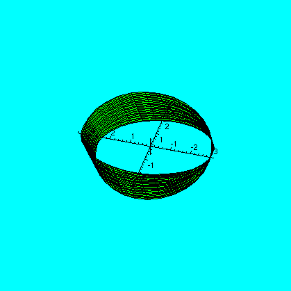
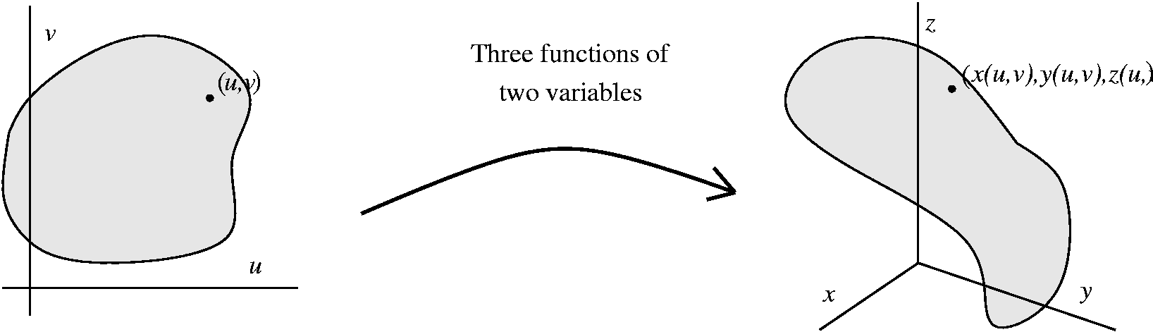
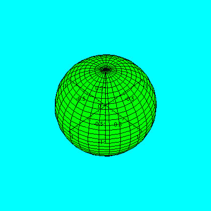
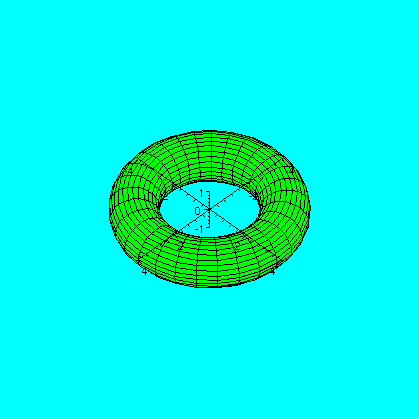
This material uses techniques from almost every part of the course. It can seem conceptually and notationally difficult. It actually is both of those! We started looking again at functions of two variables (to be called u and v) whose ranges were vectors in R3, with components labeled x and y and z. So a vector function P(u,v) would be equal to x(u,v)i+y(u,v)j+z(u,v)k. I rewrote the description of a sphere of radius R and center the origin. Here P(u,v) was R sin v cos ui + R sin v sin uj + R cos vk, where u goes from 0 to 2Pi and v goes from 0 to Pi. This is a description really using spherical coordinates. Then I derived a description of a torus as sketched in the previous lecture (before the exam). Here P(u,v) was (R+r cos v)cos ui + (R+r cos v)sin ui + r sin vk, where both u and v go from 0 to 2Pi. Deriving these formulas was not completely simple! Here Maple is used to draw these parametric surfaces. The sphere has R=1 and the torus has R=3 and r=1.
We then looked at what happened to straight lines in uv-space which went through a point. The partial derivative of P with respect to u, Pu, gave the velocity vector along a curve where only u varied, and v was constant. Similarly, Pv gave a velocity vector along a curve where v varied and u was constant. Each of these vectors was tangent to the surface. Usually the assumption is made that neither vector is a scalar multiple of the other (the velocity vectors are "linearly independent" in the language of linear algebra). This assumption certainly eliminates some simple and silly examples (the "surface" where the function P is constant, for example, or where it depends on only one variable). The assumption also has some other implications which are more intricate to analyze and won't be discussed in this course (for example, "folds" can't occur in such surfaces). It turns out that the tangent plane to the surface is the sum of scalar multiples of these velocity vectors (the collection of all linear combinations of the velocity vectors [the span, again in the language of linear algebra]). The vector PuxPv is always normal to the tangent plane. This tells something about the meaning of the direction of this vector. What about its magnitude? A piece of length along a u-curve was |Pu|du and along a v-curve it was |Pv|dv. Note that these curves need not be perpendicular or orthogonal. The area of a tiny piece of surface (the du by dv rectangle when pushed over into xyz-space by the mapping P is exactly |PuxPv|. That's because the magnitude of the cross product of two vectors is exactly the area formed by the parellelogram determined by these vectors, and the two tiny bits of arc length form (approximately!) the edges of a tiny parellelogram. I tried to draw a picture of this in class but was perhaps not completely successful! I claimed we had at least discussed the following ideas.
We then worked through finding the area of the sphere as a parametric surface. This took some time, effort, and care. When the normal vector was obtained, we checked that it was a scalar multiple of the radius vector, as such vectors are supposed to be for the sphere. We got the correct answer -- at least the answer that we previously had obtained. I neglected to mention that at least in this approach, initially somewhat more intricate, we did not get the intellectually irritating improper integral which we had in the graph approach. We worked through finding the area of the torus. This took further time, effort, and care.After I was done, I "reminded" students about a result called the Theorem of Pappus . (This means I talked a bit about it for the first time for almost all students.) The volume version of the Theorem of Pappus is given at the end of section 8.3 of the text. The area version goes like this: suppose a piece of a curve is revolved about an axis. The surface area which is created is equal to the product of (the length of the curve) and (the distance the center of gravity of the curve piece travels about the axis of rotation). In the case of the tous described here, the two quantities are easy to compute. One is 2PiR and the other is 2Pi(r), so the product is 4Pi2Rr, which is what we got from the parametric surface approach. The "overhead" of initial computations in the parametric approach sometimes seems formidable. It turns out to lead to great insights in many ways, and can really be much superior to the graph approach for analyzing surfaces. This is, for example, mostly the way computer graphics of surfaces is done. I don't have sufficient time to convince students of this. I tried hard to proselytize about it, though.
Word of the day:
proselytize | ||||||||||||||||||||||||||||||||||
| 11/25/2002 |
I discussed some of the fascinating work being done by Professor Wilma
Olson of the Chemistry Department and Professor Bernard
Coleman of the Engineering School, in taking apart pieces of DNA
and investigating their shapes and their uses. I remarked that to
appreciate much of their work, only a rather minimal math background
(several variable calculus and linear algebra) is needed, although the
more biology, chemistry, and physics one knows, the better off one
will be. I strongly suggest that students in this class take advantage
of the wonderful opportunities available for working on very
interesting projects with very intelligent and hard working (and
successful!) people here at Rutgers. I did some more problems from the review sheet and from the textbook in preparation for the exam. Now we returned to surfaces and surface area. Another strategy is actually used by most people who investigate surfaces. Here one takes advantage of "natural" geometric or physical parameters to describe a surface, rather than writing as the graph of a function. This is analogous to the difference between writing the arc length of a curve which is the graph of a function: intabsqrt(1+f'(x)2) dx, and considering the distance traveled by a point whose position is described parametrically: if position is x(t)i+y(t)j, then the length of the path between t=START and t=END is intSTARTENDsqrt(x'(t)2+y'(t)2) dt. We will try to understand what a parametric surface is.
The prototype is a description of a sphere in spherical coordinates. Then (it is conventional to use u and v instead of phi and theta) x(u,v)=R sin(u)cos(v) and y(u,v)=R sin(u)sin(v) and z(u,v)=R cos(u) all describe a sphere with center (0,0,0) and radius R for u in the interval [0,Pi] and v in the interval [0,2Pi]. The lines u=constant are longitudes (?) and the lines v=constant are latitudes. Surfaces can be much more conveniently described this way rather than necessarily as graphs of functions of chunks of the plane.
| ||||||||||||||||||||||||||||||||||
| 11/21/2002 |
| ||||||||||||||||||||||||||||||||||
 We started to work on a description of a torus by
parameterization. The torus consists of circles of radius r, always
in a plane which goes through the z-axis. The centers of these circles
are on a circle of radius R on the xy-plane whose center is the
origin. The problem is to described nice geometric variables which can
be used to "locate" a point on this torus. A pair of such variables
which is frequently used are the following: first, in the small circle
of radius r, use the angle v the point would have with the
xy-plane. Then use the angle u the line connecting the center to the
z-axis makes with the x-axis. This is sort of "spherical
coordinate-like". We can actually get functions by using vector
addition cleverly. The z(u,v) will be z=r sin(v). The other
coordinates will involve both u and v and R and r. We'll finish this
next time.
We started to work on a description of a torus by
parameterization. The torus consists of circles of radius r, always
in a plane which goes through the z-axis. The centers of these circles
are on a circle of radius R on the xy-plane whose center is the
origin. The problem is to described nice geometric variables which can
be used to "locate" a point on this torus. A pair of such variables
which is frequently used are the following: first, in the small circle
of radius r, use the angle v the point would have with the
xy-plane. Then use the angle u the line connecting the center to the
z-axis makes with the x-axis. This is sort of "spherical
coordinate-like". We can actually get functions by using vector
addition cleverly. The z(u,v) will be z=r sin(v). The other
coordinates will involve both u and v and R and r. We'll finish this
next time.
 We simplify a lot in the microscopic view. In addition to making dA
small, we should also assume that dS is almost flat -- in fact, what
the heck, let's assume it is part of a plane. Then by walking "around"
the picture until we see the planar pieces edge on, we can see that
the tilt factor which magnifies the area from dA to dS is just
1/(cos(theta)) where theta is the angle that a vector normal to the
surface (say, a vector N) makes with a vertical vector,
k. So dS=1/(cos(theta)) dA. And cos(theta) can be obtained
as N·k/(||N||) (no length of k necessary
since that is a unit vector).
We simplify a lot in the microscopic view. In addition to making dA
small, we should also assume that dS is almost flat -- in fact, what
the heck, let's assume it is part of a plane. Then by walking "around"
the picture until we see the planar pieces edge on, we can see that
the tilt factor which magnifies the area from dA to dS is just
1/(cos(theta)) where theta is the angle that a vector normal to the
surface (say, a vector N) makes with a vertical vector,
k. So dS=1/(cos(theta)) dA. And cos(theta) can be obtained
as N·k/(||N||) (no length of k necessary
since that is a unit vector).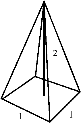
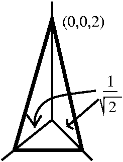 2. I wanted to do another plane, but a tilted (!) one. So I asked for
the area of the tent that was described as follows: the floor of the
tent was a 1-by-1 square. In the center of the tent, a 2 unit pole is
erected, perpendicular to the floor. What area is needed to construct
the lateral walls of the tent? We decided there were 4 walss and we
would look only at one of them. So we put the origin at the center of
the square, and put the half-diagonals of the square along the x and y
axes and the tentpole on the z-axis. Then the sheet of the tent goes
through (0,0,2) and (1/sqrt(2),0,0) and (0,1/sqrt(2),0). The equation
of the plane involved is (sqrt(2))x+(sqrt(2))y+(1/2)z=1, which gives
z=(sqrt(2)/2)x+(sqrt(2)/2)y, and we need to integrate sqrt(17) (that
is what the tilt factor is, and it is a constant) over a right
triangle whose "legs" are 1/sqrt(2) long. This is sqrt(17)/4 and the
total area involved is sqrt(17).
2. I wanted to do another plane, but a tilted (!) one. So I asked for
the area of the tent that was described as follows: the floor of the
tent was a 1-by-1 square. In the center of the tent, a 2 unit pole is
erected, perpendicular to the floor. What area is needed to construct
the lateral walls of the tent? We decided there were 4 walss and we
would look only at one of them. So we put the origin at the center of
the square, and put the half-diagonals of the square along the x and y
axes and the tentpole on the z-axis. Then the sheet of the tent goes
through (0,0,2) and (1/sqrt(2),0,0) and (0,1/sqrt(2),0). The equation
of the plane involved is (sqrt(2))x+(sqrt(2))y+(1/2)z=1, which gives
z=(sqrt(2)/2)x+(sqrt(2)/2)y, and we need to integrate sqrt(17) (that
is what the tilt factor is, and it is a constant) over a right
triangle whose "legs" are 1/sqrt(2) long. This is sqrt(17)/4 and the
total area involved is sqrt(17).