| 10/10/2002
| Ah, well, the last real class before our first exam wasn't a
total disaster but I didn't quite do what I wanted. Let me first tell
what I thought I did, and then comment on what I might additionally
have wished to do.
I summarized looking for extreme values for functions of 1
variable. Here goes:
- A point p in the real numbers is a local
{maximum|minimum} for a
function f if the domain of f includes an interval with p in the
interior of the interval, and if for all x in that interval,
f(x){<|>}=f(p). Now comments about this definition: the
definition really is local. The interval doesn't have to be "big",
just some interval. So if
f(x)=x2-10-100x4 I bet that locally
(near 0) f(x)'s values are positive (the effect of the x4
term is tiny) except that f(0)=0. So 0 is a local min of f. But
certainly when |x| is large, the x4 term dominates, and so
f does not have an absolute min. The word "strict" is sometimes
applied as a modifier to "local" if the = sign is not needed. So the
function f(x)=0 has all local maxes (and mins, actually!) but no
strict local maxes or mins.
- If f is differentiable at a point p, and if f'(p) is not 0, then f
does not have a local max or min at p. That's because from the
definition of differentiability which we reviewed before,
f(p+h)=f(p)+f'(p)h+higher order error. So when h is small, the error
will be much less in absolute value than the f'(p)h term, and that
will make values to the {right|left} bigger than f(p) if f'(p) is
{posi|nega}tive, and values to the {left|right}less that f(p).
- p is a critical point of f if either f'(p) doesn't exist or
f'(p) equals 0. There are lots of "rough" functions where f' doesn't
exist, so that is a possibility which should not be discarded in
practice, although in elementary courses it is frequently
neglected. And finding p's where f'(p)=0 can be difficult with
functions defined by even moderately complicated formulas.
- Local {max|min} must occur at critical points. Examples: |x|,
+/-x2, +/-x3.
- How can one guarantee that a critical point is a local max or min?
A simple "test" uses the second derivative, goes like this: suppose p
has f'(p)=0 (so p is a critical point). Then:
| If | then |
|---|
| f''(p)>0 | p is a local max. |
| f''(p)<0 | p is a local min. |
| f''(p)=0 | no conclusion can be made. |
As for the last line of the table, the examples x3 and
+/-x4 show that the hypotheses can be fulfilled while the
function has no local max or min, or that such a function can
have a local max or min.
- This all really should be thought about in the context of Taylor's
Theorem. This result is very important. If a function f has sufficiently
many derivatives, then
f(p+h)=f(p)+f'(p)h+(f''(p)/2)h2+...+(f(n)(p)/n!)hn+Error(f,p,h,n)
where (the important thing!) the error term --> faster than hn.
This last means precisely that the limit of
Error(f,p,h,n)/hn is 0 as h-->0. Notice that this really looks
like the definition of derivative for the case n=1. Taylor's Theorem
yields "statements" like the 18th derivative test. (?)
This could say something like this: if p is a critical point, and if
f''(p)=f'''(p)=...f(17)(p)=0 and if f18(p) is
not 0, then f has a local max or min at p depending on the sign
of f(18)(p). The reason this is true is that Taylor's Theorem
for n=18 is just (because of all the
ludicrous hypotheses!)
f(p)+(f(18)(p)/18!)h18+Error, and the Error term
is negligible compared to the term immediately before it for |h| small.
I don't know if anyone ever really states such a "test" because it
would hardly ever be used.
How much of all this can be carried over to more than 1 variable? Much
can but some surprises develop, most particularly in the local
geometry of a critical point. Students in 1 variable calc usually
don't like x3 which has an inflection point at 0: the
tangent line crosses the graph. An analogous occurence (the tangent
plane crossing the graph) will occur very often if
n>1. So let's begin.
- A point p in Rn is a local max for a function f if
there is some positive number R so that the domain of f includes all
points at distance <R from p and if x is a point in Rn
with ||x-p||<R then f(x)<=f(p). When n=2, "||x-p||<R" means
points inside a circle of radius R centered at p. When n=3,
"||x-p||<R" means points inside a sphere of radius R centered at p.
For local min just change < to > in what was written.
We had as examples in R4 functions like
f(x)=x1300+5x2600+88x3900+22x46.
Here f(0,0,0,0)=0. Because of the parity (even!) of the exponents and
positivity of the coefficients, f of anything not (0,0,0,0) is
positive. So (0,0,0,0) must be a local min of this f. No other "work"
is necessary! We can of course get a local max by reversing all
the signs. But notice that worse can happen. There are
16=24 choices of signs in this expression. Any of the other
14 choices of sign distribution result in the following behavior:
values of f near (0,0,0,0) which are bigger than 0 and values which
are less than 0. Since grad f at 0 is 0, the tangent plane is
"horizontal" (parallel to the domain plane) and the graph of the
function cuts through it, sort of an inflection behavior. This
behavior is called a saddle point.
- If f is differentiable at p, and if the gradient of f at p is
not 0, then: well, some partial derivative of f at p isn't 0,
so in some "slice" with all varialbes but 1 fixed, we get a function
with non-zero derivative at p, and by the 1 variable analysis above,
in that slice, the functin can't have a local max or min at p. So if
grad f is not 0 at p, p can;'t be a local max or min.
- p is a critical point of f if either f is not
differentiable at p or grad f(p)=0.
- Local {max|min}'s must occur at critical points. We considered
some examples in just two
variables. f(x,y)=sqrt(x2+y2) can be
differentiated from (0,0). grad f is not 0 away from
(0,0). At (0,0) the gradient does not exist (the square root is in the
denominator!) (0,0) is the only critical point, and certainly f(0,0)=0
and f(everywhere else)>0 (just look at the function, don't attempt
to do anything very sophisticated!). Therefore for this function,
(0,0) is a local min (actually an absolute min, in fact). The graph of
this function is a right circular cone, with axis of symmetry the
z-axis and vertex at (0,0,0), a "corner" (it is the graph of |x|
revolved about the z-axis. Then
f(x,y)=+/-x200+/-y300 provides 4 more
examples. This function is differentiable at every point, and the only
critical point is (0,0). For +/+ the c.p. is a local min, for -/- it
is a local max, and for +/- or -/+ it is a saddle point.
Now we'll try to extend a second derivative test to several
variables. This will be complicated. The idea is somehow to use
"second order" information at a critical point to see if the
critical point is a max, a min, or a saddle. Realize, though, that the
test might well "fail" -- that is, it might be inapplicable just as
the 1 variable second derivative test (last line in the table above,
"no conclusion can be made") can also fail.
The simplest situation is 2 variables. Things already get complicated
enough. We try to "bootstrap" from what we already know: that is we
will try to use the second derivative test from one variable to allow
us to get information for two variables.
Here are the starting assumptions: we have a function z=f(x,y) with a
critical point at (a,b). So we know that grad f=0 at (a,b).
If we now "slice"
the graph in R3 of z=f(x,y) by planes perpendicular to the
(x,y)-plane which go through the point (a,b), in each case we get a
curve which has a critical point above (a,b). Let me try to describe
these slices. Choose a two-dimensional direction: that is, a
two-dimensional unit vector. We're lucky that such vectors have a
simple description: u=cos(theta)i+sin(theta)j. A two-dimensional
straight line through (a,b) in the direction of u is just
(a+cos)theta)t,b+sin(theta)t). And f's values on that straight line
are exactly f(a+cos(theta)t,b+sin(theta)t). What's the derivative of
this function with respect to t? We will compute this, but first some
discussion of it: this is the directional derivative of f in the u
direction. It is also the derivative of the curve obtained by slicing
the graph z=f(x,y) by the plane through (a,b,0), perpendicular to the
(x,y)-plane, in the direction of u. So now:
(d/dt)f(a+cos(theta)t,b+sin(theta)t)=
D1f(a+cos(theta)t,b+sin(theta)t)cos(theta)
+D2f(a+cos(theta)t,b+sin(theta)t)sin(theta).
This computation uses the Chain Rule. It is, of course, exactly
Duf, which was defined last time. Since (a,b) is a critical
point, both D1f and D2f are 0 at (a,b). So the
first directional derivative is 0. What we now need to do is take the
t derivative again. We must be careful. Each of
D1f and D2f are functions of 2 variables, and
that each of the two entries in each of these two functions has some
dependence on t: the Chain Rule needs to be used with care. So if we
d/dt what's above (in this
computation theta and a and b are constant), we will get:
d/dt(D1f(a+cos(theta)t,b+sin(theta)t)cos(theta)
+D2f(a+cos(theta)t,b+sin(theta)t)sin(theta))=
D1D1f(a+cos(theta)t,b+sin(theta)t)(cos(theta))2
+D2D1f(a+cos(theta)t,b+sin(theta)t)(cos(theta)sin(theta))
+D1D2f(a+cos(theta)t,b+sin(theta)t)(sin(theta)cos(theta))
+D2D2f(a+cos(theta)t,b+sin(theta)t)(sin(theta))2
and now "plug in" t=0. Remember that cross-partials are equal
(fxy=fyx) and call A=fxx(a,b) and
B=fxy(a,b) and C=fyy(a,b). Then what we have is
A(cos(theta))2+2Bcos(theta)sin(theta)+C(sin(theta))2
We could apply the second derivative test in one variable to this if
we knew appropriate information about every slice. Thus we
could conclude that the critical point (a,b) was a minimum if for
every theta, the expression above was positive. If theta=0 this means
that A=fxx(a,b) should be positive. But even more needs to
be true. Suppose we divide the expression above by
(cos(theta))2 and we call w=tan(theta) (this is
weird!). Then what is written above is just
A+2Bw+Cw2 and we would like to know what
conditions on A and B and C would imply that this is always
positive. We did something like this in the lecture 9/9. This
positivity will occur exactly when the quadratic has no real reals. So
(2B)2-4AC should be negative. (The parabola
A+2Bw+Cw2 will then never intersect the w-axis and since
A>0 it must always be positive.!)
This somewhat subtle reasoning leads to what is called the Second
Derivative Test for
functions of two variables. First, define the Hessian, H, to be
      | fxx  fxy |
H=det |          |
      | fxy  fyy |
and
suppose that (a,b) is a critical point of f.
| If | and if | then |
|---|
| H(a,b)>0 | fxx(a,b)>0 | p is a local max. |
| fxx(a,b)<0 | p is a local min. |
| H(a,b)<0 | p is a saddle point. |
| H(a,b)=0 | no conclusion can be made. |
This statement needs examples. But it does
display the local "structure" of a critical point a bit. (I
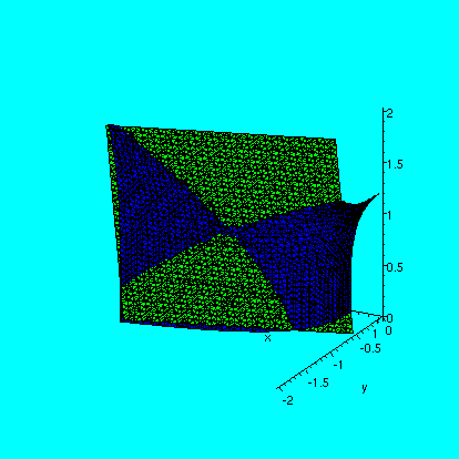
very briefly looked at f(x,y)=xy.)
Please do some problems in section 14.7.
This should give you some idea of the complexity of critical point
behavior in more than 1 variable. Although much is known already, this
is actually an object of current research. |
| 10/9/2002
| I finally got around to something I should have discussed
several lectures ago. First, a mean thing done to Maple: I
typed z:=x^2*arctan(y*exp(y)); and then I asked
Maple to compute diff(diff(z,y$30),x$3); which is
the 30th derivative with respect to y of z followed by 3
derivatives with respect to x. The result was 0, and the computation
time needed was 5.539 seconds on the PC in my office. Of course what
Maple did was compute 30 derivatives of a complicated
function, and these derivatives get very big in terms of data
(this is called "expression swell"), and take time and storage space
to manipulate. Then there were 3 x derivatives, and the result was
0. On the other hand, when I instructed Maple to do the x
derivatives first and then the y derivatives, the program reported no
elapsed time used (that means, less than a thousandth of a
second).
What's going on? The result needed here is called in your text
Clairaut's Theorem, and loosely states that the order of taking "mixed"
partial derivatives (derivatives with respect to different variables)
doesn't matter. More precisely, the result is: if f is a function of
two variables, x and y, and if both fxy and fyx
exist and are continuous, then they must be equal. I tried to
motivate this with a brief allusion to spreadsheets (!) and then
remarked that an actual proof is in appendix F of the text, and
uses the Mean Value Theorem 4 times, in much the same manner as we've
already seen (the lecture on 10/3). I didn't have the time or desire
to give the proof.
Here, though, is an example to show that some hypotheses are needed to
guarantee the equality of the mixed partials:
| A function f with fxy NOT equal to
fyx |
PDF
Picture |
The main topic of today's class was flying a rocket ship. Suppose we
have a rocket ship flying through a nebula. The nebula is a cloud of
matter, with qualities such as pressure and temperature. So I decided
to consider the temperature. What contributes to the temperature of
the nebula as perceived by the crew of the rocket ship? An analysis of
this question mathematically using the tools we already have is
possible if we describe everything algebraically. So suppose the
flight path of the rocket ship is given as a parametric curve. That
is, x=x(t), y=y(t), and z=z(t). This is the same as giving a position
vector, R(t)=x(t)i+y(t)j+z(t)k. We know about this, and about the
first and second derivatives of position (which are velocity and
acceleration, respectively). The temperature depends on the location
in the nebula, so that is a function T of (x,y,z), the coordinates of
a point in the nebula: usually we write T(x,y,z).
The temperature of the point in the nebula outside the rocket ship at
time t is T(x(t),y(t), z(t)). How does the temperature change? This
is, of course,
(d/dt)T=Tx(dx/dt)+Ty(dy/dt)+Tz(dz/dt).
Some contemplation of this formula allows a certain "decoupling" to
take place, that is, a separation of the influence of the rocket ship
and of the temperature. We recognize that the velocity vector is
V(t)=(dx/dt)i+(dy/dt)j+(dz/dt)k. And then we see that (d/dt)T is
really a dot product of V(t) with another vector, namely
Txi+Tyj+Tzk. This vector is called
the gradient of T, written sometimes as (upside down triangle)T and
sometimes called grad T. I'll call it grad T here because of
typographical limitations.
There were some questions about grad T, so I invented a rather simple
example, something like the following: if
T(x,y,z)=3x2+4xy3+z4, then
T(2,-1,1)=5. And grad T=6xi+12xy2+4z3. At
p=(2,-1,2), grad T is 12i+24j+4k. grad T is a vector function
of position, while T itself is a scalar function.
Then (d/dt)T turns out to be the dot product of grad T with V(t).
Observation 1 We have separated the effects of temperature and
the rocket. In fact, all that matters in the computation of (d/dt)T
from the rocket is the velocity. If two rocket ships go through the
same point with the same velocities, then (d/dt)T will be the
same. All that matters is the velocity: the tangent direction to the
flight path (a curve) and the speed (the lenght of V).
Observation 2 How can we make (d/dt)T big? If it isn't 0, we
could always make the rocket ship move faster. If we increase the
speed by a factor of M>0, then (d/dt)T will multiply by M. This is
because (d/dt)T is ||V|| ||grad T|| cos(angle between V and
grad T). Multiplication of V by M results in a multiplication of ||V||
by M, and nothing else changes. So (d/dt)T gets bigger.
Observation 3 But really the answer to the previous question
was a bit silly. We should try to look at different directions. What
direction will cause the derivative to be larger? So we defined the
directional derivative of T with respect to a unit vector u:
DuT. This was the rate of change of T with respect to a
"rocket ship" moving with unit speed in the direction of u, and it is
just u· grad T. Since this is ||u|| ||grad T|| cos(angle
between them) and we've restricted ||u|| to be a unit vector, we see
the only ingredient we've got to vary is the angle. Indeed,
immediately we have: The directional derivative is always
between -||grad T|| and ||grad T||. This is because cosine's
values are in [-1,1]. More is true, when grad T is not the 0 vector.
The unique unit vector maximizing the directional derivative
is (grad T)/||grad T||. The unique unit vector
minimizing the directional derivative is -(grad T)/||grad
T||. This turns out to have many computational
implications.
I went back to the example and found the directional
derivative of that T in various directions, including the maximizing
direction and the minimizing one.
Observation 4 Isothermals are collections of points where the
temperature is constant. If T(2,-1,1) is 5, then (2,-1,1) is in the
isothermal (the level set) associated to the temperature 5. If the
rocket ship flies in an isothermal, then the rate of change of the
temperature perceived by the rocket ship is 0. So (d/dt)T=0 and by the
decoupling we've already seen, that means V(t)·grad T=0. So the
velocity vector of such a flight is always perpendicular (normal) to
the gradient vector. From this evidence and the knowledge that grad T
at (2,-1,1) is 12i+24j+4k we were able to deduce that the plane
tangent to the surface T(x,y,z)=9 is
12(x-2)+24(z+1)+4(z-1)=0. Directions normal to the gradient have zero
first order change.
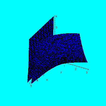
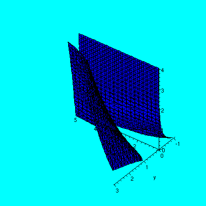
Here is a command to graph a chunk of the surface T(x,y,z)=5 and store
the graph in the variable A:
A:=implicitplot3d(3*x^2+4*x*y^3+z^4=5,x=1..3,y=-2..0,z=0..2,
grid=[40,40,40],axes=normal,color=green):
Here is a command to graph and store as a variable B a piece
of the candidate for the tangent plane which we computed:
B:=implicitplot3d(8*(x-2)+24*(y+1)+4*(z-1)=0,x=1..3,y=-2..0,z=0..2,
grid=[40,40,40],axes=normal,color=red):
And finally the command display3d(A,B) displays both graphs
together. The result is shown below. Note that the tangent plane
actually cuts through the surface (a saddle-more about this next
time!).
 Then I discussed how people might want to computationally maximize
("hill climbing") or minimize ("method of steepest descent") functions
of many variables. To increase (respectively decrease) a function W of
many variables, compute grad W, and move in the direction of grad W
(respectively - grad W) "for a while". Then repeat (because the
direction of grad W will likely change). There are many technicalities
in all this: how big are the steps to move, and when should one
terminate the procedure. Answers to these questions may depend on
the specific nature of the functions and the situations. I looked at a
specific function of 4 variables (I think it was
p2exp(q-rs) and computed its (4-dimensional) gradient at
(2,1,-2,1).
Then I discussed how people might want to computationally maximize
("hill climbing") or minimize ("method of steepest descent") functions
of many variables. To increase (respectively decrease) a function W of
many variables, compute grad W, and move in the direction of grad W
(respectively - grad W) "for a while". Then repeat (because the
direction of grad W will likely change). There are many technicalities
in all this: how big are the steps to move, and when should one
terminate the procedure. Answers to these questions may depend on
the specific nature of the functions and the situations. I looked at a
specific function of 4 variables (I think it was
p2exp(q-rs) and computed its (4-dimensional) gradient at
(2,1,-2,1).
I sketched some level curves for the function
10-2x2-y2 and related the gradient of the
function to the level curves: again the gradient is perpendicular to
the level curves, and points in the direction of increasing function
value.
I gave out and discussed the review problems.
|
| 10/3/2002
| A function of one variable, f(x), is differentiable if
f(x+h) can be written in the following way:
f(x+h)=f(x)+Ah+Error(f,x,h)h
where: 1) A is a number not depending on h but possibly depending on x
and f (A is called f'(x) usually); 2) Error(f,x,h)-->0 as h-->0.
Parenthetical remark: I mentioned that if we knew a function of 1
variable was equal to its Taylor series, then the error term could be
written as a sum of an infinite tail of the series, so that's what
"Error" could be. Of course, many functions don't have a Taylor series
and/or don't have a readily computable Taylor series, so the value of
that observation is unclear!
I want to define something similar for functions of two
variables. Preliminarily, f(x,y) will be differentiable if
f(x+h,y+k) can be written in the following way:
f(x+h,y+k)=f(x,y)+Ah+Bk+Error1(f,x,y,h,k)h+Error2(f,x,y,h,k)k
where Error1 and Error2 both -->0 as
(h,k)-->(0,0).
This is a complicated statement and needs some investigation. First,
the equation is true for any selections of h and k. So we can look at
any special values we care to. For example, if k=0 and h is not 0, we
can rewrite the equation to become
((f(x+h,y)-f(x,y))/h)=A+Error1. But as h-->0, the
right-hand side-->A (since the Error terms go to 0). That means the
left-hand side has a limit. So if f is differentiable, then
fx exists and equals A. Similarly (set h=0 and let k-->0)
if f is differentiable, then fy exists and is B. Therefore,
If f is differentiable, the partial derivatives of f
exist.
The converse of that statement is generally not true.
The
converse of a simple implication reverses the hypothesis and
the conclusion. For example, the converse of "If Fred is a frog, then
Fred hops" is "If Fred hops, then Fred is a frog." Even this simple a
statement shows that a converse need not be true.
The function we looked at last time, defined by
f(x,y)=(xy)/sqrt(x2+y2) if (x,y) is not (0,0)
and by 0 if x and y are both 0 has some interesting properties. First,
f has partial derivatives at every point. Why? Away from (0,0), the partial
derivatives can be computed by the standard algorithms of 1-variable
calculus. At (0,0), we notice that f is 0 on both the x and y axes, so
the partials both exist and are 0. But consider f(w,w) where w is a
small positive number. Direct computation in the formula shows that
f(w,w,) is (1/sqrt(2))w. But if f were differentiable at (0,0) the
wonderfully complicated definition above would apply. The right-hand
side of the formula is
f(x,y)+fx(0,0)h+fy(0,0)k+Error1(f,x,y,h,k)h+Error2(f,x,y,h,k)k
but f(0,0) and fx(0,0) and fy(0,0) are all 0. So
f(w,w)=Error1(f,x,y,w,w)w+Error2(f,x,y,w,w)w.
If we remember that f(w,w) is (1/sqrt(2))w and divide the equation by
w, we get (1/sqrt(2))=Error1+Error2 and both of
the errors-->0 as w-->0. So the right-hand side-->0 but the left-hand side
does not. This rather intricate contradiction shows that this f is
not differentiable at (0,0).
Several things still may not (probably are not!) clear to a
student right now. What are the reasons for defining "differentiable"
in this intricate manner? How could one check that
specific functions defined by formulas are differentiable?
Here is one answer to the second question. The first will be answered
several times during the rest of this course. Suppose we want to
compare f(x+h, y+k) and f(x,y). Then consider:
f(x+h,y+k)-f(x,y)=f(x+h,y+k)+0-f(x,y)=f(x+h,y+k)-f(x,y+k)+f(x,y+k)-f(x,y).
We have again written a 2-variable change as a succession of
1-variable changes.
The 1-variable Mean Value Theorem shows that
f(x,y+k)-f(x,y)=fy(x,y+betak)k where
|betak|<|k|. Also
f(x+h,y+k)-f(x,y+k)=fx(x+alphah,y+k)k where
|alphah|<|h|. Here's the big hypothesis coming:
if the partial derivatives are continuous, then the difference between
fy(x,y+betak) and fy(x,y) approaches
0 as k-->0. And the difference between
fx(x+alphah,y+k) and fx(x,y) also
goes to 0 as (h,k)-->(0,0). These differences both get put into the
error terms, and so we see
If the partial derivatives are continuous, then the function
is differentiable.
The contrast between differentiability and partial derivatives doesn't
really have a good analogy in 1 variable: it seemed new to me when I
first saw it and I needed time and effort to understand it. There
are some further examples to illustrate the complicated logical
relationships from a calculus course at MIT:
| A function f so that fx and fy exist
everywhere, but f is NOT differentiable |
PDF
Picture |
| A function f which is differentiable although fx and
fy are NOT continuous |
PDF
Picture |
In this course, almost all the functions will be defined by formulas
and the formulas can be differentiated, and, inside usually easily
defined domains, the partial derivatives will be continuous, so the
functions will be differentiable.
Then I went through problem #19 of section 14.4, a rather
straightforward application of the linear approximation (that's the
constant term plus the first degree terms) to an incremented value of
the function. The numbers worked out nicely, and, in this example, the
errors were fairly small.
I concluded by finding a tangent plane to a graph, I think the graph
of z=5x2+2y4, a sort of a cup, at the point
(2,1,22). I did this by examining the section of the graph where
y=1. This gives a curve with equation z=5x2+2 whose
derivative at (2,22) was 10x, or 20. Therefore 1i+0j+20k was tangent
to the surface at (2,1,22). A similar analysis when x=2 shows that
0i+1j+8k was also tangent to the surface at that point. Therefore the
cross product of these vectors would be perpendicular to the tangent
plane. We computed the cross-product and it was -20i-8j+k (generally
it will be -fxi-fyj+k) and the plane went
through the point (2,1,22), so the desired tangent line is
-20(x-2)-8(y-1)+(z-22)=0.
I remarked that on an exam I would rather not have such an
answer "simplified" which brought up the question of
Exam conditions and schedule
- I'd like to give the first exam after we finish 14.5, 14.6,
and 14.7, as planned on the schedule. I would also give out review
material. So I tentatively would like to give the exam on Wednesday,
October 16.
- I would like to eliminate time pressure on the exam, so I will try
to get a room we can stay in for more than the standard period (more
than 4:30--5:50). I will not use this as a reason to make an
exam long or excessively difficult.
- I will try to schedule a review session on Tuesday evening,
October 15.
- My feeling right now is that calculator use should be minimal on
an exam in this course. I would like to restrict the use of
calculators to the last 20 minutes of an exam.
- Some of the formulas may seem intricate to you (to me, too!). I would be happy
to write a formula sheet which would be attached to the exam. Please
let me know what
formulas that you believe you will need.
|
| 10/2/2002
| Matthew Gurkovich presented a solution to problem 3 in
workshop 3. I thank him for this. I think the most difficult part of
this problem is recognizing that the letter "t" serves two different
purposes in the problem.
I analyzed the idea of differentiability for functions of 1
variable. What is the derivative? Some ideas are i) rate of change,
ii) slope of the tangent line to the graph of the function, iii) a
certain limit, and iv) velocity or acceleration. And certainly there
are others.
As a limit, f'(x)=limh-->0(f(x+h)-f(x))/h. Of course this
limit is paradoxical contrast to the basic "limit reason" for looking
at continuous functions: those limits can be evaluated just by
"plugging in", and here such an approach results in the forbidden
0/0.
Removal of the "limh-->" prefix to the defining equation
above yields a statement which is generally false: there is an error
involved. Also the division and minus signs are a complicating
feature. So we transform the equation above into the following:
f(x+h)=f(x)+f'(x)h+Error(f,x,h)h
where Error(f,x,h) is something (possibly [probably!]) very
complicated depending on f and x and h with the property that (with f
and x held fixed) that Error(f,x,h)-->0 as h-->0. With perspective
that further study of calculus gives, we know that if f is equal to
its Taylor series, then the Error(f,x,h)h is just a sum of terms
involving powers of h higher than 1, so at least one power of h can be
factored out. The result is something that goes to 0 "faster" than h:
order higher than first order. So a perturbation in the argument, x,
to a function f(x), that is, x changes to x+h (h may be either
positive or negative) yields f(x)+f'(x)h+Error(f,x,h)h. The first term
is the old valuye, the second term is directly proportional to the
change, h, with constant of proportionality f'(x), while the third
term -->0 with more than first order in h.
In particular, this shows easily that if h-->0 then f(x+h)-->f(x), so
differentiable functions (which are those having such a
"decomposition") must be continuous. But more than continuity is
involved. The simple example
      2x if x>0
f(x)= 0 if x=0
     (-1/3)x if x<0
shows that the same multiplier is needed on
both sides of 0: 2 can't be deformed into -1/3 by concealing
things in the error term. So this function is not
differentiable.
The aim is to define a similar "good" decomposition for functions of
more than 1 variable: (old value)+(linear or first order
change)+(error of higher order)
Now I looked at 2 variable functions. I defined fx, the
partial derivative with respect to x, as the limit as h-->0 of
(f(x+h,y)-f(x,y))/h, and fy, the
partial derivative with respect to y, as the limit as k-->0 of
(f(x,y+k)-f(x,y))/k, if either or both of these limits
exist. The choice of letters (k and h) are conventional,
and of course we could use anything.
We computed some partial derivatives for functions which looked like
5x2y5 and xexy2 and
arctan(y/x). The routine differentiation algorithms (rules for
derivatives) work here.
More suspicious examples were considered. The first is f(x,y)=0 if
xy=0 and 1 otherwise. This function had the following properties: away
from the coordinate axes (where xy=0) both fx and
fy are 0. On the y-axis, fy is 0 and on the
x-axis, fx is 0. At (0,0), both fx and
fy exist and are 0. The limits for the other partial
derivatives don't exist. But notice that f(0+h,0+k) compared to
f(0,0)+fx(0,0)h+fy(0,0)k+ERROR where somehow ERROR should go to 0 faster than first
order. But that means f(h,k)=(three zero terms)+ERROR. Since if both h and k are small
positive numbers, we get 1=ERROR,
apparently the decomposition is impossible! So (when the
correct definition is given!) this f has partial derivatives at (0,0)
but is not differentiable at (0,0)!
Then I looked at the function f(x,y)=r cos theta sin theta
with x and y in polar coordinates. A more mysterious formula for
f(x,y) results if we use x=r cos theta and y=r sin theta:
f(x,y)=(xy)/sqrt(x2+y2). The graph of this
function includes the x and y axes: f's values are zero there. But
then the partial derivatives of f at (0,0) both must exist and are
0. But f(w,w)=.5w, so the change along the line y=x is certainly first
order, but cannot be accounted for in the formula
f(x+h,y+k)=f(x,y)+Ah+Bk+ERROR. If we take k=0, then a limit
manipulation shows that A must be fx(x,y) and
B must be fy(x,y). For this function, both partial
derivatives exist at all points, and both are 0 at (0,0). Therefore
f(0+h,0+k)=0+0+0+ERROR. But f(w,w) is .5w=ERROR, and the right-hand side is higher than
first order as w-->0 and the left-hand side is not. More will follow
about this tomorrow.
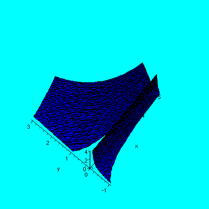
Here's the result of the Maple command
plot3d((x*y)/sqrt(x^2+y^2),x=-3..3,y=-3..3,grid=[30,30],axes=normal,color=pink);
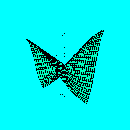 and
maybe the picture will help you understand the properties of the
function. The colors seem fairly unreliable!
and
maybe the picture will help you understand the properties of the
function. The colors seem fairly unreliable!
|
| 9/30/2002
| I began by considering how continuity is defined. In one
variable, a function f is continuous at x0 if
limx-->x0 f(x)
exists and equals f(x0). Combining this with the official
definition of limit given last time, we see:
| Definition of continuity |
A function f is continuous at x0 if, given any eps>0, there
is a delta>0 so that
if |x-x0|<delta,
then |f(x)-f(x0)|<eps.
|
The definition says that limits can be evaluated in the simplest
possible fashion, just by "plugging in". It is an important
definition which I wanted to work with.
First we looked at the function n(x,y), defined last time. I asked
where n was continuous: that is, for which
(x0,y0) does the limit of
n(x,y) as (x,y)-->(x0,y0) exist and is it equal to
n(x0,y0)?
First we approached the question "emotionally": where is n
continuous? After some discussion, it was decided that n would be
continuous "off" the parabola, that is, for
(x0,y0) where y0 is
not equal to (x0)2. Away from the parabola, the
graph of the function is quite flat (always 0). So if (x,y) is close
enough, then n(x,y) is really 0 around
(x0,y0). So it should be continuous. If
(x0,y0) is on the parabola, though, the limit
won't exist.
I then said that I wanted to work with the definition, and verify
that: n(x,y) is continuous at (0,1) and n(x,y) is not
continuous at (0,0).
How to verify that n(x,y) is continuous at (0,1): if we take delta to
be, say, 1/2, then ||(a,b)-(0,1)||<1/2 means that (a,b) is
not on the parabola (the 1/2 is actually chosen for this
reason!), so that n(a,b)=0 and n(0,1)=0 also, and therefore
|n(a,b)-n(0,1)|<eps for any positive eps.
The choice of delta here is rather easy and almost straightforward. In
general, the choice of delta likely will depend on
(x0,y0) and on eps.
Then we went on to try to show that n is not continuous at
(0,0). Here we need to verify the negation of the continuity
statement. Negations of complicated logical statements can be quite
annoying to state. In this case, we need to do the following:
| Negation of continuity |
| There is at least one eps>0 so that for all delta>0
there is an (a,b) in R2 with
||(a,b)-(x0,y0)||<delta and
|n(a,b)-n(x0,y0)|>eps.
|
Here (x0,y0) is (0,0) and n(0,0)=1. The values
of n(a,b) are either 0 or 1 (n is actually a rather simple
function!). So we guess that a useful eps to try will be 1/2. Then
to get |n(a,b)-n(x0,y0)| at least 1/2 we'd
better have n(a,b) equal to 0. That means (a,b) should be off the
parabola. So we need (a,b) off the parabola and also within distance
delta of (0,0). The suggestion was made that we take (a,b) to be
(0,delta/2), and this does work. Note that the (a,b) varies with the
delta.
What are the simplest functions usually considered to be continuous>
Thank goodness the suggestion was made that polynomials are continuous
because I had prepared
an analysis of the continuity of the polynomial
f(x,y,z)=x2y2-4yz. We expect that this
polynomial (and, indeed, all polynomials) are actually
continuous at every point. So the limits should be evaluated just by
"plugging in". In fact, the limit of f(x,y,z) as (x,y,z)-->(3,1,2)
should just be f(3,1,2) which is 1.
I verified the definition for this limit statement. The verification
used entirely elementary methods, but was quite intricate is spite of
that.
We looked at:
|f(x,y,z)-1|=|x2y2-4yz-1|=|(x2y2-4yz)-(3212-4·1·2)|.
Then
the triangle inequality was used, so that the last term is less than
or equal to
|x2y2-3212|+|-4yz+4·1·2|.
The second of these expressions seems a bit easier to handle, so:
|-4yz+4·1·2|<|4|·|yz-1·2|. Here I tried
to suggest that too much was changing. This is handled by making
the difference equal to several one variable differences. So:
|4|·|yz-1·2|=4|yz + 0 -1·2|=
4|yz-y2+y2-1·2|=4(|(yz-y2)+(y2-1·2)|). And again split
up by the triangle inequality: 4|yz-y2|+4|y2-1·2|. The second
term looks easiest to handle.
Get a "bound" on 4|y2-1·2|=8|y-1| by making |y-1| sufficiently
small. Since we had split up the original difference into two parts
and then split the part we were considering into two parts, I guessed
that it would be good enough to make this less than eps/4. So we would
need |y-1|<eps/32.
Now we considered 4|yz-y2|=4|y|·|z-2|. To get this less than
eps/4 we would make |z-2| small. But to control the product we needed
to control the size of |y|. Well, if (pulled out of the air!)
|y-1|<1 then I knew that
0<y<2, so |y|<2. Therefore
4|y|·|z-2|<4·2·|z-2|. This will be less than
eps/4 if |z-2|<eps/32. As I
mentioned in class, the coincidence of the 32's made me uneasy.
Now we are half done. We still need to estimate the difference:
|x2y2-3212|. Again we
write it as a succession of differences of one variable:
|x2y2-3212|=|x2y2-x212+x212-3212|.
And again the triangle inequality leaves us with estimation of two
pieces:|x2y2-x212| and
|x212-3212|.
We do the second part first.
|x212-3212|=|x2-32|=|x+3|·|x-3|.
If, say, |x-3|<1 then x is between 2
and 4 so |x+3| is between 5 and 7, and therefore
|x2-32|=|x+3|·|x-3|<7|x-3|. This will
be less than eps/4 if we require |x-3|<eps/28. (Somehow the numbers came out
differently in class!)
The final piece to handle is
|x2y2-x212|=|x2|·|y-1|.
Since we have already controlled |x| (it is less than 4) we know
that |x2| is less than 16. Therefore
|x2|·|y-1|<16|y-1|. This will be less than eps/4
if we require |y-1|<eps/64
If we collect all the restrictions on the variables, we see that the
implication
"if ||(x,y,z,)-(3,1,2)||<delta then |f(x,y,z)-f(3,1,2)|<eps"
will be true when delta is chosen to be the minimum of all the
blue restrictions. Therefore choose
delta to be the minimum of 1, eps/32, eps/28, and eps/64.
The technique I outlined is a bit painful, but it does work and it is
"elementary".
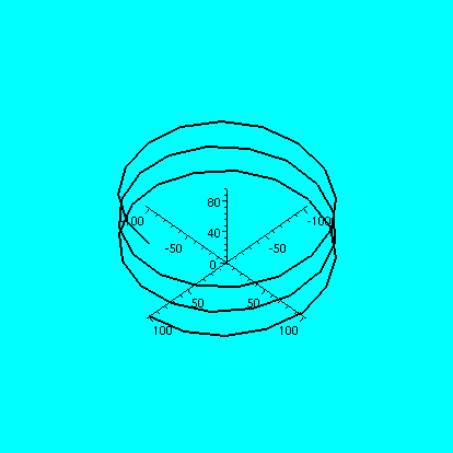
A picture of what f(x,y,z) looks like doesn't seem to
help very much. Here, for example, are three views of the output of
the Maple command
implicitplot3d(x^2*y^2-4*y*z=1,x=1..8,y=-1..3,z=-2..4,grid=[20,20,20],
color=green,axes=normal);.
The procedure implicitplot3d is loaded by
with(plots); and plots implicitly defined surfaces, just as
implicitplot itself plots implicitly defined curves. The
option grid=[20,20,20] alters the sampling rate
Maple uses. The default is [10,10,10], which makes quite a
rough picture. On the other hand, one can ask for [50,50,50] which
will take about 125 (53) as much time as the default. I
just experimented at home. Sketching a sphere with the default grid took
.070 seconds, and the [50,50,50] grid took 7.719 seconds. Indeed: in
practical applications, the tradeoff between time and picture detail
can be interesting.
Pictures of f(x,y,z)=1=f(3,1,2)
 |
 |
 |
| x-axis pointing "out" |
y-axis pointing "out" |
z-axis pointing "out" |
I then discussed workload in the course.
- I expected that students would spend 10 to 12 hours per week
outside of class on the course, doing workshop problems and the
textbook homework problems.
- The workshop problems should be done neatly, with the pages
fastened (stapled or with paperclips), with complete English
sentences, with details of computations only indicated and not given.
- Students could hand in do-overs of one workshop problem per
workshop. These writeups would need to be done individually. Other
students could be consulted, but the writeups themselves would need to
be done individually. These redone workshop problems would be due on
Wednesday, October 2.
- I invited students to give oral presentations (5 points per
problem bonus) of problems 3 and 4 and 5 of workshop #3, at most 5
minutes per problem, at the beginning of class on Wednesday. Please
send me e-mail if you want to do this. I hope
that by the end of the semester every student would have presented at
least one problem to the class.
|
| 9/26/2002
| The instructor rudely began by filling some boards with
remarks about limits and continuity in 1 dimension. Consider
f(x)=x2. A sketch was drawn. What happens to f(x) as x-->4?
Clearly limx-->4x2=16. What does this mean?
This is a limit statement, and the official definition of limit is as
follows:limx-->af(x)=b means given any eps>0 there is a delta>0 so that
if 0<|x-a|<delta, then |f(x)-b|<eps.
(This is in bold because it is important in the history and theory of the subject!)
Here due to the limitations of html, "eps" will be written in place of
the usually used Greek letter "epsilon" and "delta", in place of
the usually used Greek letter "delta".
Here this means: given eps>0, find delta>0 so that if
|x-4|<delta, then |x2-4|<eps. In order to verify that
this implication is correct, some connection between |x-4| and
|x2-16|. But in fact |x2-16|=|x-4| |x+4|.
In order to really be convinced that this is true, we need to show
that when |x-4| is small, |x+4| is controlled. That is, it does no
good to verify that a product of two factors is small by showing that
one factor of a product is small, if the size of the other product
can't be controlled.
Here is a small "computation": if |x-4|<1, then -1<x-4<1, so
3<x<5 so that 7<x+4<9 and consequently |x+4|<9. Now we
can do the proof.
| The official proof |
Suppose eps>0. Take delta to be the smaller of 1 and eps/9. Then if
|x-4|<delta, |x2-16|=|x-4| |x+4|<(eps/9)9. The
inequality |x-4|<eps/9 follows from the definition of delta. The
inequality |x+4|<9 follows from the other part of the definition of
delta followed by the "computation" above. Therefore
|x2-16|<eps, and the limit statement is proved.
|
The relevance of the official definition of limit to real people in
real life is maybe not too clear. First, revealing the official
definition is an effort to encourage people not to interpret the limit
statement as just "plugging in" a for x in a formula for f(x) (that's
what we like to do, and in fact we do it for well-behaved functions --
exactly the continuous functions. The other observation is that
the eps-delta connection is relevant in more detailed analyses of
functions, where one tries to relate the "output tolerance" for an
error (how close to f(b) are we?) to the input tolerance for error
(how close to a need we be to produce at most an appropriate error in
the output?).
Then I began analyzing functions in R2. We began by looking
at f(x,y)=x2+y2. I drew a graph of this: the
graph was a collection of points in R3. I also commented on
the contour lines. I strongly recommended the Maple
procedures plot3d and contourplot and
contourplot3d. You need to type the command
with(plots); before using these procedures.
| Maple command followed by a picture of
its output |
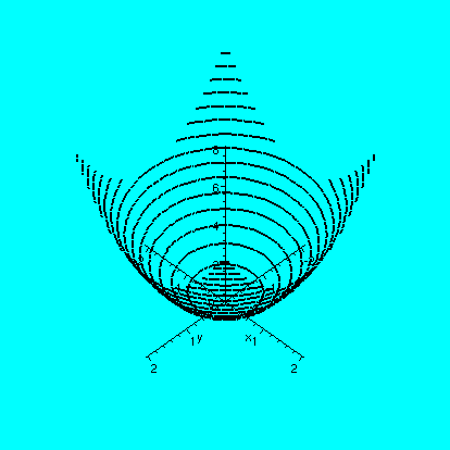
plot3d(x^2+y^2,x=-2..2,y=-2..2,axes=normal);
 |
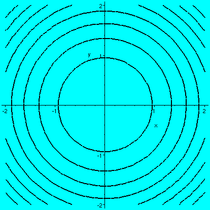
contourplot(x^2+y^2,x=-2..2,y=-2..2,axes=normal,color=black,thickness=2);
|
contourplot3d(x^2+y^2,x=-2..2,y=-2..2,axes=normal,color=black,thickness=2);
|
Functions defined by such simple formulas will be continuous, so
lim(x,y)-->(x0,y0)x2+y2=(x0)2+(y0)2
"naturally". In fact a detailed verification is much like what I just
did in one variable. I would like to concentrate on aspects of limit
and continuity which are somewhat new because of more than 1
variable.
We considered the function g(x,y) defined piecewise by g(x,y)=1 if
(x,y) is NOT (0,0) and which is 0 if (x,y)=(0,0). The graph is a plane
parallel to the (x,y)-plane, 1 unit "up" in the z direction, except
for the origin, which is back at (0,0,0). I asked when the limit as
(x,y)-->(x0,y0) existed and what the value
was. Some discussion followed, and the somewhat disconcerting truth
was told: the limit always exists and it always is 1. This example can
be done in one variable, though.
The piecewise function h(x,y) defined by = 1 if x>0
h(x,y)=37 if x=0
= 2 if x<0has
lim(x,y)-->(x0,y0)h(x,y)
existing if x is NOT 0, and for x0>0 the limit is 1
while for x0<0 the limit is 2.
A much more subtle example is provided by
m(x,y)=(x2-y2)/(x2+y2).
This function is "fine" (continuous) away from (0,0). The limit along
rays through the origin varies with the ray. Along the positive and
negative x-axis the limit is 1, but along the positive and negative
y-axis the limit is -1. Along y=Mx, the limit is
(1-M2)/(1+M2). I tried to show this surface with
a demonstration in class. It is interesting to view the surface using
Maple. The procedure contourplot3d gave the "best"
picture for me.
I finally looked at n(x,y). This is peculiar piecewise-defined
function. Its value is 1 if y=x2 and 0 otherwise. It has
the property that limits along any straight line through (0,0)
exist, and all these limits are 0 BUT the limit as (x,y)-->(0,0) does
NOT exist. I tried to explain this.
The text gives an example of a rational function:
(xy2)/(x2+y4) (see p.890 in section
14.2) with similar properties, which maybe is harder to
understand.
As a pop quiz, I asked students to create a function so that the limit
as (x,y)-->(x0,y0) did not exist if
x2+y2=1 but did exist for all other (x,y). I
urged students to begin reading chapter 14.
|
| 9/25/2002
| Hardly any "progress" was made. We did more and more problems
from chapter 13. Attempts were made by valiant students to really get
me to explain what CURVATURE and TORSION:
Google reports only about 16,700 links with
information about both of these.
Curvature, I tried to insist, referred to how much a curve bends. I
gave another interpretation using the idea of the osculating
circle. If a circle agrees "up to second order" (passes through a
point, and first and second derivatives agree) with the graph of a
function, then 1/(the radius of the circle) turns out to be the
curvature. The circle is called the osculating circle. My online
dictionary states:1. [Math.] (of a curve or surface) have contact of at least the second
order with; have two branches with a common tangent, with each branch
extending in both directions of the tangent.
2. v.intr. & tr. kiss. The osculating circle is a second
order analog of a tangent line. The tangent line agrees with a curve
up to first
order (value and first derivative of the curve and tangent line should
agree). The osculating circle does the same up to second order.
So where the closest circle is
small, the curve bends a lot.
Torsion is weirder. In a picture on this link an
attempt is being made to show "high torsion when there is
rapid departure from a plane."
In my Google search I found web pages dealing with
the relationship of curvature and torsion to
coronary arteries and blood flow, concrete, plasma flow, how birds and
gnats and
flies fly,
"carbon nanotubes" (thin filaments),
models of molecules, motion of robots and octopuses and
cilia and flagella ... and so on. I found Maple routines for
computation of curvature and torsion: lots of stuff, most of it
quite technical in both its applications and its mathematics. Lots of
stuff! I tried to argue that Problem #5 on Workshop #3 showed that
curvature could be concealed easily. According to Einstein, "the Lord
is subtle but not mean" (approximately) and that knowing that the
structure of a curve means dealing with its curvature and
torsion sometimes may make life easier. Problem #5 has exquisitely
disguised simple curves: in a), a circle, and in b), a straight
line.
The next few weeks would see an effort to analyze functions whose
domain is in R2 or R3 or Rn and whose
range was R. We will look at the concepts of limit, continuity, and
derivative, and try to understand the real conceptual subtleties which
occur with such functions.
|
| 9/23/2002
| A valiant and not completely successful attempt to review
all questions students had about textbook homework problems for
most of the first two chapters. I'll need to spend time doing a few
more problems on Wednesday.
I mentioned that one reason to consider an abstract version of vectors
and inner products and lengths is that strong results involving other
important examples can be learned. I suggested the following setup:
a vector would correspond to a function on [0,1]. Vector addition and
scalar multiplication would correspond to addition of functions and
multiplication of functions by a constant. The dot product of two
functions f and g would be defined by the integral from 0 to 1 of f(x)
times g(x), so that the "length" of f would be the square root of the
integral of f(x)^2 from 0 to 1. First, all the results we have proved
about lengths and dot product remain correct. For example, the
integral from 0 to 1 of exp(x)sin(x) will be bounded by the square
root of the integral of exp(x)^2 multiplied by the square root of the
integral of sin(x)^2. (Maple tells me that the first one is
approximately .909 while the second is approximately .933.) So we have
been "efficient" in learning how to organize our thoughts. Second, it
turns out that this method of measuring the "size" of functions is
essentially the same as the method of least squares, a widely used
technique for estimating errors.
I just learned today that there is a web page with detailed solutions
for many of the odd-numbered problems in the textbook. Sigh. You may
want to look at www.hotmath.org
|
| 9/19/2002
| We began with a problem for students: compute the curvature
of the plane curve defined by
x(t)=integral from 0 to t cos(w^2/2)dw
y(t)=integral from 0 to t sin(w^2/2)dw
Most students were able to successfully see that this curve had
curvature k=t, curvature which increased directly
proportionately with travel along the curve. The integrals involved
are called Fresnel integrals, and the curve resulting is called the
Cornu spiral. The curve (and the integrals) arise in diffraction, and
one
link with a Java applet illustrating this is given. The spiral
winds more and more tightly as the parameter increases.
Today is devoted to an investigation of space curves. The
geometry of these curves, as seen from the point of view of calculus
(called "differential geometry of space curves") is a subject which
originated in the 1800's. The material presented here was stated in
about 1850-1870. It has within the last few decades become very useful
in a number of applications: robotics, material science (structure of
fibers), and biochemistry (the geometry of big molecules such as
DNA).
I'll carry along is a right circular helix as a basic example.
x(t)=a cos(t)
y(t)=a sin(t)
z(t)=b t
The quantities a and b are supposed to be positive real numbers.
This helix has the z-axis as axis of symmetry. It lies "above" the
circle with radius a and center (0,0) in the (x,y)-plane. The distance
between two loops of the helix is 2Pi b.
If r(t)=x(t)i+y(t)j+z(t)k (the position vector), then
r'(t)=x'(t)i+y'(t)j+z'(t)k=(ds/dt)T(t) is called the velocity vector.
Here T(t) is called the unit
tangent vector and is a unit vector in the direction of r'(t). ds/dt
is the speed, and is
sqrt(x'(t)2+y'(t)2+z'(t)2), the
length of r'(t). We use ds/dt also to convert derivatives with respect
to t to derivatives with respect to s, as last time (the Chain
Rule).
Since T(t)·T(t)=1 differentiation together with commutativity
of dot product gives 2T'(t)·T(t)=0, so T'(t) and T(t) are
perpendicular. In fact, we are interested in dT/ds, which is the same
as (1/(ds/dt))T'(t) (it is usually easier to compute T'(t) directly,
however, and "compensate" by multiplying by the factor
1/(ds/dt)). Any non-zero(!) vector is equal to the product of its
magnitude times a unit vector in its direction. For dT/ds, the
magnitude is defined to be the curvature, and the unit vector
is defined to be the unit normal N(t). This essentially
coincides with what was done last time, when curvature was defined to
be d(theta)/ds but, as a student remarked and I tried uncomfortably to
acknowledge, there could be problems if dT/ds is zero or if
d(theta)/ds was negative (example: look at how T and N change for
y=x3 as x goes
from less than 0 to greater than 0).
For the helix, we computed ds/dt (sqrt(a2+b2))
and T(t) (1/sqrt(a2+b2))(-a sint(t)i +a cos(t)j
+bk) and also N(t) (-cos(t)i-sin(t)j, always pointing directly towards
the axis of symmetry) and k, which was
a/(a2+b2). I strongly suggested "checking" this
computation by looking at what the formula "says" when a and b are
large and small, and comparing this to the curves.
We "complete" T and N to what is called a 3-dimensional frame by
defining the binormal B(t) to be the cross-product of T(t) and
N(t). Since T(t) and N(t) are orthogonal unit vectors, B(t) is a unit
vector orthogonal to both of them. (This needs some thinking about,
using properties of cross-product!). How does B(t) change? Since
B(t)·B(t)=1, differentiation results in 2 B'(t)·B(t)=0,
so B'(t) is orthogonal to B(t). But differentiation of B(t)=T(t)xN(T)
results in B'(t)=T'(t)xN(t)+T(t)xN'(t). Since T'(t) is parallel to
N(t), the first product is 0 (another property of cross-product!) so
that B'(t) is a cross-product of T(t) with something. Therefore B'(t)
is also perpendicular to T(t). Well: B'(t) is perpendicular to both
T(t) and B(t), and therefore, since only one direction is left, B'(t)
must be a scalar multiple of N(t). The final important definition here
for space curves is: dB/ds is a product of a scalar and N(t). The
scalar is - t. That is supposed to be the Greek
letter tau, and the minus sign is put there so that examples (the most
important is coming up!) will work out better. This quantity is called
torsion, and is a measure of "twisting", how much a curve
twists out of a plane. If a space curve does lie in a plane, and if
everything is nice and continuous, then B will always point in one
direction (there are only two choices for B, "up" and "down" relative
to the plane, and by continuity only one will be used) so that the
torsion is 0 since B doesn't change. The converse implication (not
verified here!) is also true: if torsion is always 0, then the curve
must lie in a plane!
For our example, we computed B(t) by directly computing the
cross-product of T(t) and N(t). We got (I think!)
(1/(1/sqrt(a2+b2))(b sin(t)i-a cos(t)j+a k) for
B(t). This can be "checked" in several ways. First, that the candidate
for B(t) has unit length, and then, that B(t) is orthogonal to both
T(t) and N(t). This candidate passes those tests. Then we took d/dt of
this B(t) and multiplied it by
1/(ds/dt)=(1/sqrt(a2+b2)). The result was
(b/(a2+b2))(cos(t)i+sin(t)j). Checking all the
minus signs (one in the definition of torsion and one in the
result of N(t)) shows that here torsion is
(b/(a2+b2)). Looking at the extreme values of a
and b in this expression (a, b separately big and small) is not as
revealing and/or as useful as with curvature, since a "feeling" for
torsion isn't as immediate.
Then I looked at dN/ds, using the expression N=BxT. The
result, after using the product rule carefully (remember that this
product is not commutative!) is
(dB/ds)xT+Bx(dT/ds) which, by the earlier
equations, is
-tNxT+kBxN
which is tB-kT. So we have the following
equations, called the Frenet-Serret equations (also called
Darboux equations in mechanics):
dT/ds= 0 + kN + 0
dN/ds=-kT+ 0 + tB
db/ds= 0 - tN + 0
This is a collection of 3 3-dimensional vector equations, or a
collection of 9 scalar differential equations. The remarkable fact is
that if an initial point is specified for the curve, and an initial
"frame" for the Frenet frame of T, N, and B, and if the curvature and
torsion are specified, then the solutions to the differential
equations above give exactly one curve. All the information about the
curve is contained in the equations. So, for example, the motion of an
airplane or a robot arm or the (geometric) structure of a long
molecule are, in some sense, completely specified by k
and t. Of course, this doesn't tell you really how to
effectively control something so it moves or twists the way it is
"supposed" to. The idea that the Frenet frame "evolves" in time,
governed by the differential equations above, is useful.
Here are some pictures of various helices produced by Maple
(the plural of "helix" is "helices").
The pictures below were produced using the command
spacecurve([a*cos(t),a*sin(t),5*t],t=0..6*Pi,axes=normal,color=black,thickness=2,
scaling=constrained);
where a is 1 and 10 and 100 respectively. The procedure
spacecurve is loaded as part of plots using the
command with(plots);. I used the option
scaling=constrained in order to "force" Maple to
display the three curves with similar spacing on the axes. Otherwise
the x and y variables would be much altered in each image. I hope that
these pictures give some idea of what the curvature and torsion
represent.
Some helices: x=a cos(t) & y=a sin(t) & z=bt
 |
 |
 |
a=1 & b=5
k=.038 & t=.192
|
a=10 & b=5
k=.08 & t=.04
|
a=100 & b=5
k=.01 & t=.0005
|
|
| 9/18/2002
| I wrote some simple vector differentiation "rules", dealing
with how to differentiate A(t)+B(t) and f(t)A(t) and A(t)·B(t)
and A(t)xB(t) if A(t) and B(t) are differentiable vector
functions of t and f(t) is a differentiable scalar function of t. I
miswrote one of these simple (!) rules, so was condemned to write out
a proof until I found the error. I am sorry.
Then I tried to analyze the idea of how a curve bends. Curvature will
be a measure of this bending.(Today a plane
curve, in R2, and tomorrow a space curve, in
R3.) I began an analysis that was apparently first done by
Euler in about 1750. A curve is a parametric curve, where a point's
position at "time" t is given by a pair of functions,
(x(t),y(t)). Equivalently, we study a position vector,
r(t)=x(t)i+y(t)j. Here x(t) and y(t) will be functions which I will
feel free to differentiate as much as I want.
There are special test cases which I will want to keep in mind. A
straight line does NOT bend, so it should have curvature 0. A circle
should have constant curvature, since each little piece of a circle of radius
R>0 is congruent to each other little piece, and, in fact, the
curvature should get large with R gets small (R is positive), and
should get small when R gets large (and looks more like a line
locally). I also suggested that even y=x2 might be a good
test to keep in mind, since there the curvature should be an even
(symmetric with respect to the y-axis) function of x, and should be
bell-shaped, with max at 0 and limits 0 as x goes to +/- infinity.
The problem is to somehow extract the geometric information from the
parameterized curve. That is, if a particle moves faster, say, along a
curve, it could seem like the same curve bends more. So what
can we do?
We looked at theta, the angle that the velocity vector r'(t) makes with
respect to the x-axis. How does theta change? After some discussion it
was suggested that we look at the rate of change with respect to
arclength along the curve: that is the same as asking for the rate of
change with respect to travel along the curve at unit speed, and
therefore somehow the kinetic information will not intrude on
the geometry.
Arc length on a curve is computable with a definite integral:
sqrt(x'2+y'2) integrated from t0 to t
with dt is the arc length. This is rarely exactly computable with
antidifferentiation using the usual family of functions. But ds/dt is
just sqrt(x'2+y'2) by the Fundamental Theorem of
Calculus. And the Chain Rule suggests that d*/ds(ds/dt)=d*/dt if * is
some quantity of interest, such as theta.
By drawing a triangle we see that theta is arctan of
y'/x'. Differentiation with respect to t shows that d(theta)/dt must
be (y''x'-x''y')/(x'2+y2)2 (this uses
the formula for the derivative of arctan, the Chain Rule, and the
quotient rule. Then the previous results say that
d(theta)/dt=(y''x'-x'y'')/(x'2+y'2)3/2,
a complicated formula.
Then we saw that this formula for a straight line gave 0, and this
formula for a circle was 1/R, where R is the radius of the circle. We
used y=mx+b for the line (so x=t and y=mt+b) and x=Rcos(t) and
y=Rsin(t) for the circle. This fit well with the examples suggested
earlier. And, in fact, on the curve y=x2, with the
parameterization x=t and y=t2, the d(theta)/ds gave
4/(1+4x^2)3/2, also consistent with earlier
considerations.
d(theta)/ds is curvature, usually called k (Greek letter
kappa).
I defined the unit tangent vector, T, to be a unit vector in the
direction of r'(t). Therefore r'(t)=(ds/dt)T, where ds/dt is the
length of r'(t), and this is the speed. I differentiated the formula
for r'(t) using one of the product rules we had stated
earlier. Therefore I got r''(t)=(d2s/dt2) T+
(ds/dt)d/dt(T). But T is cos(theta)i+sin(theta)j, and differentiation
with respect to t is the same as differentiation with respect to s
multiplied by ds/dt. But differentiation with respect to s gives
(-sin(theta)i+cos(theta)j) multiplied by the derivative of theta with
respect to s, and this is k. All this put together is:
r''(t)= (d2s/dt2)T +
k(ds/dt)2N
where N is (-sin(theta)i+cos(theta)j), a unit vector normal to T
(check this by dot product!), where is called the unit normal.
We have decomposed acceleration into the normal and tangential
directions.
I used this to show that notion in a straight line (k= 0)
had no normal component, and therefore a particle moving in a straight
line had no force needed transverse to its motion. On the other hand,
in our circular situation, the curvature was a positive number, and
as long as the particle was moving (ds/dt not equal to 0) a force was
needed to keep it one the circle. This is because the curvature
k was non-zero, and so were the other terms. This is not
at all "intuitively clear" to me.
|
| 9/16/2002
| I'll go to a lecture which will finish at about 7:30 PM,
tomorrow, Tuesday. I will go to Hill 304 and I will be
available for questions from my arrival until 9:00 PM. I
reserve the right to go home, however, if no one wants to talk to me.
We continued with the problem from last time: p=(3,2,-1) and q=(2,0,1)
and r=(1,1,2) are three points in space. Can I describe a simple way
to tell if the point (x,y,z) is on the plane determined by these three
points?
Here is an method. Suppose v is the vector from p to q (so v is
-i-2j+2k) and w is the vector from p to r (so w is -2i-j+3k) Then
vxw is -4i-j-3k, a vector normal (perpendicular, orthogonal) to
the plane. If a=(x,y,z), then a is on the plane determined by p and q
and r if the vector from p to a is orthogonal to
vxw=-4i-j-3k. This means that
(x-3)(-4)+(y-2)(-1)+(z--1)(-3)=0, which simplifies to
-4x-y-3z+11=0. All the steps of this process are reversible, so
(x,y,z) is on the plane exactly when that equation is satisfied.
More generally, the points whose coordinates (x,y,z) satisfy
Ax+By+Cz+D=0 (with N=Ai+Bj+Ck NOT zero) form a plane, with normal
vector N.
We easily checked by direct substitution that (1,2,3) is not on the
plane.
Another parametric description of this plane is obtained by adding the
vector from 0 to p to scalar multiples of the vectors v and w: the
result must be on the plane. So if s and t are any numbers, then the
vector 3i+2j-k (from 0 to p) +tv+sw is on the plane. This means
(looking at components) if x and y and z satisfy:
x=3+-t+-2s
y=2+-2t+-1s
z=-1+2t+3s
for some real numbers s and t, they must be on the plane. I
substituted this into the equation -4x-y-3z+11=0 and checked that
everything canceled.
What is the distance of Fred=(1,2,3) to the plane described above? We found
two ways to do this. First, take a point on the plane: we took
p=(3,2,-1). Then I drew a picture to convince people that the distance
would be the "projection" of the line segment from Fred to p on a
vector normal to the plane. That is, we would need to multiply the
distance from Fred to p by the cosine of the angle between the Fred-to-p
vector and a normal. We have such a normal (it is inherent in the
equation of the plane), and we had such a vector. Then distance can
then be computed with a dot product multiplied by the distance from
Fred to p. We computed this.
Here's an alternative way to get the distance: find the point (which
we called Walter) on the plane which is closest to Fred. How could we
find Walter? The vector from Fred to Walter is parallel to a normal to
the plane, so the vector from Fred to Walter is a scalar multiple of
any normal vector. We therefore got the equations (assuming now that
Walter has coordinates (x,y,z)):
x-1=-4t
y-2=-1t
z-3=-3t
where t is the scalar. Then substituting x=-4t+1 and y=-t+2 and
z=-3t+3 into the equation of the plane (-4x-y-3z+11=0) got one value
of t, and this value of t gave the coordinates of Walter. And the
distance from Fred to Walter is the distance from the plane to the
point.
More generally now I started talking about vector functions of a scalar
variable. Here R(t)=x(t)i+y(t)j+z(t)k. This describes the geometry
(the path) and kinematics (movement) of a particle. I illustrated this
by playing around with the equations
x(t)=-4t+1 and y(t)=-1t+2 and z(t)=-3t+3.
What is the geometric object described by:
x(t)=-4t+1 and y(t)=-1t+2 and z(t)=-3t+3. a line
x(t)=-8t+1 and y(t)=-2t+2 and z(t)=-6t+3. the same line
x(t)=4t+1 and y(t)=1t+2 and z(t)=3t+3. again the same
line!
x(t)=-4t2+1 and y(t)=-1t2+2 and
z(t)=-3t2+3. a closed half-line (a ray)
x(t)=-4(sin(t))+1 and y(t)=-1(sin(t))+2 and
z(t)=-3(sin(t))+3. a closed line segment
The motion on the second line is in the direction of the first but
twice as fast. The third line's motion is opposite the first. The
t2 in the fourth gives an up and down effect from infinity
to (1,2,3). The last example just oscillates back and forth on an
interval. I recommended that students use the Maple procedure
spacecurve to "see" what curves can look like.
So motion can be complicated.
I very briefly discussed what it means for a vector function to be
differentiable: this works out to be the same as differentiability "in
parallel" for each of the components. The same for integration. Then I
began to discuss what R'(t), usually called the velocity vector,
really means in terms of particle motion: the magnitude is the speed,
and the direction is tangent to the curve. I needed to give some
mechanical illustration of what a tangent vector to a curve might be.
We are currently skipping 12.6 and are jumping right into 13.1 and
13.2.
|
| 9/12/2002
| The Maple field trip. Students worked through
several pages of problems designed to give
them some familiarity with
Maple.
|
| 9/11/2002
| We returned to considering the 3-dimensional vectors v=3i+j-k
and w=4i+2j+3k. Writing a vector as a sum of perpendicular and
parallel parts (compared to another vector) was vaguely (!) motivated
by a picture of a block sliding on an inclined plane. We were able to
write v as a sum: vperp + vparallel, where vperp was perpendicular
to w and vparallel was parallel to w. We did this by finding
vparallel first: its direction was the direction of w, so a unit
vector in w's direction was created by writing (1/|w|)w. The magnitude
of vparallel was obtained by looking at a triangle in the plane of v
and w: the magnitude was |v|cos theta, where theta was the angle
between v and w. Luckily we know cos theta from previous work with the
dot product. So the magnitude is v · w /|w|. We computed all
this and got vparallel. vperp was obtained by writing vperp = v -
vparallel. A simple check was suggested: w· vperp was to be
0, since the vectors are supposed to be perpendicular. Indeed (thank
goodness!) this dot product was 0. My personal success rate with hand
computation of this kind is not high. A new definition: vectors are
orthogonal if their dot product is 0.
I introduced a new product, called the cross product or the vector
product. There are dot products in every dimension. Dot products,
however, give scalars as the result. The cross product is more-or-less
unique to 3 dimensions and involves making a choice of
"handedness". Some people feel this is rather important to physical
reality. Related to this is the concept of chirality, important
in chemistry
and physics as well as mathematics.
But enough diversions! What's vxw? Here is what the text calls
the physics definition:
vxw is a vector.
The magnitude of vxw: in the plane determined by v and w, draw
the parallelogram determined by v and w. The magnitude is the area of
that parallelogram (an easy picture shows that the magnitude will be
|v| |w| sin theta, where theta is the angle between v and w).
The direction of vxw: curl the fingers of your right
hand from v to w. The thumb will "naturally" point
perpendicular to the plane determined by v and w. That direction is
the direction of vxw.
|
I "computed" a simple multiplication table:
   x     i    j    k
 --------------------
   i     0    k   -j
 --------------------
   j    -k    0    i
 --------------------
   k     j   -i    0
|
This table already has some distressing or surprising
information. Cross product has these properties:
- Squares are 0: vxv=0 always (the area of a
one-dimensional parallelogram is 0).
- x is anticommutative: vxw=-wxv (the thumb
points the other way!)
- x is not even necessarily associative:
(ixj)xj=-i but ix(jxj)=0.
Therefore computationally one must be careful in both ordering and
grouping factors! This can lead to errors.
I stated further properties of x:
- (v1+v2)xw=
(v1xw)+(v2xw) for any vectors
v1, v2, and w.
- (cv)xw=c(vxw) for any scalar c and any vectors v and w.
The second one is almost believable from the geometric definition
(stretch one side of a parallelogram by a factor of c and then the
area gets stretched by c). The first is not so clear, and I didn't
"prove" it. Similar results ("linearity") are also true in the second
factor of x.
I applied those results to compute vxw, where v and w were the
vectors we used earlier in the lecture. We distributed addition across
x and also let the scalars "float" to the front. The
multiplication table written above was used, and we finally got a
result.
More generally, a convenient algebraic method of computing vxw
was stated using determinants. The determinant of a 2-by-2 array (a
matrix)
| a b |
| c d |
is ad-bc, while the determinant of a 3-by-3 array
| a b c |
| c d e |
| f g h |
is a(det I) - b (det II) +c (det III) where
   I         II       III
   ||        ||        ||
| d e |   | c e |   | c d |
| g h |   | f h |   | f g |
(these are called the minors of the larger matrix). There are
many minus signs involved and ample opportunity for error. A course in
linear algebra (Math 250 here) will explain why these formulas are
interesting, but right now all I want are the definitions.
If v=ai+bj+ck and w=di+ej+fk, then vxw= the determinant of
| i j k |
| a b c |
| d e f |
and this follows from the linearity in each factor and the entries
of the multiplication table for x. We checked that this works
for the specific v and w we started with.
I began a geometric application of · and x which I'll
finish next time. Students should read 12.3, 12.4, and begin 12.5.
Class tomorrow is a Maple field trip, to ARC 118.
|
| 9/9/2002 |
- I tried to prevent my dog from getting to a lamppost by keeping the
leash short enough. This led to the question of over- and
under-estimating the quantity |v+w| where v and w are vectors. An
overestimate is gotten from the triangle inequality:
|v+w|=<|v|+|w|. An underestimate is obtained by a slightly more
circuitous route:
|v|=|v+0|=|v+(w-w)|=|v+w+(-w)|=<|v+w|+|-w|=|v+w|+|w| so that if we
subtract |w| we get |v|-|w|=<|v+w| . This can give useful
information if good choices of v and w are made (that is, with |v|>|w|).
-
I then recited the Law of Cosines for triangles in the plane. Most
people seemed to know this, more or less. It specializes to the
Pythagorean Theorem when the angle is a right angle. I used the Law of
Cosines with vectors for the sides of the specified angle to deduce
that the cosine of the angle between two vectors v and w was equal to
a ratio: the bottom of the ratio was the product of the lengths of v
and w, and the top of the ratio was a product ac+bd if v=ai+bj and
w=ci+dj. This quantity is called the dot product or scalar product or
inner product.
-
We generalized to Rn. Here vectors are the sum of scalar
multiples of n unit vectors pointed along the coordinate axes:
v=sumn=1najej. If w is
the same sort of sum (with bj's as coordinates) then the
dot product of v and w is
v·w=sumj=1najbj.
This product
has some noteworthy properties.
- If v and w are vectors, then v·w is a scalar (here, a
real number).
- v·w=w·v (commutativity).
- If c is a real number, then c(v·w)=(cv)·w.
- (v1+v2)·w=(v1·w)+(v2·w).
Note Because of commutativity, the properties affecting the
first factor work just as well with the second factor.
- |v|=sqrt(v·v).
We "proved" a few of these, which really just involve not being afraid
of the use of summation signs. Then the definition of the angle
between two vectors is motivated by the 2-dimensional computation, so
that: the angle between the vectors v and w
=arccos( (v·w)/(|v| |w|) ).
- Why should the argument to the function arccos be in the domain of
arccos? Examination of this question shows that |v·w| is
"supposed" to be less than the product of |v| and |w|, which is
certainly not immediately clear to me. That is, if one actually wrote
out several 23-dimensional vectors and computed the quantities
v·w and |v| and |w| the desired inequality becomes less
obvious. It is indeed true, and called the Cauchy-Schwarz inequality,
and we went through a mysterious rapid proof of it. If
Q(t)=|v+tw|2, then Q(t) is a real-valued non-negative
function of the real number t. Since
|v+tw|2=(v+tw)·(v+tw), we can use the properties
above to "expand this expression, and get
Q(t)=(v·v)+(2v·w)t+(w·w)t2=C+Bt+At2.
This is just a quadratic function, whose graph is a parabola. Since A
is non-negative, the parabola opens "up". Since Q(t) is itself always
non-negative valued, the quadratic cannot have two real roots, so the
discriminant B2-4AC must be nonpositive. But substitute the
values of A and B and C to see that
(2v·w)2-4|v|2|w|2 is
nonpositive. Add, divide by 4, take square roots: this is the
Cauchy-Schwarz inequality.
- I then applied this to find the angle between two specific vectors in
R3 (not known to me at this time), an example I'll continue
with next time.
|
| 9/5/2002
| The instructor asked students to work on problem 40 of
section 12.1, in groups or individually. The work was collected.
We introduced vectors: directed line segments, "arrows" going
from a tail to a head, quantities with magnitude and direction. We
gave some simple physical interpretations (force, velocity, etc.). Two
vector "representations" will be the same if the arrows are parallel
and have the same length.
Vector addition is motivated by simple physical experiments. It is
defined by looking at the heads and tails of the summands in the
correct order. The vector sum of two vectors is another vector. Then
vector addition is commutative and associative, and these "facts" can
be verified (at least in R3) geometrically. The zero
vector, 0, is special, with head=tail. It is an additive identity: any
vector+0=the vector. And vectors have additive inverses, defined by
reversing the assignment of head and tail. The sum of a vector and its
additive inverse is the zero vector.
"Scalar" multiplication was discussed. The word scalar is a somewhat
antique usage, and here will mean a real number. If v is a vector and
c is a scalar, then cv is another vector. If c=0, cv is the 0
vector. If c>0, then cv is a vector in the direction of v, whose
length is v's multiplied by c. And if c<0, then cv is a vector
whose direction is opposite v's direction, with length is v's
multiplied by -c. Scalar multiplication satisfies various properties
(all in section 12.2 of the text).
We discussed the norm or length or magnitude of a vector, v: |v|. It
is the distance from the head to the tail. It is non-negative and
satisfies various properties. The most subtle is |v+w|=<|v|+|w|, the
vector version of the triangle inequality. And |cv|=|c| |v|.
Then we began to use this to give over- and under-estimates of various
vector sums. This will be continued next time.
Some time was devoted to discussing ideas about the first problem of
the workshop set, and just a very small amount of time devoted to the
second problem.
|
| 9/4/2002
| The instructor discussed the course and collected student
information. Brief explanation of why the study of calculus in
Rn rather than just R2 or R3 might be
interesting was given.
Presentation of rectangular coordinate systems (how to locate points)
in R1 (the real line), R2 (the plane), and
R3 (space), followed by generalization to Rn.
Distance introduced: this is a nonnegative real number. On the line,
the distance between p and q, if these have coordinates a and b, say,
is |a-b| or sqrt((a-b)2). "Simple" properties of this
distance were given:
- The distance from p to p is 0.
- The distance from p to q equals the distance from q to p.
- The distance from p to r is less than or equal to the distance
from p to q + the distance from q to r.
The first two properties were "clear" and the last needed some
discussion. An example was given to show that equality is not
necessarily correct.
A distance formula in R2 was suggested using the
Pythagorean Theorem: the square root of the sum of the squares of the
differences in coordinates of the points. Verification of the first two properties of
distance for the plane suggested by those of the line was immediate. A
rather lengthy algebraic verification of the third property was
given. A sequence of reversible algebraic steps was applied to the
inequality suggested until a statement about squares being nonnegative was
obtained.
Generalization of the formula to Rn was given. A name was
given to the third property of distance: the triangle
inequality, and an appropriate picture was drawn: geometrically,
the length of
one side of a triangle is "clearly" less than or equal to the sum of
the lengths of the other two sides.
|