MATLAB is a computer system that focuses more on the numerical side of calculations as opposed to symbolic calcuations. It has the capability to do symbolic calculations, but the base software is more inclined towards numerical computations. It is one of the industry standard computational programs in engineering, and is fairly commonly used outside of academia.
MATLAB can be run both through a command-line type prompt and scripts, lines of code that will be executed in sequence. In general, the command line prompt is used for testing code, accessing help functions, and making sure MATLAB works as intended, and scripts are used for putting together programs that solve problem sets or carry out certain tasks. For the computational labs, you will be expected to write scripts containing your solutions. If it is your first time trying to do a certain type of problem, it would be useful to run the code line by line (in the script file) and then testing what you want to write next in the command line before you add it to the script.
MATLAB can also generate pictures and graphs of functions, and has a straightforward way to modify colors and sizes and put legends on the axes. These are mostly done from a coding-type interfaces, so they are a little trickier to show and view correctly, but the numerical capabilities make up for it. Within scripts, one can also write functions where one can write sequences of commands (with inputs and outputs) that can be saved and executed repeatedly within a single script. They can also be imported to other script files to carry these methods over to them.
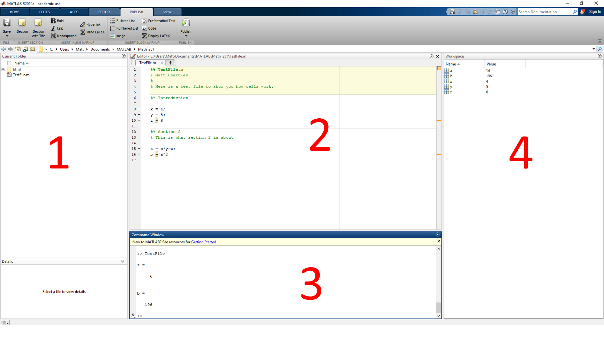
The MATLAB window has many parts to it. Here's how I like to set mine up.
The important components here are
You can set this up however you want, but I found that this works for me. You can drag the different windows around and resize the components.
You can run basic math operations in the command line window. This is the section beginning with the '>>' prompt. For instance, after that, you can type
2 + 3
press ENTER to evaluate the line and get the output
ans =
5
You can also then type
2*3*4;
press ENTER, and get no output. What happened? If you look in the variable window, you'll see that the variable ans still exists and has value 24. The semicolon at the end of the line suppresses output. The operation still goes through, but nothing shows up on the command line screen. The same works for scripts; including a semicolon at the end of the line will not show any output (which you should do while writing scripts), and when you intentionally remove the semicolon at the end of the line, the result of the calculation will show.
For script files, you can just write lines of code one after another. For instance, you can write something like
x = 15;
y = 2*3;
z = x-5;
a = x+y+z;
b = a^2
and then click the green "Play" button to run the script. At the end of this, you should see the output
b =
961
after you save the file.
Script files are saved as ".m" files, which you can reopen whenever you need in MATLAB. The command line data can not be saved so the only way to keep information to save is by writing it in a script file.
Comments in script files are written with % at the front of the line. In addition, you can add "Cells" to the file by starting a line with a %%. A practice that I like for files is to put one of these at the start of the file, %% with the title, and then comments under it with my name and data about the file. This make things look really nice when you go to publish files.
For this class, in particular, MATLAB Live Scripts will be used for the MATLAB assignments. These allow the MATLAB code to be viewed side-by-side with the output, as well as an easy export to PDF functionality. These are saved as '*.mlx' files. These work the same way as scripts in terms of how code is written, and allow the user to mix between text (which can be resized and formatted) and code. For more information on Live Scripts, see the website here. Live Scripts also have the ability to put section breaks between different pieces of code and then run individual sections using the ''Run Section" button at the top of the editor. With Live Scripts, it is necessary to run the entire code (by clicking the run button) before exporting as a PDF in order to get the correct images and outputs in the final PDF. To export, go to Save at the top of the screen, click the down arrow under it, and select ''Export to PDF'' after running the code to regenerate all of the images.
For help when using MATLAB, you can type
help 'command'
into the command window, replacing 'command' with whatever you want to learn more about. If you don't know where to start with commands, you can go to Google. Just put in what you want to do, and search for suggestions. It will likely take you to the MathWorks help site, where you can read more on what MATLAB can do.
Basic arithmetic calculations can be done as before: +, -, *, /, ^ work exactly as expected, and can be done in both the command line and scripts. Whenever you do any calculations MATLAB will automatically convert everything to decimals. If you want to deal with exact values and simplification, you need to use symbolic variables. For instance, something like
z = sqrt(sym(2))
where the sym() tells MATLAB to make it a symbolic variable, then z will behave exactly like the square root of two. For example,
z^2 - 2
will evaluate to zero, while
sqrt(2)^2 - 2
evaluates to something very small, in my case, 4.4409e-16.
As shown in the above example, functions are indicated with parentheses. That is, you write the name of the function and put the arguments after it in parentheses. The help window will also indicate this fact. Other important commands that will be helpful in doing basic arithmetic are:
When you want to evaluate a symbolic expression (that is, get a decimal approximation of it), use the command vpa(x). If you need more or less decimal digits in this approximation, you can set the number of digits with digits(d) and then run the vpa command.
To start doing algebra in MATLAB, we need to talk about the different types of functions and how they can be used in different ways. Symbolic functions will allow you to do a lot of the standard algebraic operations you are used to within the MATLAB interface. For instance, you can do things like
syms x;
f = x^2 + 4*x + 3;
g = f^2*(x-1);
h = f + 2*g;
Then you can run things like expand(g) or factor(h) to see what those commands do. These commands will also work for non-polynomial expressions.
If you need to evaluate a symbolic expression at a particular value, you use the command subs(f,x,a) to plug the value a in for x in the symbolic expression f. This does not change the expression f, so you will either need to store this new expression or evaluate it immediately to use it later. In order to evaluate, you use the vpa command as before.
MATLAB also has other types of functions, namely those that you write yourself. These can be done in the same script file, in a separate file, or inline as anonymous functions. The easiest to use are the anonymous functions, which take the form
fx = @(x) x.^2 + 4.*x + 3
Note the use of .^ for the power indicator. This is the notation for "element-wise" operation, which is used when plugging multiple values into a function, either by you or by another method you are trying to use. If you are only plugging in one value, it's not critical, but it is good practice. For these functions, you can not factor or expand or do algebra with them, but they are more effective at being evaluated than symbolic functions. You can also plot these functions as well, as shown in the graphing section. In general, you will want to stick with symbolic functions for this class, but there can be times when these functions are useful. If you want to convert a symbolic function to an anonymous function, you can do so with g = matlabFunction(f).
MATLAB will do integrals of anonymous functions via the integral(f, x_0, x_1) command. You can add options to change the quadrature rules, but that's pretty much all you can do with anonymous functions. If you want to go beyond that, you need to use symbolic functions, which you will see in this class, but will not need to code on your own.
Graphing in MATLAB can be done with lists of values, anonymous functions, or symbolic functions. For the first two, you will use the plot command on lists of values, which can be generated from the anonymous function as well. For example
xPts = [1,2,3,4,5];
fx = @(x) x.^2 + 2;
yPts = [2,3,2,3,1];
figure(1);
plot(xPts, yPts);
figure(2);
plot(xPts, fx(xPts));
This code should have generated two figures. The lines figure(1) and figure(2) refer to the two different figures, and allow you to make sure that the different graphs overlap. Whenever you draw a plot on a figure that already exists, it will overwrite that figure. If you need to put two plots on the same graph, you need to use the hold on; command as in the next example. You can use hold off; to undo this once you are done.
xPts = linspace(1,5,100);
fx = @(x) x.^2 + 2;
gx = @(x) x.^2 - 3*x + 7;
figure(1);
hold on;
plot(xPts, fx(xPts));
plot(xPts, gx(xPts));
hold off;
The linspace generates a list of 100 equally spaced values between 1 and 5 for plotting purposes. It allows you to get smoother plots than writing out a full list. There are also ways to plot multidimensional functions in this way, but they are trickier and not really necessary for this class.
For more information on all of these things, check out the MATLAB help documentation online. It is very helpful at learning how to do all of this.
If you want to print a simple variable during a script, you can do that by removing the semicolon from the end of the statement. On the other hand, if you are looking to just type text, you can do that inside of a comment. However, sometimes you want to print something more fancy, like a sentence that includes the value of a variable. To do that, you need another command, fprintf. This allows you to write words and put the value of variables inside of it. Here's an example.
a = 10;
b = 21;
fprintf('The variables are %s and %s.\n', num2str(a), num2str(b));
This should give you a good idea for how this command works. The important new commands here are:
There are many other options to use with the fprintf function, which you can find here.
For loops are a form of iterative programming, where you can have MATLAB run the same bit of code multiple times with an iterative parameter that can change certain things about the code. A sample for loop has the following form:
for counter = 1:1:10
CODE HERE
end
In this line, counter is the variable that is getting incremented over the list. The rest of that line says that counter starts at 1, increments by 1 each loop, and stops after 10. A line of the form counter = 2:5:34 will start at 2, increment by 5 each loop, and stop once the counter gets above 34, so after the loop at 32.
If statements, or conditional statements, allow certain parts of code to be executed only if a certain condition is met. For instance, something like
if counter < 5
CODE HERE
end
will only execute if the counter is less than 5, and
if mod(counter,2) == 0
CODE HERE
end
will only run if counter is even, that is, if the remainder when dividing counter by 2 is zero. Notice the == used for comparison here, where = is used for assignment.
One other thing you may want to do while writing these programs is loop through a list of possibilities and do some operation on each of the options. Thus, you have a list, you want to go through it one by one, and compute something for each of the options. You can do that with code like this.
v = [1,2,3,4,5]; % This will be your list of values
for counter = 1:1:length(v)
x = v(counter)^2
end
If the list you have is more complicated, you can use size to look at how big an array is to know what your loop parameter should go to. Look at the MATLAB help documentation to learn more about that.
There are several pre-written methods that are provided for these assignments that you will need to utilize to successfully complete them. Each of the methods contains some documentation at the top explaining how to properly use the method. To find this, you should open the file in MATLAB and read the part right under the function header. Here are some other notes that may help with using these files.
f = @(t,y) t^2 + y^2
and then can be passed into these functions just using the letter f. If you want to restrict a variable when you do this (like the single variable function f(1,y)), you could do so by passing@(y)f(1,y)
in place of the letter f.Documentation for all of the pre-written code can be found in the PDF here. All of the pre-written code needed is contained in the zip file here.
Euler's Method is the simplest and most direct way to numerically model a differential equation. The basic process is
The looping structure of this method makes it a great candidate for a for-loop (or a while loop). In addition, we want to structure this for-loop so that we track all of the $t$ and $y$ values that we obtained throughout the iteration (which makes the for-loop easier).
To write this method, the best practice would be to pre-allocate your memory for the $t$ and $y$ arrays, which you can do by using the $dt$ parameter and the initial and final times to see how many steps you'll need to complete the process. Once building these vectors, you'll want to step through Euler's method one step at a time, compute the next $t$ and $y$ values in each iteration of the loop, making sure to store the new values at the proper index. Once the loop finishes, this should give you the full array of values that you want out of this method.
MATLAB has several built in methods that numerically solve ODEs, and these are generally more complex than the simple Euler's method described above. The most commonly used of these is ode45. The best way to learn about these methods is via the MATLAB documentation. I have always found it helpful for at least getting started and being able to use a method. Google will get you there pretty quickly, but the documentation for ode45 is here: https://www.mathworks.com/help/matlab/ref/ode45.html.
The important things to learn from this is how to input things to the function. For example, the documentation here tells us that the proper input for this function is
[t,y] = ode45(odefun, tspan, y0)
where odefun is an anonymous function of two variables in the order t, y, and we want to solve the equation or system $y' = f(t,y)$. The tspan is a two-element array with the starting and ending $t$-values, and y0 is the initial value at t0.
If you aren't sure how to use any of this, the MATLAB documentation also has several examples of the code written out in detail for this process. Those can give you ideas for how to structure your code to get it to work.
All of MATLABs built-in methods have this kind of documentation, so you can look up how they work as well as code snippets of how to use them. In terms of using MATLAB, this is one of the best features. It won't solve all your problems, but it will likely get you headed in the right direction.
When drawing multiple graphs at the same time, it can be helpful to specify different properties of the curve to tell them apart. The full details of what can be done here is in the MATLAB Documentation here. The basic details are that you can pick the line-style (solid, dashed, dotted), color, and marker type of each curve separately. For instance, using 'ob' as the LineSpec will give blue open circles at each value that you input. Using '--r' will give a red dashed line, but no individual markers at each point. Skim through that documentation page to figure out how you want your plots to appear.
In addition, including legends and axis labels can be very helpful in making your figures clear and understandable. The information about legends can be found here and more generic information about graph annotations can be found here..
There may be some cases where your code is not running as fast as you would like, or you want to rapidly test the code without needing to wait for a full size data set to run. In this case, you can cut down some of the factors to make it run faster and get a better picture of what's going on. In terms of the function you will be writing, you can reduce the number of points at which you start the fsolve calculation. This may cause you to miss some zeros, but it will run faster. In addition, you could reduce the number of red or blue lines that you draw for the picture process; that will also speed up the calculations.
The pre-written method bifdiag244.m can be notorious for this. There are basically nested loops in here, and too many of any one parameter value can easily make things spiral out of control. If you are having difficulty with this method and it is taking too long to run, there are two parameters you can change. The first is the NLines variable at the top. The higher this number is, the more lines are drawn, and the longer the code will take. A large value here makes for great pictures, but it can take forever to draw. You can drop this slightly if it is taking too long. The other value is the 25 in line 22. This could also be made smaller if needed, but the NLines part is really the determining factor of speed here.
You will need to utilize more prewritten code for this assignment, and the methods are fairly short when written out, and can be hard to understand. For the drag coefficient methods, the first method is:
function [t,v] = dragSolution(gamma, Tf)
f = @(t,v) 9.8 - gamma.*v.^2;
[t,v] = ode45(f, [0, Tf], 0);
end
This method has two inputs, a value for the parameter gamma and a final time Tf. The first line sets up the function that defines the differential equation for the velocity. Then, the second line numerically solves the differential equation $v' = f(t,v)$ and returns the values of t and v that were computed here. To run this method, you pass in a value for gamma and an end time Tf, and then this method will compute the solution for you.
The next method dragSolutionVals does the same thing, but computes the solution at a specified set of tVals. The last method does the optimization process:
function optGam = dragOptimization(tVals, vVals)
testVals = @(gamma) dragSolutionVals(gamma, tVals);
testError = @(gamma) sum((testVals(gamma) - vVals).^2);
optGam = fminbnd(@(a) testError(a), 0, 1);
end
The inputs to this function are the given data in the form of a vector of t values and a vector of v values. The first line of the code defines a function of gamma that gives the solution to the differential equation with that gamma, at the provided list of t values. The second line defines another function of gamma giving the error between these test values and the given v values. Finally, the last line uses fminbnd from the Optimization Toolbox to compute the value where this error function is minimized, returning that value. Thus, the code looks to find the best possible choice for gamma that will best fit the data for this function, so is our best guess to what this gamma is from the data.
The three methods for the harvesting function work the same way. It uses fmincon instead of fminbnd because we need to optimize over three variables instead of just 1. The idea of all of this is the same.
For a few components of this assignment, code using the MATLAB Symbolic Toolbox is provided to you. (Note: If you do not have the toolbox installed, you may need to do so in order to run this code). For the first instance of this, you will not need to edit this code at all. It is there to show you that MATLAB can generate the appropriate solution to this differential equation symbolically.
For the last problem in the lab, you will need to utilize the code a little bit to solve the second differential equation given in the problem. To do this, you should read through the code to see what it does (the symbolic code is usually pretty obvious in what it is doing) and then copy the code a second time, changing the necessary components to make it solve the second differential equation. You'll want to call all of the new variables y2(t), Dy2, ySol2 in parallel with the original solution. This will allow you to do the same thing, but for the new set of coefficients, keeping the two solutions second. You will also need to rewrite the conds vector, as this also needs to refer to the y2 solutions.
If you do it this way, the plotting commands are already at the bottom of this section and will show what these solutions look like. If there are issues, the documentation on the fplot function may be helpful.
MATLAB has a interesting feature that allows it to play sound from the graph of a function. Two built-in examples within MATLAB are available in handel.mat and gong.mat. These can be run by evaluating the following commands in the Command Window:
load handel.mat
sound(y, Fs)
Be careful with your computer volume when running these commands, as it may be loud. For something a little more recognizable (at least for those with a slight exposure to music theory) the function
tVals = linspace(0, 2, 2*8192);
A = @(x) sin(2*pi*220*x);
sound(A(tVals));
will generate a single pitch equivalent to the A below middle C on a piano. For more fun work with this, check out this MATLAB file.
This is what you will be using to ''visualize'' the results from the calculations of Question 6 on the lab. You can look at what is happening just from the graph, but it can be easier to get a feel for the phenomenon involved by hearing it. Once you generate an oscillatory function, which you can get from the secondUndampedSolver function, you will need to generate a MATLAB anonymous function from it. This can be done by taking the outputs from your function and writing
soln = @(t) Ac.*cos(omegas*t) ...
continuing to include the rest of the terms. Once this is together, the line sound(soln(tVals)) will play the ''sound'' that is given by that solution. Experiment with this to see what the different solutions sound like, and then you can comment this out of the file before you go to publish it.
MATLAB is built to handle matrices, and so the methods to work with them are pretty straight-forward. Vectors in MATLAB are handled by arrays, which are lists of values that MATLAB stores in a single variable. In most cases, they can be done with either horizontal arrays
v = [1,2,3];
or vertical arrays
w = [1;2;3];
where comma indicate breaks in a horizontal array and semicolon gives the breaks in a vertical array. In particular, semicolons always indicate breaks between rows in a vector, which is the same for a matrix. If we want to store a 2x2 matrix, we can do so by
M = [1, 2; 3, 4];
which will give the matrix $\displaystyle M = \left( \begin{matrix} 1 & 2 \\ 3 & 4 \end{matrix}\right)$. In order to access the elements of a matrix, they are accessed using parentheses, just like vectors. For a vector v(2) will access the second element of a vector $v$, and for matrices, M(1,2) will access the element of $M$ in row 1, column 2. Therefore, for the matrix $M$ above, M(2,1) will return 3. If you try to ask for M(1,3) MATLAB will give you an Index out of Bounds error, because you are trying to access the third column of the matrix, which doesn't exist.
A colon can be used to access an entire row of a matrix at once. For instance, if we have the matrix
M = [1,2,3;2,3,4;4,5,6];
as a 3x3 matrix, the command M(1,:) will return the vector [1,2,3], as it will give the first row of the matrix. The same goes for M(:,2) giving back [2;3;5].
A lot of MATLAB's methods can handle matrices as inputs. If you are curious about an individual method, the MATLAB documentation on the method should detail what exactly can be a matrix and what can not.
The goal of this lab is to introduce the idea of phase portraits. Phase portraits are used for first order autonomous systems to get an idea of how the system behaves when it can be difficult to predict just based on small amounts of information. They are a generalization of phase lines to a two component system.
To draw phase portraits, the main point is that we want to plot x vs. y instead of plotting x and y vs. t. This can be done fairly easily in MATLAB. If we have a solution of the form $x(t)$ and $y(t)$, we could take a collection of t values $tV$ and plot the solutions $x(t)$ and $y(t)$ using
plot(tV, x(tV));
plot(tV, y(tV));
However, if we want to plot x vs. y, we can do that just as easily with
plot(x(tV), y(tV));
since this will plot the x-component in the horizontal direction and the y-component in the vertical direction. Doing this for a bunch of different initial conditions will draw a full phase portrait.
There are several convenient ways to generate vectors with a large number of elements at once, provided they satsify a nice pattern. To get a vector with the same value many times, this can be done with using the function ones(1, n) , which generates a vector with n entries, all of which are 1. It can then be multiplied by a number to get whatever vector is needed. The other option is to use the colon operator. For example,
1:5
will generate the vector [1, 2, 3, 4, 5] . That is, it automatically uses a spacing of 1. If a spacing other than 1 is desired, it can be done with something like
1:0.1:5
which will generate a vector of [1, 1.1, 1.2, ..., 5], which is from 1 to 5, with 0.1 between each entry.
For most of the necessary background information, look at the lab assignment document. Most of the problems for this lab will involve playing with different parameters and seeing how it affects the overall results.
The example code in the format file shows how subfigures work, which is a neat way in MATLAB to show mutliple plots side-by-side. The basic code in MATLAB is
figure();
subplot(2, 1, 1);
plot(...);
subplot(2, 1, 2);
plot(...);
The subplot(m, n, k) sets up a figure with m rows, n columns, and puts this figure in the kth spot of that array. The example above makes an array of 2 rows, 1 column, and then puts the appropriate plots in the right order. There is a lot more that can be done with this to generate some interesting plots; more information can be found here.