MATLAB is a computer system that focuses more on the numerical side of calculations as opposed to symbolic calcuations. It has the capability to do symbolic calculations, but the base software is more inclined towards numerical computations. It is one of the industry standard computational programs in engineering, and is fairly commonly used outside of academia.
MATLAB can be run both through a command-line type prompt and scripts, lines of code that will be executed in sequence. In general, the command line prompt is used for testing code, accessing help functions, and making sure MATLAB works as intended, and scripts are used for putting together programs that solve problem sets or carry out certain tasks. For the computational labs, you will be expected to write scripts containing your solutions. If it is your first time trying to do a certain type of problem, it would be useful to run the code line by line (in the script file) and then testing what you want to write next in the command line before you add it to the script.
MATLAB can also generate pictures and graphs of functions, and has a straightforward way to modify colors and sizes and put legends on the axes. These are mostly done from a coding-type interfaces, so they are a little trickier to show and view correctly, but the numerical capabilities make up for it. Within scripts, one can also write functions where one can write sequences of commands (with inputs and outputs) that can be saved and executed repeatedly within a single script. They can also be imported to other script files to carry these methods over to them.
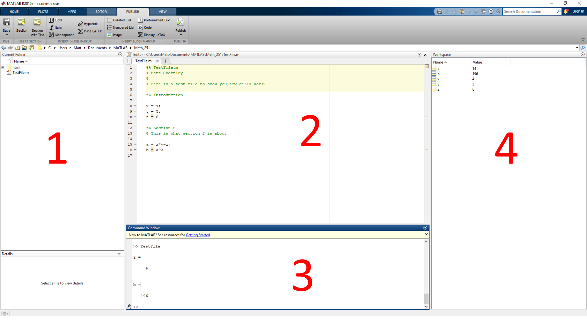
The MATLAB window has many parts to it. Here's how I like to set mine up.
The important components here are
You can set this up however you want, but I found that this works for me. You can drag the different windows around and resize the components.
You can run basic math operations in the command line window. This is the section beginning with the '>>' prompt. For instance, after that, you can type
2 + 3
press ENTER to evaluate the line and get the output
ans =
5
You can also then type
2*3*4;
press ENTER, and get no output. What happened? If you look in the variable window, you'll see that the variable ans still exists and has value 24. The semicolon at the end of the line suppresses output. The operation still goes through, but nothing shows up on the command line screen. The same works for scripts; including a semicolon at the end of the line will not show any output (which you should do while writing scripts), and when you intentionally remove the semicolon at the end of the line, the result of the calculation will show.
For script files, you can just write lines of code one after another. For instance, you can write something like
x = 15;
y = 2*3;
z = x-5;
a = x+y+z;
b = a^2
and then click the green "Play" button to run the script. At the end of this, you should see the output
b =
961
after you save the file.
Script files are saved as ".m" files, which you can reopen whenever you need in MATLAB. The command line data can not be saved so the only way to keep information to save is by writing it in a script file.
Comments in script files are written with % at the front of the line. In addition, you can add "Cells" to the file by starting a line with a %%. A practice that I like for files is to put one of these at the start of the file, %% with the title, and then comments under it with my name and data about the file. This make things look really nice when you go to publish files.
Once you are done with the script file and are ready to submit the assignment, you can generate a file for submission using the Publish function (under the Publish tab at the top of the page). If you click that button, it will run your entire file and format the result into an HTML file. It will use the different "Cells" as sections in the file, and will make your document look nicer.


For help when using MATLAB, you can type
help 'command'
into the command window, replacing 'command' with whatever you want to learn more about. If you don't know where to start with commands, you can go to Google. Just put in what you want to do, and search for suggestions. It will likely take you to the MathWorks help site, where you can read more on what MATLAB can do.
Basic arithmetic calculations can be done as before: +, -, *, /, ^ work exactly as expected, and can be done in both the command line and scripts. Whenever you do any calculations MATLAB will automatically convert everything to decimals. If you want to deal with exact values and simplification, you need to use symbolic variables. For instance, something like
z = sqrt(sym(2))
where the sym() tells MATLAB to make it a symbolic variable, then z will behave exactly like the square root of two. For example,
z^2 - 2
will evaluate to zero, while
sqrt(2)^2 - 2
evaluates to something very small, in my case, 4.4409e-16.
As shown in the above example, functions are indicated with parentheses. That is, you write the name of the function and put the arguments after it in parentheses. The help window will also indicate this fact. Other important commands that will be helpful in doing basic arithmetic are:
When you want to evaluate a symbolic expression (that is, get a decimal approximation of it), use the command vpa(x). If you need more or less decimal digits in this approximation, you can set the number of digits with digits(d) and then run the vpa command.
To start doing algebra in MATLAB, we need to talk about the different types of functions and how they can be used in different ways. Symbolic functions will allow you to do a lot of the standard algebraic operations you are used to within the MATLAB interface. For instance, you can do things like
syms x;
f = x^2 + 4*x + 3;
g = f^2*(x-1);
h = f + 2*g;
Then you can run things like expand(g) or factor(h) to see what those commands do. These commands will also work for non-polynomial expressions.
If you need to evaluate a symbolic expression at a particular value, you use the command subs(f,x,a) to plug the value a in for x in the symbolic expression f. This does not change the expression f, so you will either need to store this new expression or evaluate it immediately to use it later. In order to evaluate, you use the vpa command as before.
MATLAB also has other types of functions, namely those that you write yourself. These can be done in the same script file, in a separate file, or inline as anonymous functions. The easiest to use are the anonymous functions, which take the form
fx = @(x) x.^2 + 4.*x + 3
Note the use of .^ for the power indicator. This is the notation for "element-wise" operation, which is used when plugging multiple values into a function, either by you or by another method you are trying to use. If you are only plugging in one value, it's not critical, but it is good practice. For these functions, you can not factor or expand or do algebra with them, but they are more effective at being evaluated than symbolic functions. You can also plot these functions as well, as shown in the graphing section. In general, you will want to stick with symbolic functions for this class, but there can be times when these functions are useful. If you want to convert a symbolic function to an anonymous function, you can do so with g = matlabFunction(f).
MATLAB will do integrals of anonymous functions via the integral(f, x_0, x_1) command. You can add options to change the quadrature rules, but that's pretty much all you can do with anonymous functions. If you want to go beyond that, you need to use symbolic functions.
For symbolic functions, MATLAB can compute limits, derivatives, and integrals. For instance,
syms x
f = exp(4*x) + x^2 + 3*x + 1
g = x / abs(x)
limit(f, x, 2)
limit(g, x, 0, 'left')
limit(g, x, 0, 'right')
limit(g, x, 0)
Run these commands. Hint: Think about what the function g looks like and why this makes sense. Also
diff(f, x)
diff(f, x, 2)
int(f, x)
int(f, x, 1, 6)
You should run these as well to see how they work. They are pretty straight-forward. If you need to do numerical integration, you can either run vpa outside of int, or use the command vpaintegral in the same way you would use int.
Graphing in MATLAB can be done with lists of values, anonymous functions, or symbolic functions. For the first two, you will use the plot command on lists of values, which can be generated from the anonymous function as well. For example
xPts = [1,2,3,4,5];
fx = @(x) x.^2 + 2;
yPts = [2,3,2,3,1];
figure(1);
plot(xPts, yPts);
figure(2);
plot(xPts, fx(xPts));
This code should have generated two figures. The lines figure(1) and figure(2) refer to the two different figures, and allow you to make sure that the different graphs overlap. Whenever you draw a plot on a figure that already exists, it will overwrite that figure. If you need to put two plots on the same graph, you need to use the hold on; command as in the next example. You can use hold off; to undo this once you are done.
xPts = linspace(1,5,100);
fx = @(x) x.^2 + 2;
gx = @(x) x.^2 - 3*x + 7;
figure(1);
hold on;
plot(xPts, fx(xPts));
plot(xPts, gx(xPts));
hold off;
The linspace generates a list of 100 equally spaced values between 1 and 5 for plotting purposes. It allows you to get smoother plots than writing out a full list. There are also ways to plot multidimensional functions in this way, but they are trickier and not really necessary for this class.
Plotting symbolic functions is easier than for anonymous functions. The command fplot will plot both single variable functions and two-variable parametric equations.
syms x t;
f = x.^2 + 3*x + 1;
r1 = cos(2*t);
r2 = sin(3*t);
figure(1);
fplot(f, [-3,3]);
figure(2);
fplot(r1,r2, [-2*pi, 2*pi]);
You can also use the hold on commands with these plots as well. The other commands like this are fimplicit for plotting implicit functions of two variables, fimplicit3 for an implicit function of 3 variables, and fsurf for a surface of the form z = f(x,y). For more information on how to use these functions, the help page can be found here.
For more information on all of these things, check out the MATLAB help documentation online. It is very helpful at learning how to do all of this.
If you want to print a simple variable during a script, you can do that by removing the semicolon from the end of the statement. On the other hand, if you are looking to just type text, you can do that inside of a comment. However, sometimes you want to print something more fancy, like a sentence that includes the value of a variable. To do that, you need another command, fprintf. This allows you to write words and put the value of variables inside of it. Here's an example.
a = 10;
b = 21;
fprintf('The variables are %s and %s.\n', num2str(a), num2str(b));
This should give you a good idea for how this command works. The important new commands here are:
There are many other options to use with the fprintf function, which you can find here.
For loops are a form of iterative programming, where you can have MATLAB run the same bit of code multiple times with an iterative parameter that can change certain things about the code. A sample for loop has the following form:
for counter = 1:1:10
CODE HERE
end
In this line, counter is the variable that is getting incremented over the list. The rest of that line says that counter starts at 1, increments by 1 each loop, and stops after 10. A line of the form counter = 2:5:34 will start at 2, increment by 5 each loop, and stop once the counter gets above 34, so after the loop at 32.
If statements, or conditional statements, allow certain parts of code to be executed only if a certain condition is met. For instance, something like
if counter < 5
CODE HERE
end
will only execute if the counter is less than 5, and
if mod(counter,2) == 0
CODE HERE
end
will only run if counter is even, that is, if the remainder when dividing counter by 2 is zero. Notice the == used for comparison here, where = is used for assignment.
One other thing you may want to do while writing these programs is loop through a list of possibilities and do some operation on each of the options. Thus, you have a list, you want to go through it one by one, and compute something for each of the options. You can do that with code like this.
v = [1,2,3,4,5]; % This will be your list of values
for counter = 1:1:length(v)
x = v(counter)^2
end
If the list you have is more complicated, you can use size to look at how big an array is to know what your loop parameter should go to. Look at the MATLAB help documentation to learn more about that.
Vectors in MATLAB are represented by arrays, which are also called vectors in MATLAB. MATLAB automatically does addition and subtraction of vectors element-wise, in exactly the way you would want them to. That is, the code snippet
p = [1,2,3];
q = [4,6,8];
p + 2*q
will return the output 9 14 19 as expected. You can do element-wise multiplication of vectors with .* , which is not something done directly in Calculus 3, but it could be useful for doing dot products when combined with the sum function. In this case, the product p.*q is 4 12 24.
One other important thing to know about MATLAB is that everything is a matrix, so there are two types of vectors, row vectors and column vectors. Row vectors have commas between each element, and column vectors has semi-colons. There are a few cases where you want to use column vectors vs. row vectors, but most of the time it doesn't matter. However, you can't add column vectors and row vectors to each other. However, if you multiply a column vector by a row vector (in that order), it will do the matrix product, which is equivalent to the dot product. The other way around gives you something very different. For example, you can run this code to see what happens.
p = [1,2,3];
q = [4;6;8];
q*p
p*q
If you want to change a row vector into a column vector, you can do that with the transpose function or putting an apostrophe (') after the vector. This will rotate the vector, giving you a column vector if you put in a row vector, and vice versa. Note: The apostrophe actually does Hermitian transpose, which also conjugates complex numbers in addition to rotating the vector. That shouldn't matter for this class, but for future reference.
To access individual elements of a vector, you use parentheses. From the code above, q(2) will give you the number 6. For instance, if you wanted to compute the cross products of two vectors, the first component would look something like v(2)*w(3) - v(3)*w(2). You can figure out the rest.
MATLAB has built in trigonometric functions. Sin, Cos, and Tan are fairly straight-forward. For the inverse functions, asin acos are what you are looking for. Use help asin and help acos to figure out how to use them. Be careful about the range of these functions (which is given in the help screen).
For part of this lab, you will need to draw polygons and lines. For this, we will take advantage of the fact that if we tell MATLAB to plot two points, it will draw the line between them. In addition, if we tell MATLAB 3 points, it will draw two line segments, from A to B, and from B to C. To make this work conveniently, we'll want to use the matrix capabilities of MATLAB.
Here's an example of what we want to do. Say we have two row vectors
p = [1,2,3];
q = [4,6,8];
and I want to draw the line from p to q. Using these vectors, we can define the matrix M by
M = [p;q];
which is going to stack p and q on top of each other in the matrix M. Now, matrices have two indices, the first for the row, and the second for the column, and putting in : for either of these entries will grab all of them. Thus if I do M(1,:), this will grab the first row of the matrix M, which is p, and M(2,:) will grab q. The important part of this that I want to look at is M(:,1) which will grab the first column of M, which is both of the x coordinates of these vectors.
That leads in well to how we plot things in MATLAB. The three dimensional plot command is
plot3(xCoords, yCoords, zCoords)
where xCoords, yCoords, and zCoords are vectors of the same size (same length) representing the x, y, and z coordinates of the points that you want to plot. For example, to plot the line between p and q from before, we could use the code
plot3(M(:,1), M(:,2), M(:,3));
You can replace p and q with whatever points you want in order to draw lines. For instance, if you wanted to draw the line starting at v in the direction of n, you could replace p by v and q by v+n.
For drawing filled in polygons, you can do the same sort of thing. The command you want here is fill3 instead of plot3, but the rest is the same. fill3 also requires a fourth argument, which is the color of the fill. More detail can be found about this here.
Finally, we want to be able to generate good pictures with script files instead of just when we modify figures by hand. The way you can do this is by setting a view argument after generating the figure. When you make a MATLAB figure, either with a script or via the command line prompt, you can rotate it. Click on the image, and then click on the rotation icon circled below.

Once you click on this, then you can click and drag around the image to rotate it to get a better view. You'll want to make sure that you can see everything clearly as well as how things interact. However, if you re-run the code, you'll get back to the same picture you started with. To get the image you actually want in the code, you can include a view command to set the angle appropriately. Once you rotate an image to get the picture you want, you can get the view argument by opening the Property Inspector, scrolling down to viewing angle, and looking the view parameter.

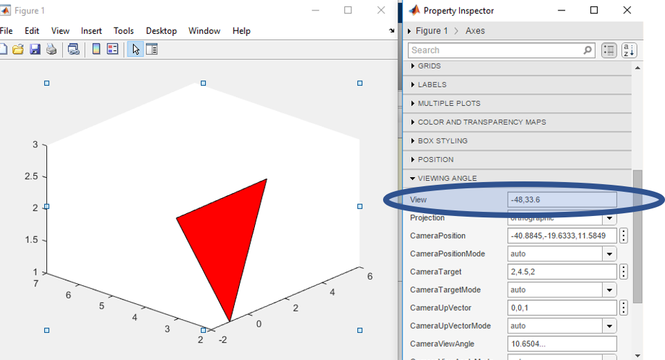
Finally, you can, after generating the image, type the command view(a,b), where a,b are the numbers in the view argument. Then, when you run the code, the image that appears will be the one that you want. If there are other properties you want to change, you can also find them in the Property Inspector and put commands into the script to modify the picture.
In order to print the equations of the plane, you'll want to use fancier print statements. Those can be done in this form. Here's an example.
a = 10;
b = 21;
fprintf('The variables are %s and %s.\n', num2str(a), num2str(b));
This should give you a good idea for how this command works. The important new commands here are:
You can modify this in order to put the equations where you need them in the file, and use components of the normal vector within the statement.
For these instructions, we will be using as an example the curve given by:
r(t) = < 5 cos(2t) + 5 sin(t), 2 cos(2t) + 4 cos(t), sin(3t) + 4 sin(t)>
or if you prefer the parametric notation:
x=5 cos(2t) + 5 sin(t)
y=2 cos(2t) + 4 cos(t)
z= sin(3t) + 4 sin(t)
I'm beginning with this curve because it is fairly simple. More complicated curves will appear later. This curve is a closed curve (i.e. a loop) on the interval [0,2π] because the formulas are all combinations of sines and cosines with integers multiplying the parameter, t.
In order to plot this correctly, we need to use the parametric formulation. Unfortunately, Matlab doesn't know how to handle vector valued functions, so it has to be done manually. We can store this function by
syms t;
x(t) = 5*cos(2*t) + 5*sin(t);
y(t) = 2*cos(2*t) + 4*cos(t);
z(t) = sin(3*t) + 4*sin(t);
and then we can draw the curve by
fplot3(x(t), y(t), z(t), [0, 2*pi]);
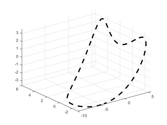
which produces the following picture.

This picture is pretty good. If we want more control over the picture, we can change some options on it. The options are separated by commas after the t-range you specify.
For example, if we use the command
fplot3(x(t), y(t), z(t), [0, 2*pi], '--k', 'LineWidth', 3);
Then we get the picture
Consider the following picture of the curve, s(t)=< sin(2t), cos(2t), sin(t) >
This shares the a figure-8 shape with our original picture of our curve r(t). This curve actually has an intersection, however, as illustrated by the animation below. We'll discuss how to make these kinds of animations later.
Since you cannot print an animation, you should include several views of your curve to convince the reader of any intersections.
Warning: There are curves which do not intersect themselves, but have the irritating (interesting?) property that every two dimensional view shows intersections! See the bottom of this page for examples. For example, q(t)=<sin(t),cos(3t),sin(2t)> (animated below) has this property. In this case you would include several views of your curve to convince the reader that there are no intersections.
Watch as intersections appear and disappear. Compare this to a curve with an actual intersection, such as s(t)=<sin(2t), cos(2t), sin(t)> above where the intersection does not disappear. More examples of such curious curves appear at the bottom of this page.
Unfortunately, drawing animations in Matlab is not as simple as it is in the other algebra systems. We can still do it, but it requires a little more heavy lifting on the code part. Essentially, we need to write the loop that will draw all of the different figures.
Let's say we want to animate a point moving around the r(t) curve in 100 frames from t=0 to t=4*pi. This means it will circle the curve twice. To do this, we first need to pick out the time values for each of the frames.
pts = linspace(0, 4*pi, 100);
Next, we need to draw the plot. This is going to consist of both the entire curve and the individual point that is moving around it. We need to do this inside of a for loop in order to get each plot separately.
for k=1:length(pts)
fplot3(x(t), y(t), z(t), [0,2*pi], '-k', 'LineWidth', 2);
hold on;
plot3(x(pts(k)), y(pts(k)), z(pts(k)),'r.', 'MarkerSize', 30);
hold off;
M(k) = getframe;
end
The fplot3 command draws the curve, like we saw before, and the plot3 command draws the individual point that is tracking around it. We need to, at each step, move forward one more t value (by imcrementing k) to get through the entire curve. The hold on; and hold off; commands allow the two plots to be drawn on the same axes, but then clear the point away before we draw a new one. The M(k) = getframe;<\span> stacks all of the images together so that the command
movie(M)
will play the movie. For this set of commands, we get the following animation.

Note: It is actually a lot harder than this to save animations in Matlab. I had to jump through a few more hoops to get a gif saved that I could put on this website. Thankfully, you just have to look at the animation to see what's going on, so the movie command will work just fine for you.
How long is this curve? This is called the arc length, which is calculated by integrating the speed of r(t) for the desired range of t (i.e. ∫ab |r'(t)| dt ). We need to differentiate r(t), and then find its length or magnitude (this is the speed). Since we already have r(t) in component form, we can use that to compute the speed.
speed(t) = sqrt(diff(x(t),t)^2 + diff(y(t),t)^2 + diff(z(t),t)^2);
Note: For the type of functions that you will have in this assignment, Matlab was being annoying in simplifying the functions appropriately to be able to integrate them. To fix this, you can use the command:
speedsim(t) = prod(sqrt(factor(simplify(expand(speed(t)^2)))));
which, if you read it, squares the speed, expands out everything, simplifies it, factors into different terms, takes the square root of each of these factors, and then multiplies them together. This does not change the expression at all (in terms of a mathematical sense) but does allow Matlab to interpret it properly. Wherever you see speed in the code snippets below, you should replace them by speedsim so that Matlab handles things properly.
We are interested in the length of one loop of the curve. For our curve "one loop" is given by the range 0 ≤ t ≤ 2π, so we need to integrate speed from t=0 to t=2*Pi to get the length. We can integrate using the int command, so may naturally try:
int(speed(t), t, 0, 2*pi)
which will cause Matlab to just return the formula. To get the actual value, you can type double(ans);, or just put double in front of the int command. Note: If you want to use this length later in the assignment (hint hint), you should save the version with double as a variable, that way it can do things later. Doing that gives
56.131895615918667430156501433069
as the length of the curve.
The other main part of this lab is computing an arc length parametrization for the curve. The background file for this lab gives a step-by-step process for doing this.
syms tau;
L(t) = int(speed(tau), tau, 0, t);
syms s;
solve(s == L(t), t);
Note the use of the == to set up equality here; Matlab needs that to know how to handle the solve command. You'll then want to save the function that comes out as g(s). However, I was having issues with making this work properly. The method that does work is using the finverse command, i.e.,
assume(t, 'positive');
g(s) = subs(finverse(L(t)), t, s);
At this point, we can then find r2 in terms of its parametric functions by settingx2(s) = x(g(s))
y2(s) = y(g(s))
z2(s) = z(g(s))
which, without the semi-colons, will display the functions. Aren't you glad you didn't have to do this by hand?
Some strange things can happen. Let me show you a few of them.
Below are three pictures of another curve. I emphasize that these are all pictures of the same curve. This curve does not intersect itself, but every two dimensional view does seem to show an intersection. So detecting intersections by "just looking" may be a bit difficult. Some examination of the images is necessary.
Here are two pictures of yet another closed curve. This closed curve does have two self-intersections, each of which can appear to be an illusion. It can be difficult to convince people of these intersections without much numerical work (e.g. showing that r(t0)=r(t1) for some 0 ≤ t0 < t1 < 2 π) or many carefully chosen pictures. If you have suggestions, please let me know.
What possible two-dimensional pictures can result from such an equation? Here are some examples.
This might be the most disturbing "picture". The equation x2+y2+1=0 is not satisfied by any pairs of numbers, (x,y), since the right-hand side is always positive. (Maybe this is an advertisement for complex numbers?)
Look at 29x2+2xy+10y2+8x+12y+4=0. Then realize this is the same as (5x-y)2+(2x+3y+2)2=0 because (5x-y)2=25x2-10xy+y2 and (2x+3y+2)2=4x2+9y2+4+12xy+8x+12y. I did this in reverse, actually, and started with the squares. But the only way that (5x-y)2+(2x+3y+2)2 can be 0 is if (squares are never negative!) 5x-y=0 and 2x+3y+2=0. The first equation gives y=5x and when substituted in the second equation you get 2x+3(5x)+2=0 so that x=-2/17 and then y=-10/17. So "clearly" (not so clearly to me!) the point (-2/17,-10,17) is the only solution to 29x2+2xy+10y2+8x+12y+4=0.
Just x+y=0 will do.
|
Certainly students should recognize x2+2y2-1=0 as an ellipse. But you may find it difficult to believe that 11x2-32xy+24y2+24x-40y+21=0 is also an ellipse. You could try the command fimplicit(11*x^2-32*x*y+24*y^2+24*x-40*y+21==0, [1,6,2,5], 'MeshDensity', 200); and see the result. You can also apply any of the normal options here that you would to normal plots. The new one here is MeshDensity, which determines how many points Matlab tries to evaluate in order to plot the curve. The default here is 151, which is large enough for pretty much anything you could want to do. (Maple's is smaller than that) For comparison, here are two plots with MeshDensity 25 and MeshDensity 151. |
With MeshDensity=25 |
|---|---|

| |
| No specification, so MeshDensity=151 | |

|
|
One simple example is x2+y=0. And, again, it may not be obvious that 25x2-40xy+16y2+13x-9y+3=0 is also a parabola, but displayed to the right is the result of this Maple command: fimplicit(25*x^2 - 40*x*y + 16*y^2 + 13*x - 9*y + 3 == 0, [-10,0,-10,0]); |

|
|
The model hyperbolas you have been told about include xy=1 and x2-y2=1. But -7x2-6xy+16y2+48x-80y+74=0 is also the equation of a hyperbola whose graph is shown to the right. |
|
Well, xy=0 is sort of a hyperbola. It is (sigh!) a degenerate hyperbola or limiting form of a hyperbola. For example, xy=0 is a pair of lines which intersect in one point, and this "curve" is certainly the limit of the curves xy=tiny number as tiny number-->0. Also two parallel lines can be described by a quadratic polynomial: the points (x,y) which satisfy x2=1 are the straight lines x=1 and x=-1. This is another "degenerate" case.
All of these curves are called conic sections.
We need to build a right circular cone. This is a cone with a central axis perpendicular to a plane.
Step 1Take a straight line (which will be the axis of symmetry of the cone), and take a plane perpendicular to the line. In the plane, imagine a circle whose center is the point of intersection of the line and the plane. Now fix a point on the line outside of the plane. |
|
Step 2Now draw a straight line through the external point and every point on the circle. This collection of lines will form a surface. Each of the lines is called a generator of the cone. The original line is the axis of symmetry of the cone. The external point is called the vertex of the cone. |
|
| The right circular cone looks like what is sketched to the right. Suppose this cone is sliced by another plane. A conic section is the resulting curve: the intersection of the cone and the plane. The type of the curve is determined by the angle made by the intersecting plane and the axis, and how this angle relates to the vertex angle of the cone. |
|
EllipseIf the angle made by the intersecting plane and the axis is greater than the vertex angle, then the plane will only slice through one of the cone's pieces. The resulting curve is an ellipse. |
|
HyperbolaIf the angle made by the intersecting plane and the axis is less than the vertex angle (or is parallel to the axis of symmetry), then the plane will slice through both parts of the cone's pieces. The resulting curve is a hyperbola. |
|
ParabolaIf the intersecting plane is exactly parallel to one of the generating lines (and that's darn unlikely for a random plane!) then the plane will slice through only one part of the cone. The resulting curve is a parabola. |
|
These geometric characterizations of the conic sections are thousands of years old. There are also definitions of the various conic sections using distance in the plane. For example, an ellipse is the collection of points the sum of whose distances to two fixed points is a constant.
If the universe were empty except for the sun (a heavy point mass) and an asteriod (a much lighter mass) than the orbit the asteroid would have around the sun would be a conic section. The textbook discusses this in the section on Kepler's laws. So these curves (motion in an inverse square law force field) will be everywhere in physics.
Suppose we want to know which conic section is given by Ax2+Bxy+Cy2+Dx+Ey+F=0. I'll assume that |A|+|B|+|C|>0, so that at least one of the quadratic coefficients is not 0. Otherwise we've just got a line or a point. The type of the curve depends on the discriminant. The discriminant is defined to be B2-4AC.
We looked at the ellipse 11x2-32xy+24y2+24x-40y+21=0 earlier, with A=11, B=-32, and C=24. The (-32)2-4(11)(24) turns out to be -32.
An example of a hyperbola earlier was -7x2-6xy+16y2+48x-80y+74=0. Here A=-7, B=-6, and C=16, so B2-4AC=(-6)2-4(-7)(16)=484>0.
I had claimed earlier that 25x2-40xy+16y2+13x-9y+3=0 was a parabola. Here (-40)2-4(25)(16)=0.
These algebraic statements are several hundred years also, and can be verified using high school algebra, but the "high school algebra" must be applied very diligently. Some students might see a resemblance in the discriminant analysis and consequences to the second derivative test for functions of two variables, and the resemblance is not accidental. The second derivative test actually uses these results in a somewhat disguised form, where the Ax2+Bxy+Cy2+Dx+Ey+F is the second order Taylor polynomial of the function.
Let's start with a random function, say F(x,y,z)=x3+5xz-y3+y. Your function will have highest degree 2, so it'll be different from this one, but we can work from this. The point (1,0,0) is on the level surface F(x,y,z)=1. The gradient vector is perpendicular to the tangent plane to this level surface, as described in the background document. First, we should store the function and verify that (1,0,0) is on the level surface.
syms x y z;
F(x,y,z) = x^3 + 5*x*z - y^3 + y;
F(1,0,0)
ans = 1
Next, we need to find the gradient of F and evaluate it at the point (1,0,0).
Fx(x,y,z) = diff(F,x);
Fy(x,y,z) = diff(F,y);
Fz(x,y,z) = diff(F,z);
[Fx(1,0,0), Fy(1,0,0), Fz(1,0,0)]
ans = [3,1,5]
Therefore, the gradient of F at (1,0,0) is (3,1,5). Thus, the commands
tVals = linspace(0,1,100);
plot3(1 + 3*tVals, 0+1*tVals, 0+5*tVals, '-b', 'LineWidth', 3);
would draw the normal vector to this surface going through the point (1,0,0). However, that's not quite what we want here. We want a tangent plane, which, by how the equation of planes are written, has the form 3(x-1) + 1(y-0) + 5(z-0) = 0 or 3x + y + 5z = 3. Since we want this plot to touch the graph of the surface at (1,0,0), we can draw this plot as an fimplicit3 command:
fimplicit3(3*x + y + 5*z == 3, [0, 2, -1, 1, -1, 1]);
In this command, the range parameters are of the form [xMin, xMax, yMin, yMax, zMin, zMax], and you can mess with these parameters to get a better picture. Below is the picture that resulted from displaying the tangent plane and the piece of the surface together.

What if I wanted to find the normal vector for some point that isn't as "nice" as (1,0,0)? Suppose I changed x, say, from 1 to .95, and z from 0 to -.15. What y values could I get? Here's one way to have Matlab approximate the answers.
The first step here finds the y-coordinate that is on the surface and has x-coordinate 0.95 and z-coordinate -0.15. You'll want to run something similar to this for your code. It is entirely possible (and will happen for your code) that you could get more than one solution here. In that case, you'll want to save more than one point to a variable like we did for yPt here.
assume(y, 'real');
xPt = 0.95;
zPt = -0.15;
yPt = double(solve(F(xPt, y, zPt) == 1, y));
The first line of code here assumes that y is a real variable, because it is possible for there to be complex roos, which Matlab will automatically try to find. If we tell it to be real though, Matlab will ignore them. The point of saving our variables like this here is so that we don't have to type as much later. Think about what the code would look like if you didn't save Q, particularly in the subs commands below. Remember that you will need to show these points as an output to get full credit for this lab. To do this, you should use the print statments that were discussed in the Lab 0 section. For example, something like
fprintf('Point 1: (%s, %s)\n', num2str(A), num2str(y1));
could be used to display the point (A, y1). Now, we verify that this point is on the surface F=1.
double(F(xPt, yPt, zPt))
1.0000
In order to draw the tangent plane, we need to find the normal vector at this point. We already have the gradient of F stored as Fx, Fy, Fz, so we just need to plug the point into these expressions. For ease of use later, we also store these in variables.
mx = double(Fx(xPt, yPt, zPt)); my = double(Fy(xPt, yPt, zPt)); mz = double(Fz(xPt, yPt, zPt));
You could remove the semicolons if you want to see the output. Finally, we want to draw the tangent plane and add it to our previous plot.
fimplicit3(mx*x + my*y + mz*z == (mx*xPt + my*yPt+mz*zPt), [xPt-0.5, xPt+0.5, yPt-0.5, yPt+0.5, zPt-0.5, zPt+0.5]);
In the drawing command above, I just picked a small window around the point (xPt, yPt, zPt) on which to draw the plane. It doesn't have to be symmetric around the point, so long as it contains the point. If it doesn't look like the planes are tangent to the surface, try rotating the picture to get a better view of it.

|

|
For each of these, if you want to look at the equations of the tangent lines or tangent planes (which you will need to display in your code, you can do that by typing them into the editor and using the vpa command. For example, I could view the equation of the tangent plane above by typing
TPEQ(x,y,z) = vpa(mx*x + my*y + mz*z == (mx*xPt + my*yPt+mz*zPt))
I have given the equation a name here so that I can distinguish it from other equations, say if you want to show multiple of them. You should do this for both of the tangent planes (and tangent lines) on this assignment.
For curves, the process is very similar, but our `tangent plane' is really just a `tangent line' because it is only one dimensional. The steps you follow are all symmetric. Again, we will use a function F here that is more complicated and strange than the ones you will be dealing with, but the work is all the same.
syms x, y;
F(x,y) = x^5 - 3*x*y^2 + 4*x + 2*y;
F(1,2)
ans = -3
Fx(x,y) =diff(F,x); Fy(x,y) = diff(F,y);
m1 = Fx(1,2); m2 = Fy(1,2);
fimplicit(m1*(x-1) + m2*(y-2) == 0, [0, 2, 1, 3], '-b', 'LineWidth', 3);
hold on;
fimplicit(F == -3, [-5,5,-5,5], '-r', 'LineWidth', 3);
hold off;

Look at the picture. If x=-1.72, there are two values of y which will put (-1.72,y) on the curve. Matlab can approximate these values, and then it can find and graph representations of the normal vectors at these points. Again, since we want to solve for points, we need to assume that y is real.
assume(y, 'real');
xPt = -1.72;
yPts = double(solve(F(xPt, y) == -3, y));
yPt1 = yPts(1); yPt2 = yPts(2);
mx1 = double(Fx(xPt, yPt1)); my1 = double(Fy(xPt, yPt1)); mx2 = double(Fx(xPt, yPt2)); my2 = double(Fy(xPt, yPt2));
fimplicit(m1*(x-1) + m2*(y-2) == 0, [0, 2, 1, 3], '-b', 'LineWidth', 3);
hold on;
fimplicit(mx1*(x-xPt) + my1*(y-yPt1) == 0, [xPt - 0.5, xPt+0.5, yPt1 - 0.5, yPt1+0.5], '-r', 'LineWidth', 3);
fimplicit(mx2*(x-xPt) + my2*(y-yPt2) == 0, [xPt - 0.5, xPt+0.5, yPt2 - 0.5, yPt2+0.5], '-g', 'LineWidth', 3);
fimplicit(F == -3, [-5,5,-5,5], '-k', 'LineWidth', 3);
hold off;

Note: In getting the picture to look good, you may need to play with the different parameters for how big the surface is, how long each of the tangent lines are, and the grid sizes. It shouldn't take too much time to get something that looks decent.
You may be thinking at this point, didn't we do tangent lines in Calculus 1? Why can't we just use that method to find these tangent lines? The answer is you can, but the method here is more general. Consider the function F(x,y) = x^2 + y^2. The graph of F = 2 is a circle. However, we can't describe this as y = f(x) because the graph doesn't pass the vertical line test. We can see this explicitly when we try to solve for y.
syms x y;
h(x,y) = x^2 + y^2;
solve(h == 2, y)
ans = -(2 - x^2)^(1/2), (2 - x^2)^(1/2)
There are two different functions here, and if you draw them, you can see that one does the top half of the circle, while the other does the bottom. If we split it this way, then each one individually passes the vertical line test. Now, let's say we want to find the tangent line at (1,1), which is on the curve defined by F = 2. We want to use the first of the two functions because it has a positive sign, and if I plug in x=1, I get that y=1 as well. For the other function, I would get y=-1, so that is not the equation that I want.
From that equation, we can then do use normal Calculus 1 techniques to find the tangent line.
h1(x) = sqrt(2 - x^2);
h1x = diff(h1, x)
h1x(x) = -x/(2 - x^2)^(1/2)
m = double(h1x(1))
m = -1
fplot(m*(x-1)+1, [0,2], '-b', 'LineWidth', 3);
hold on;
fimplicit(F == 2, [-2,2,-2,2], '-g', 'LineWidth', 3);
hold off;
axis square;
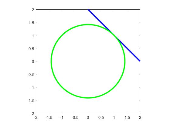
If we look at the equation of the line and rearrange things, we get an equation of x+y=2. If we go back to the Calculus 3 method, we'll get that Fx = 2x, Fy = 2y, so that our gradient is (2,2). Plugging this in to the equation for the tangent line, we get that 2(x-1) + 2*(y-1) = 0 or 2x + 2y = 4, which is equivalent to the equation we had in the Calculus 1 method.
Optimization is a similar process to what was done in Calculus 1. We need to take our function, take all derivatives, and find all points where all of the derivatives vanish. The Lagrange multiplier part of optimization is also similar, take all derivatives, set up the appropriate equations, and solve them simultaneously. In order to do this, we need to use symbolic expressions to solve these problems. For instance, if we already define variables syms x y z and functions f, g of them (note: you will need 4 variables to do this for this lab, but this will give you the idea), we can take all derivatives with
Dfx = diff(f,x);
Dfy = diff(f,y);
Dfz = diff(f,z);
Dgx = diff(g,x);
Dgy = diff(g,y);
Dgz = diff(g,z);
In order to find critical points of f, we then want to solve
Dfx = 0, Dfy = 0, Dfz = 0
and for the Lagrange multiplier part, we need a new variable syms L (for lambda) and want to solve
Dfx = L*Dgx, Dfy = L*Dgy, Dfz = L*Dgz, g = 1
In both of these cases, we need to simultaneously solve a system of equations. Thankfully, MATLAB has an easy way to handle that.
So, we have a collection of equations that we need to solve. MATLAB has a solve command that lets us do just that. If we want to solve the critical point part of the problem, we can write this in the form
[xSols, ySols, zSols] = solve([Dfx == 0, Dfy == 0, Dfz == 0], [x,y,z], 'Real', 'true');
For this command, the first argument is a list of the equations you want to solve, and the second is a list of the variables you want to solve for. As an output from this function, we put the same number of things as we have variables we want to solve for. When we run this command, each of the xSols, ySols, and zSols will be column vectors containing all possible solutions to this system. The last two arguments in the function call just make sure that all solutions are real-valued. This is more likely to be an issue in the Lagrange multiplier case, but you might as well add it in here.
The Lagrange multiplier problem can be solved in the same way,
[LSols2, xSols2, ySols2, zSols2] = solve([Dfx == L*Dgx, Dfy == L*Dgy, Dfz == L*Dgz, g == 1], [L,x,y,z]);
and then we can do things with the solutions. Here, instead of using the ('Real', true) part of the code, we are better off just assuming that L is real. Since x, y, and z will need to be real in order to make g = 1, we only need to add this assumption to L. This can be done by, immediately after declaring L as a sympbolic variable, writing
assume(L, 'real');
I initially tried to run this with the ('Real', true) code, and ran into some problems where MATLAB didn't think that the roots of some sixth order polynomial were real, even though they are. Using this method will circumvent that problem.
Once we have these solutions, we need to determine if the critical points lie in the admissible region and figure out which of the possible extrema are the largest and smallest. We already have the possible x, y, and z values stored in solution arrays (be careful that you don't lose your first points when you get the Lagrange multiplier ones) and just need to plug them in to the functions f and g. We can do this with the subs function as mentioned before. For instance,
val = subs(g, [x,y,z], [xSols(1), ySols(1), zSols(1)]);
will plug the first values from the critical point solver to see what the value of g is at that point. For all of the critical points, you'll need to evaluate g at each of them to determine if the value is less than 1. After that, you will then need to do the same evaluation for f to get the set of possible maximum and minimum values.
In a similar way to the triangle plotting from Lab 1, we could do this a little more effectively by building a matrix of the xSols, ySols, and zSols and then using M(1,:) as the last argument in the subs function.
The idea of the lab from here is fairly straight-forward.
If you want, you are more than welcome to hard-code these answers into your script. That is, run the code to determine the value of g at each critical point. Then, in a comment, write what this tells you about the admissibility of these points, then make a new list that just contains the admissible points. Then you can move on to work on the Lagrange multiplier part, and do the same, evaluating f at each of the points, and then writing in a comment what the maximum and minimum are. However, there is a way to do this entirely in a MATLAB script, but it is a little more tricky. The next sections will walk through what you need to do it this way.
The issue that makes this problem tricky to solve is the fact that we don't know in advance that any or all of the critical points of f will be admissible. We can't just plug all of the critical points into f, because then we may not get the appropriate maximum or minimum. Thus, we need to be a bit more fancy with the code to make this work.
The idea of this trick is to create two additional variables, viablePts, which will end up containing a list of all of the viable points that we want to plug in to f in order to find the maximum or minimum, and nextPt, which will track at what index we need to add our next viable point. You'll want to start your code with
viablePts = zeros(3, 1);
nextPt = 1;
The zeros command generates a column vector of 3 zeros, and the next place we want to put a viable point is the first index. Note: For this sample, I am assuming there are 3 variables. For your problem, there will be 4, so you'll need to adjust as necessary. Next, go through the normal work to generate all possible critical points of f. We now want to loop through all of them to determine which are admissible. This is where we want to use the looping technique discussed in the Lab 0 material:
for count = 1:length(xSols)
Then, we want to check if g at that solution is at most 1, and if it is, we add the point to the list of viable points. Thus, we evaluate g and store it in val, (where we replace the 1 by count) and
if val <= 1
viablePts(1, nextPt) = xSols(count);
viablePts(2, nextPt) = ySols(count);
viablePts(3, nextPt) = zSols(count);
nextPt = nextPt + 1;
end
The point here is, if the value is admissible, we store the x, y, and z values into the list of viable points, and then add 1 to nextPt so that we know where to put the next viable point. After that for loop, we can then go on to finding the set of points from Lagrange multipliers, and all of these can be added to the set of viable points in the same way as above. The code should loop through all of these solutions, and put all of them into the viable points list.
Once that is done, we can then create a list fVals of the values of f at all of the viable points. That is
for count = 1:length(viablePts(1,:))
fVals(count) = subs(f, [x,y,z], viablePts(:,count));
end
Now, we just need to find the largest and smallest values, as well as where they happen.
Thankfully, MATLAB, makes that easy for us to do. We can just write
maxVal = max(fVals)
and
minVal = min(fVals)
which will give us the largest and smallest values in fVals. However, we want more information than that. If we take two arguments out of max or min, MATLAB will also give us the index where the maximum or minimum occurs. Thus, something like
[maxVal, maxInd] = max(fVals)
will put, in maxVal the largest value in fVals, and in maxInd the index where this occurs, so that viablePts(:, maxInd) will contain the x, y and z coordinates of the point where the maximum value of f occurs. The same happens for min. You can use this fact to finish up with the script and displaying the coordinates of the maximum and minimum values of f on the admissible region.
Earlier in Lab 0, we talked about doing integrals. This problem deals with double and triple integrals. In order to do these in MATLAB, we need to write them as iterated integrals. Thus, if we have a symbolic function f(x,y) and want to integrate it over the square [-1,1] × [-1,1], we can write this as
int(int(f, x, -1, 1), y, -1, 1);
and if we wanted to integrate over the triangle 0 ≤ x ≤ y ≤ 1, we can do this by
int(int(f, x, 0, y), y, 0, 1);
For these problems, you will likely have more success if you do a little bit of work by hand to figure out the best way to do these integrals before you try to code them into MATLAB. The same holds for triple integrals.
For computing the center of mass, you should refer to the background data sheet. You will just need to plug the appropriate fomula for f into the integral computations above to get the needed values. Following the formulas on the sheet will let you compute the center of mass.
While it might seem strange, the easiest way to draw and fill in the two-dimensional region is by using the fill command. This fills in the polygon given by the set of vertices you give it. We used this for Lab 1, but if we put in a lot of vertices, the polygon will basically look like the curve. The other key to doing this easily is the fliplr command, which takes in a vector and reverses the order. For example,
fliplr([1,2,3])
3, 2, 1
In order to fill in the polygon, we need to start on the left side, trace one curve from left to right, get to the right endpoint, and trace the second curve backwards from right to left. First, you need to find the endpoints of this region, which I have stored in Lend and Rend. This should be done using the solve command as done before. Remember, you'll want to make sure you only get the real valued solutions of this equality to get the endpoints. You will only get two valid solutions.
Once you have these endpoints, you can plot the region using the following set of commands
xVals = linspace(Lend, Rend, 100);
xDraw = [x, fliplr(x)];
yDraw = [double(L(xVals)), fliplr(double(p(xVals)))];
figure(1);
plot(xVals, double(L(xVals)));
plot(xVals, double(p(xVals)));
fill(xDraw, yDraw, 'r');
which, for a sample pair of functions, will give the following picture.

In order to sketch surfaces and regions in three dimensions, the best bet is to use fimplicit3. This will allow you to specify plot ranges for x, y, and z which will allow you to fine tune the plots to look exactly like you want. If you have the function z = f(x,y), then you can write
fimplicit3(z - f(x,y), [-2, 2, -3, 3, -4, 4])
to plot this surface on -2 ≤ x ≤ 2, -3 ≤ y ≤ 3, -4 ≤ z ≤ 4. This function takes whatever expression you put in and plots the surface where it is zero.
What you'll want to do for this part of the problem is draw both surfaces in the same way, figure out where they intersect (for what z value), and use that to cut off each of the surfaces. For instance, if you want to plot the sphere of radius 1, but only above z = 0.4, you could do this by
syms x y z;
fimplicit3(x^2 + y^2 + z^2 - 1, [-1, 1, -1, 1, 0.4, 1]);
axis([-1.5, 1.5, -1.5, 1.5, -1.5, 1.5])'
which will generate the image
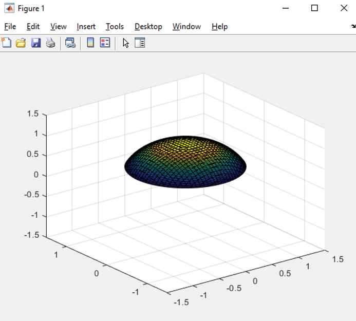
The axis command above has MATLAB make the bounding area of the graph a certain size instead of defining it automatically. Try running these commands without the axis line and see what happens. You can do this with both of the surfaces you need to plot, and then plot both of them on the same axes with hold on; in order to sketch the full region.
For the three dimensional problem, cylindrical coordinates will be useful. However, MATLAB doesn't have a built-in feature for doing polar coordinates. In order to do this, you'll need to work out the change of variables by hand, and then just integrate in r and theta, for instance. To do this, we also need to have r and theta declared as symbolic variables. For example, if you wanted to integrate f(x,y) = x + 2y over the circle of radius 1 centered at (0,0), we can write that as
int(int((r*cos(theta) + 2*r*cos(theta))*r, r, 0, 1), theta, 0, 2*pi);
You can also do things with subs to make it simpler
g = subs(f, [x,y], [r*cos(theta), r*sin(theta)])
int(int(g*r, r, 0, 1), theta, 0, 2*pi)
Notice that we had to explicitly write the r in the integral for the change of variables to polar coordinates. You will need to do the same in this problem for cylindrical or spherical coordinates.