Almost every aspect of the practice of mathematics, both pure and applied, has been improved and amplified in recent decades by the widespread availability of "computer algebra systems", CAS. This technology is much more than just algebra, of course. It is a collection of systematic and powerful programs that permit algebraic manipulation
and numerical approximation
and graphing
The freedom to work with "exact" symbolic computation, with numerical approximation (with specified accuracy) and with visual display of data (human beings learn much more from pictures than from lists of numbers!) is very useful. Maple provides an environment which allows all of these, plus the freedom to move among these representations of mathematical ideas.
Much teaching and research is now improved by access to powerful programs which allow experimentation. Examples can be discovered and explored which are useful for instruction. These programs can also be used to further understand complicated phenomena which are not easily explained.
Many students have graphing calculators. These are useful, but are limited by speed and memory size. Simple errors may occur. There are large computer programs with powerful numerical, symbolic, and graphical capabilities. These still may have the potential for errors (as some of the contents of the link discuss), but much effort has gone into their programming. The most widely distributed programs are Maple and Mathematica These programs are not infallible but they can be very helpful. Other programs are available with special capabilities. For example, Matlab, a program originally directed at problems of linear algebra, is widely used at the Engineering School.
The answers to the questions above were obtained with the following Maple instructions. These instructions are not given to impress you, but rather to show how easy it is to get the answers.
coeff(coeff(coeff((x+y+z)^12,x^6),y^4),z^2);
The command coeff(P,monomial) finds the coefficient of the monomial in the expression P. Layering three repetitions of coeff finds the desired coefficient.
fsolve(3*x+cos(2*x^2)=0,x);
fsolve is a general "floating point" approximate equation solver. Care must be used if there's more than one root. There are also symbolic solvers, useful when there is a nice formula for the solution.
with(plots):
V:=((x^2+y^2)-1):
W:=((x^2+y^2)-2):
implicitplot3d(-V*W=z^2,x=-2..2,y=-2..2,z=-2..2,grid=[30,30,30],axes=normal);
The implicitplot3d command sketches graphs which are defined implicitly by equations. Since Maple has so many functions and libraries available, many need to be specifically loaded before use. The command with(plots); loads a variety of plotting commands. The implicitplot3d command has a wide variety of options. The grid option gives control over the spacing of sample points. Of course increasing the number of sample points "costs" computational time and storage space but does given finer detail.
Other references and programming in
Maple
There's a nice "reference card" with common Maple commands which students may find helpful: please look at this University of Michigan web page.
Maple is also a programming environment. Mapleprograms are called procedures. The Maple language has many statements supporting program flow such as if ...then and while and do etc., and also has a variety of data types. There's no time in this course to teach this material, but students should know that programming is possible.
For guidance on Lab 0, you should follow the PDF file here.
Here is some help for the first Maple assignment. The assignment requests several pictures. Pictures are very important. Not many people can get much information from vast tables of numbers, but humans possess a large capacity to receive and organize visual information. You are allowed, and indeed encouraged, to copy and modify the commands discussed here. Copying and pasting may not transfer the command correctly; you may need to retype them into the Maple window. Remember that all commands should be entered into Maple in one line - this page has some commands broken across two lines because of space limitiations.
Maple has thousands of commands, but many of them are kept in storage in "packages" to save memory. Once Maple is started, you can call up packages via the with command. One package, called plots, contains several three dimensional plotting commands. Enter
with(plots);
in Maple to see a large number of commands appear which are now easily accessible. One of them is spacecurve which will plot three-dimensional parametric curves. To see more about this command you can type
help(spacecurve);
to bring up the help page.
The command
spacecurve([4*t-11,3*t+7,-5*t+2], t=0..1, axes=normal, color=black, thickness=2, labels=[x,y,z]);
draws the parametric function
x = 4t - 11
y = 3t + 7
z = -5t + 2
for the range 0 ≤ t ≤ 1. These equations should give you a line segment from the point (-11,7,2) where t=0, to the point (-7,10,-3) where t=1.
The picture Maple displays (shown above) is deceptive. The line segment is not vertical although it is shown that way. In this case this problem arises because the three coordinate axes are not drawn to the same scale.
Add the "scaling=constrained" option to change the command to
spacecurve([4*t-11,3*t+7,-5*t+2], t=0..1, axes=normal, color=black, thickness=2, labels=[x,y,z], scaling=constrained);
The result is shown below. The
scaling=constrained
makes all the axes have the same scale, and so the line segment is no longer displayed vertically.
The command
spacecurve([3*cos(t)+10,3*sin(t)+4,-3], t=0..Pi, axes=normal, color=black, thickness=2, labels=[x,y,z]);
draws the parametric function
x = 3 cos(t) + 10
y = 3 sin(t) + 4
z = -4
for the range 0 ≤ t ≤ π. (Notice that to get the constant π you need to use the capitalization Pi. Maple treats the words pi and PI as variables.) This should be a semicircle of radius 3 centered at (-10,-4,-3) in the plane z=-3. The view below is unconstrained. The result seems to be a parabolic arc because Maple attempts to stretch the curve to fill up the viewing window as much as possible.
Change the command to
spacecurve([3*cos(t)+10,3*sin(t)+4,-3], t=0..Pi, axes=normal, color=black, thickness=2, labels=[x,y,z], scaling=constrained);
The result is shown below. The curve looks much more like a semicircle.
The image can be manipulated in various ways before "exporting" or printing it. It can be rotated, scaled, etc. with some mouse clicks on the picture.
Often one will want to draw multiple graphs on the same axes for easier comparison. In Maple this is achieved via the display command found in the plots package. Store each graph to its own variable, and then display the set of those variables. For example,
A:=spacecurve([4*t-11,3*t+7,-5*t+2], t=0..1, axes=normal, color=black, thickness=2, labels=[x,y,z], scaling=constrained): B:=spacecurve([3*cos(t)+10,3*sin(t)+4,-3],t=0..Pi, axes=normal, color=black, thickness=2, labels=[x,y,z], scaling=constrained): display({A, B});
The first two commands assign values to the variables A and B. The plots are what get stored to the variables. The display command shows the plots together. As is true with plotting single curves, you'll need to be careful in creating accurate unambiguous graphs. The next section describes some problems to avoid.
We will now show several views of the same pair of curves given above. We show very bad versions of the pictures to emphasize that poor graphs can actually decrease the effectiveness of technical communication instead of helping.
This is the plot with
scaling=unconstrained
.
This is the result with
scaling=constrained
.
Here is a very bad version of the picture. It is taken from "the side", with the x-axis coming straight out of the image. This picture seems to show two line segments, when one of the segments is actually the semicircle viewed edge-on.
Here's another very bad version of the picture. The axes have been taken away, and the viewing angle makes the line segment seem to cross what could be a parabolic arc.
Now we analyze more vectors and show more pictures.
Suppose p is the point (3,10,-7), q is the point (9,8,3), and r is the point (6,5,7). Then we can get the vector from p to q via:
[9,8,3] - [3,10,-7];
[6, -2, 10]
This is the vector from p to q. Notice that square brackets [] are used to represent points/vectors instead of parentheses. A picture of the vector can be created with the spacecurve command. We will store that plot to the variable PQplot.
PQplot:=spacecurve([6*t+3,-2*t+10,10*t-7], t=0..1, axes=normal, color=black, thickness=2, labels=[x,y,z], scaling=constrained);
A similar computation gets the vector from p to r and the corresponding picture:
[6,5,7] - [3,10,-7];
[3, -5, 14]
PRplot:=spacecurve([3*t+3,-5*t+10,14*t-7], t=0..1, axes=normal, color=black, thickness=2, labels=[x,y,z], scaling=constrained);
What about the cross product of the two vectors? The VectorCalculus package has a CrossProduct command with a short version &x. When using the VectorCalculus package, denote vectors via angle brackets < and >.
with(VectorCalculus):
<6,-2,10> &x <3,-5,14 >
22 ex - 54 ey - 24 ez
What are these ex, ey, ez? They are the elementary vectors in the x, y, and z directions, respectively. These are exactly the same as what your book calls i, j, and k. Thus
22 ex -54 ey -24 ez
means the vector < 22, -54, -24 >.
We then can draw the cross product vector as a line segment "based" at p:
CPplot:=spacecurve([22*t+3,-54*t+10,-24*t-7], t=0..1, axes=normal, color=black, thickness=2, labels=[x,y,z], scaling=constrained);
and all three graphs can be displayed with
display3d({PQplot,PRplot,CPplot});
The above picture was rotated so that the cross product vector is more clearly perpendicular to the other two. Other views, such as the one below, are not nearly as clear and should be avoided.
Here is an even worse view: one vector is entirely hidden behind one of the others, making it look like there are only two vectors drawn.
Below is a picture of the triangle in R3 whose vertices are the points p and q and r. This picture is very easy to create using a command in the plots package. Find this command yourself: look at the list of commands in plots, guess, and then use help. A hint: The command you're looking for can do more than triangles. It can also plot quadrilaterals, pentagons, hexagons, and many other two-dimensional shapes in three dimensions.
By the way, by rotating the viewpoint, you can make any of the angles of this triangle seem to be a right angle! Perspective can be misleading and irritating.
Finally, here are the triangle, two of the vectors along the triangle's edges, and the cross product of these two edge vectors. You would also generate this picture via the
display
command. The view has been chosen so that the cross product appears to be perpendicular to the triangle, which it is. Twice the area of the triangle is equal to the length of the cross product.
For this assignment you will need commands from the plots and VectorCalculus packages. Load these packages using the with command, as discussed in Packages section of the Background Information for the first Maple assignment.
We will again be using the spacecurve command from the plots package. For these instructions, we will be using as an example the curve given by:
r(t) = < 5 cos(2t) + 5 sin(t), 2 cos(2t) + 4 cos(t), sin(3t) + 4 sin(t)>
or if you prefer the parametric notation:
x=5 cos(2t) + 5 sin(t)
y=2 cos(2t) + 4 cos(t)
z= sin(3t) + 4 sin(t)
I'm beginning with this curve because it is fairly simple. More complicated curves will appear later. This curve is a closed curve (i.e. a loop) on the interval [0,2π] because the formulas are all combinations of sines and cosines with integers multiplying the parameter, t.
Since we will be doing a lot with this curve, it's wise to store it to a variable. There are several approaches to doing this, but the best for our purposes is storing it as a "live" function, r(t)
r := t -> < 5*cos(2*t) + 5*sin(t), 2*cos(2*t) + 4*cos(t), sin(3*t) + 4*sin(t)>
This should allow us to call r(t) simply by typing r(t), but also evaluate r at a value, say t=2, by typing in r(2). (Another option would have been to store the right hand expression directly to r, omitting the "t ->" portion. In this case we would need to use the subs command to evaluate r at a specific value.)
Let's start by just graphing our curve.
spacecurve(r(t),t=0..2*Pi);
We can use just r(t) because we've already stored the equation to r(t). Notice that we used the capitalization Pi to get the constant 3.141... (pi and PI do not give this constant). The result is the picture shown below.
This picture is not very useful. The rainbow coloration does not add anything and will make the curve fade away if we print out the picture in black and white. It is not clear whether that crossing in the middle is actually a crossing or just an illusion due to the viewpoint. Plus there are no axes to give reference so do not know how far to the left/right, up/down, front/back the curve stretches. Let's add some options to this command to make the picture better. You enter options in the command after the range, separated by commas.
Putting these options into the command we get
spacecurve(r(t),t=0..2*Pi, thickness=2, color=black, axes=normal, labels=[x,y,z], numpoints=150);
Certainly the view shown is much nicer, and has some readable quantitative information (on the axes). It is still a bit deceptive, however, at the center. The picture seems to show the curve intersecting itself. In fact, this particular curve does not have any self-intersections. This is what's called a simple closed curve. If you right-click on a Maple picture, the Manipulator button allows you to rotate or scale or pan. So you can get many different views. Here is a view which shows the same curve from a different angle, and zoomed out farther. Apparently this curve does not intersect itself!
Consider the following picture of the curve, s(t)=< sin(2t), cos(2t), sin(t) >
This shares the a figure-8 shape with our original picture of our curve r(t). This curve actually has an intersection, however, as illustrated by the animation below (created by the animate command - hover your cursor over the animate for the Maple code.)
,cos(2*t),sin(t)>,t=0..2*Pi,color=black,thickness=3,axes=boxed,orientation=[129,phi]], phi=0..360, frames=90)")
Since you cannot print an animation, you should include several views of your curve to convince the reader of any intersections.
Warning: There are curves which do not intersect themselves, but have the irritating (interesting?) property that every two dimensional view shows intersections! See the bottom of this page for examples. For example, q(t)=<sin(t),cos(3t),sin(2t)> (animated below) has this property. In this case you would include several views of your curve to convince the reader that there are no intersections.
,cos(3*t),sin(2*t)>,t=0..2*Pi,color=black,thickness=3,axes=boxed,orientation=[75,phi]], phi=0..360, frames=90)")
Watch as intersections appear and disappear. Compare this to a curve with an actual intersection, such as s(t)=<sin(2t), cos(2t), sin(t)> above where the intersection does not disappear. More examples of such curious curves appear at the bottom of this page.
As there will be several animations in this lab, here are some details on the command.
As an example, say I want to draw a point tracking around the curve r(t) from earlier. We can do this with the following:
with(plots):
C := spacecurve(r(t),t=0..2*Pi, thickness=2, color=black, axes=normal, labels=[x,y,z], numpoints=150):
animate(pointplot3d, [r(t), color = blue, symbol = solidsphere, symbolsize = 30], t = 0 .. 4*Pi, frames = 100, background = C);
Note: If you also want to display the curve on it's own, you should display(C) as well. In the animate command, the background command puts the curve behind the point that is moving, and the symbol and symbolsize options change the moving point to be a sphere that is large enough to see. Since I set the t range in the animate command to be from 0 to 4 pi, the point will trace around the curve twice. Running this code produces the following animation.
We can try various views to get the size of the curve. Two images are shown below (here we used the "axes=frame" option instead of "axes=normal"). The image on the left has the z-axis sticking directly out from the viewing plane, so we are looking down from above. Alternately, you can see this as projecting (i.e. squashing) the curve into the xy-plane. The image on the right has the y-axis sticking directly out from the viewing plane. Therefore it shows a picture of the curve squashed into the xz-plane.
From these pictures I can get a rough idea of the dimensions of this curve. Apparently the curve fits inside a box with -10≤x≤6 and -3≤y≤6 and -3.6≤z≤3.6, as illustrated below. You may draw such markings by hand.
How long is this curve? This is called the arc length, which is calculated by integrating the speed of r(t) for the desired range of t (i.e. ∫ab |r'(t)| dt ). We need to differentiate r(t), and then find its length or magnitude (this is the speed). The diff command will differentiate r(t). The VectorCalculus package contains a command called Norm which computes the norm of a vector. We will use the variable speed to represent |r'(t)|.
speed:=Norm( diff(r(t),t) );
speed:=((-10*sin(2*t)+5*cos(t))^2+(-4*sin(2*t)-4*sin(t))^2+(3*cos(3*t)+4*cos(t))^2)^(1/2)
We are interested in the length of one loop of the curve. For our curve "one loop" is given by the range 0 ≤ t ≤ 2π, so we need to integrate speed from t=0 to t=2*Pi to get the length. We can integrate using the int command, so may naturally try:
int(speed, t=0..2*Pi);
Notice that when you use int here, however, Maple usually returns the original integral, not evaluated, after about 12 seconds' thought. When Maple returns the original command, it means that Maple has given up trying to evaluate whatever you asked. Usually this is because you typed in something that the program does not recognize, but in this case it is because Maple cannot solve this integral symbolically. This is not surprising -- most functions defined by formulas can't be antidifferentiated in terms of familiar functions.
Maple needs to be "convinced" to evaluate this integral approximately. You can do this via:
evalf(Int(speed,t=0..2*Pi));
56.13189562
Please note the capital I in the integrate command. This is an important difference which you can read about on a help page if you want. The numerical computation of the integral took less than a hundredth (.01) of a second. This curve is about 56 units long.
The other main part of this lab is computing an arc length parametrization for the curve. The background file for this lab gives a step-by-step process for doing this.
L := b -> int(speed, t=0..b)
Since speed is defined as an expression in t<\span>, you must use t as the variable of integration. To remedy this, you could either use a subs command to replace t by a new variable, for instance
speed_tau := subs(t=tau, speed) and then you can use tau as the variable of integration. You could also fix this by making speed a function, for instance
speed := t -> subs(a=t, Norm(diff(r(a),a)). Writing this as speed := t -> Norm(diff(r(t),t)) does not work because if you try to evaluate speed at 1, it will try to compute Norm(diff(r(1),1)) and taking the derivative of a number with respect to a number doesn't make sense.
In the first case, Maple realizes that it first needs to take the derivative, then the norm, and finally plug in the value you want. Before you actually define the function L(t) though, it may be important to force Maple to simplify the expression for speed into something that it can actually handle
(this is particularly relevant for the types of functions that you are being given for this assignment. In order to do that, you should write something of the form speedsim := t -> sqrt(factor(simplify(speed(t)^2))) If you look at this expression, you'll see that it does not change the actual value of the function speed. However, by squaring it and letting Maple sort out what the function looks like, you get a better result than you might otherwise.
solve(s = L(t), s)
and then you'll want to save the function that comes out as g(s).
You may get multiple functions here, and that's not too surprising. If your function L(t) is a quadratic polynomial (for example), then you would expect to have two possible solutions/inverses based on where you are in the domain. The main thing you can do to
guarantee that you get the correct solution is to assume that b<\span> (which is the end time of our integration) is positive. We know that it is positive from the fact that our curve goes from t=0 to some positive number. We can do this by writing
assume(b > 0 'real') before defining the function L(b). Then, you can do
g := s -> solve(s = L(b), b, useassumptions=true) which will set g to be the appropriate function. At this point, we can then find r2 by setting
class=code> r2 := s -> r(g(s)) and then display r2 by typing r2(s) in the next line. Aren't you glad you didn't have to do this by hand?
Some strange things can happen. Let me show you a few of them.
Below are three pictures of another curve. I emphasize that these are all pictures of the same curve. This curve does not intersect itself, but every two dimensional view does seem to show an intersection. So detecting intersections by "just looking" may be a bit difficult. Some examination of the images is necessary.
Here are two pictures of yet another closed curve. This closed curve does have two self-intersections, each of which can appear to be an illusion. It can be difficult to convince people of these intersections without much numerical work (e.g. showing that r(t0)=r(t1) for some 0 ≤ t0 < t1 < 2 π) or many carefully chosen pictures. If you have suggestions, please let me know.
What possible two-dimensional pictures can result from such an equation? Here are some examples.
This might be the most disturbing "picture". The equation x2+y2+1=0 is not satisfied by any pairs of numbers, (x,y), since the right-hand side is always positive. (Maybe this is an advertisement for complex numbers?)
Look at 29x2+2xy+10y2+8x+12y+4=0. Then realize this is the same as (5x-y)2+(2x+3y+2)2=0 because (5x-y)2=25x2-10xy+y2 and (2x+3y+2)2=4x2+9y2+4+12xy+8x+12y. I did this in reverse, actually, and started with the squares. But the only way that (5x-y)2+(2x+3y+2)2 can be 0 is if (squares are never negative!) 5x-y=0 and 2x+3y+2=0. The first equation gives y=5x and when substituted in the second equation you get 2x+3(5x)+2=0 so that x=-2/17 and then y=-10/17. So "clearly" (not so clearly to me!) the point (-2/17,-10,17) is the only solution to 29x2+2xy+10y2+8x+12y+4=0.
Just x+y=0 will do.
|
Certainly students should recognize x2+2y2-1=0 as an ellipse. But you may find it difficult to believe that 11x2-32xy+24y2+24x-40y+21=0 is also an ellipse. You could try the Maple command implicitplot(11*x^2-32*x*y+24*y^2+24*x-40*y+21=0, x=1..6, y=2..5, scaling=constrained, thickness=2, color=black, grid=[100,100]); and see the result. Most of the options to this command should be familiar (the thickness and scaling, for example). One option which might be new is grid. The default for the implicit plot command is to check on a 25 by 25 grid (that's 625 points). Requesting more points will usually give a smoother picture. Of course, the grid=[100,100] requires 42=16 times as much computation. On my home PC, the [25,25] grid took about .064 seconds and the [100,100] grid took about .72 seconds. |
With grid=[100,100] |
|---|---|
| |
| No specification, so grid=[25,25] | |
|
|
One simple example is x2+y=0. And, again, it may not be obvious that 25x2-40xy+16y2+13x-9y+3=0 is also a parabola, but displayed to the right is the result of this Maple command: implicitplot(25*x^2-40*x*y+16*y^2+13*x-9*y+3=0, x=-10..0, y=-10..0, scaling=constrained, thickness=2, color=black, grid=[100,100]); |
|
|
The model hyperbolas you have been told about include xy=1 and x2-y2=1. But -7x2-6xy+16y2+48x-80y+74=0 is also the equation of a hyperbola whose graph is shown to the right. |
|
Well, xy=0 is sort of a hyperbola. It is (sigh!) a degenerate hyperbola or limiting form of a hyperbola. For example, xy=0 is a pair of lines which intersect in one point, and this "curve" is certainly the limit of the curves xy=tiny number as tiny number-->0. Also two parallel lines can be described by a quadratic polynomial: the points (x,y) which satisfy x2=1 are the straight lines x=1 and x=-1. This is another "degenerate" case.
All of these curves are called conic sections.
We need to build a right circular cone. This is a cone with a central axis perpendicular to a plane.
Step 1Take a straight line (which will be the axis of symmetry of the cone), and take a plane perpendicular to the line. In the plane, imagine a circle whose center is the point of intersection of the line and the plane. Now fix a point on the line outside of the plane. |
|
Step 2Now draw a straight line through the external point and every point on the circle. This collection of lines will form a surface. Each of the lines is called a generator of the cone. The original line is the axis of symmetry of the cone. The external point is called the vertex of the cone. |
|
| The right circular cone looks like what is sketched to the right. Suppose this cone is sliced by another plane. A conic section is the resulting curve: the intersection of the cone and the plane. The type of the curve is determined by the angle made by the intersecting plane and the axis, and how this angle relates to the vertex angle of the cone. |
|
EllipseIf the angle made by the intersecting plane and the axis is greater than the vertex angle, then the plane will only slice through one of the cone's pieces. The resulting curve is an ellipse. |
|
HyperbolaIf the angle made by the intersecting plane and the axis is less than the vertex angle (or is parallel to the axis of symmetry), then the plane will slice through both parts of the cone's pieces. The resulting curve is a hyperbola. |
|
ParabolaIf the intersecting plane is exactly parallel to one of the generating lines (and that's darn unlikely for a random plane!) then the plane will slice through only one part of the cone. The resulting curve is a parabola. |
|
These geometric characterizations of the conic sections are thousands of years old. There are also definitions of the various conic sections using distance in the plane. For example, an ellipse is the collection of points the sum of whose distances to two fixed points is a constant.
If the universe were empty except for the sun (a heavy point mass) and an asteriod (a much lighter mass) than the orbit the asteroid would have around the sun would be a conic section. The textbook discusses this in the section on Kepler's laws. So these curves (motion in an inverse square law force field) will be everywhere in physics.
Suppose we want to know which conic section is given by Ax2+Bxy+Cy2+Dx+Ey+F=0. I'll assume that |A|+|B|+|C|>0, so that at least one of the quadratic coefficients is not 0. Otherwise we've just got a line or a point. The type of the curve depends on the discriminant. The discriminant is defined to be B2-4AC.
We looked at the ellipse 11x2-32xy+24y2+24x-40y+21=0 earlier, with A=11, B=-32, and C=24. The (-32)2-4(11)(24) turns out to be -32.
An example of a hyperbola earlier was -7x2-6xy+16y2+48x-80y+74=0. Here A=-7, B=-6, and C=16, so B2-4AC=(-6)2-4(-7)(16)=484>0.
I had claimed earlier that 25x2-40xy+16y2+13x-9y+3=0 was a parabola. Here (-40)2-4(25)(16)=0.
These algebraic statements are several hundred years also, and can be verified using high school algebra, but the "high school algebra" must be applied very diligently. Some students might see a resemblance in the discriminant analysis and consequences to the second derivative test for functions of two variables, and the resemblance is not accidental. The second derivative test actually uses these results in a somewhat disguised form, where the Ax2+Bxy+Cy2+Dx+Ey+F is the second order Taylor polynomial of the function.
Let's start with a random function, say F(x,y,z)=x3+5xz-y3+y. Your function will have highest degree 2, so it'll be different from this one, but we can work from this. The point (1,0,0) is on the level surface F(x,y,z)=1. The gradient vector is perpendicular to the tangent plane to this level surface, as described in the background document. First, we should store the function and verify that (1,0,0) is on the level surface.
F:=x^3+5*x*z-y^3+y;
F:= x3 + 5xz - y3+y
subs({x=1, y=0, z=0}, F);
1
Next, we need to find the gradient of F and evaluate it at the point (1,0,0).
Fx:=diff(F,x);
Fx := 3x2 + 5z
Fy := diff(F,y);
Fy := -3y2 + 1
Fz:=diff(F,z);
Fz := 5x
subs({x=1,y=0,z=0},Fx);
3
subs({x=1,y=0,z=0},Fy);
1
subs({x=1,y=0,z=0},Fz);
5
Therefore, the gradient of F at (1,0,0) is (3,1,5). Thus, the command
T:=spacecurve(<3*t+1,1*t,5*t>,t=0..(.3),color=blue,thickness=3, axes=normal);
would draw the normal vector to this surface going through the point (1,0,0). However, that's not quite what we want here. We want a tangent plane, which, by how the equation of planes are written, has the form 3(x-1) + 1(y-0) + 5(z-0) = 0 or 3x + y + 5z = 3. Since we want this plot to touch the graph of the surface at (1,0,0), we can draw this plot as an implicitplot3d command:
TP := implicitplot3d(3*x+y+5*z = 3, x = .4 .. 1.6, y = -.6 .. .6, z = -.6 .. .6, axes = normal, labels = [x, y, z], grid = [10, 10, 10], color = blue, style = surface):
We can also draw the surface by
S := implicitplot3d(F = 1, x = -2 .. 2, y = -2 .. 2, z = -2 .. 2, axes = normal, labels = [x, y, z], grid = [50, 50, 50], color = red, style = surface):
and then display both of them by
display({S,TP});
Specifying that grid=[50,50,50] means that we should get a better picture than the default, but Maple must check 503=125,000 points in R3 and this command took about 2 seconds on my home PC.
Below is the picture that resulted from displaying the tangent plane and the piece of the surface together.
What if I wanted to find the normal vector for some point that isn't as "nice" as (1,0,0)? Suppose I changed x, say, from 1 to .95, and z from 0 to -.15. What y values could I get? Here's one way to have Maple approximate the answers.
The first step here finds the y-coordinate that is on the surface and has x-coordinate 0.95 and z-coordinate -0.15. You'll want to run something similar to this for your code. It is entirely possible (and will happen for your code) that you could get more than one solution here. In that case, you'll want to save more than one point to a variable like we did for Q here.
fsolve(subs({x=.95,z=-.15},F=1));
-1.289608097
Q:={x=.95,y=-1.289608097,z=-.15};
Q := {x = 0.95, z = -0.15, y = -1.289608097}
The point of saving Q like this here is so that we don't have to type as much later. Think about what the code would look like if you didn't save Q, particularly in the subs commands below. Now, we verify that Q is on the surface F=1.
subs(Q,F);
1.000000000
In order to draw the tangent plane, we need to find the normal vector at this point. We already have the gradient of F stored as Fx, Fy, Fz, so we just need to plug Q into these expressions. For ease of use later, we also store these in variables.
m1:=subs(Q,Fx); m2:=subs(Q,Fy); m3:=subs(Q,Fz);
m1 := 1.9575
m2 := -3.989267132
m3 := 4.75
Finally, we want to draw the tangent plane and add it to our previous plot.
TP2 := implicitplot3d(m1*(x-.95)+m2*(y+1.289608097)+m3*(z+.15) = 0, x = .4 .. 1.6, y = -1.9 .. -.7, z = -.7 .. .5, color = green, style = surface, axes = normal):
display({S,TP,TP2});
In the drawing command above, I just picked a small window around the point Q on which to draw the plane. It doesn't have to be symmetric around the point, so long as it contains Q. If it doesn't look like the planes are tangent to the surface, try rotating the picture to get a better view of it.
|
|
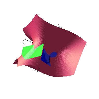
For curves, the process is very similar, but our `tangent plane' is really just a `tangent line' because it is only one dimensional. The steps you follow are all symmetric. Again, we will use a function F here that is more complicated and strange than the ones you will be dealing with, but the work is all the same.
F:=x^5-3*x*y^2+4*x+2*y;
F := x5- 3 x y2+ 4 x+ 2 y
subs({x=1,y=2},F);
-3
Fx:=diff(F,x);Fy:=diff(F,y);
Fx := 5 x4 - 3 y2 + 4
Fy := -6 x y + 2
m1:=subs({x=1,y=2},Fx); m2:=subs({x=1,y=2},Fy);
m1 := -3
m2 := -10
TL:=implicitplot(m1*(x-1) + m2*(y-2) = 0, x=0.5..1.5, y=1.5..2.5, color=blue, thickness=2);
S2:=implicitplot(F=-3, x=-5..5,y=-5..5, thickness=2, scaling=constrained, color=red, grid=[50,50]);
display({S2,TL});
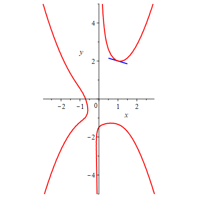
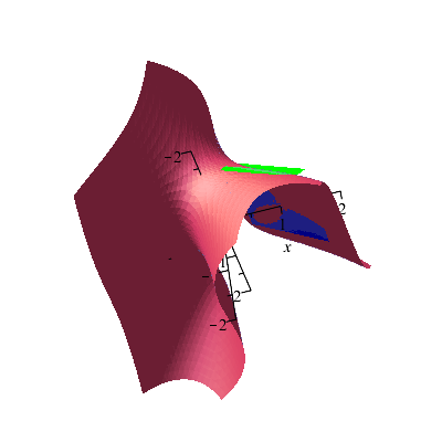
Look at the picture. If x=-1.72, there are two values of y which will put (-1.72,y) on the curve. Maple can approximate these values, and then it can find and graph representations of the normal vectors at these points.
fsolve(subs(x=-1.72,F=-3));
-2.119122494, 1.731525595
Q1:={x = -1.72, y = -2.119122494}; Q2:={x = -1.72, y = 1.731525595};
Q1 := {x = -1.72, y = -2.119122494}
Q2 := {x = -1.72, y = 1.731525595}
y1 := -2.119122494; y2:= 1.731525595;
y1 := -2.119122494
y2 := 1.731525595
mx1:=subs(Q1,Fx); my1:=subs(Q1,Fy); mx2:=subs(Q2,Fx); my2:=subs(Q2,Fy);
mx1 := 34.28861236
my1 := -19.86934413
mx2 := 38.76611014
my2 := 19.86934414
TL1 := implicitplot(mx1*(x+1.72)+my1*(y-y1) = 0, x = -2.4 .. -1.0, y = y1-1 .. y1+1, color = green, thickness = 2):
TL2 := implicitplot(mx2*(x+1.72)+my2*(y-y2) = 0, x = -2.4 .. -1.0, y = y2-1 .. y2+1, color = purple, thickness = 2):
display({S2,TL,TL1,TL2});
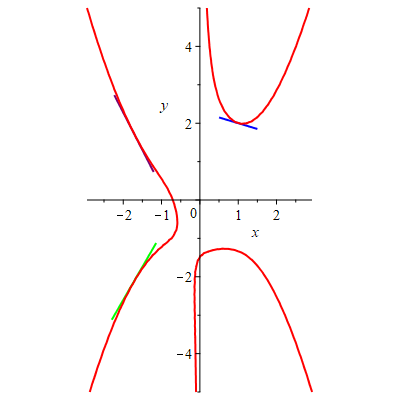
Note: In getting the picture to look good, you may need to play with the different parameters for how big the surface is, how long each of the tangent lines are, and the grid sizes. It shouldn't take too much time to get something that looks decent.
You may be thinking at this point, didn't we do tangent lines in Calculus 1? Why can't we just use that method to find these tangent lines? The answer is you can, but the method here is more general. Consider the function F(x,y) = x^2 + y^2. The graph of F = 2 is a circle. However, we can't describe this as y = f(x) because the graph doesn't pass the vertical line test. We can see this explicitly in Maple when we try to solve for y.
F:= x^2 + y^2:
solve(F=2, y);

There are two different functions here, and if you draw them, you can see that one does the top half of the circle, while the other does the bottom. If we split it this way, then each one individually passes the vertical line test. Now, let's say we want to find the tangent line at (1,1), which is on the curve defined by F = 2. We want to use the first of the two functions because it has a positive sign, and if I plug in x=1, I get that y=1 as well. For the other function, I would get y=-1, so that is not the equation that I want.
From that equation, we can then do use normal Calculus 1 techniques to find the tangent line.
f:= sqrt(-x^2 + 2);

fx := diff(f,x);

m := subs(x=1, fx);
m:=-1
TL := plot(m*(x-1)+1, x=0..2, color=blue, thickness=2):
Cir := implicitplot(F = 2, x=-2..2, y=-2..2, color=green, thickness=2):
display({Cir,TL});

If we look at the equation of the line and rearrange things, we get an equation of x+y=2. If we go back to the Calculus 3 method, we'll get that Fx = 2x, Fy = 2y, so that our gradient is (2,2). Plugging this in to the equation for the tangent line, we get that 2(x-1) + 2*(y-1) = 0 or 2x + 2y = 4, which is equivalent to the equation we had in the Calculus 1 method.
Here is the problem:
Theoretical results imply that the function f(x,y,z) = x2+x+3yz has a maximum and a minimum on the (solid) ball defined by g(x,y,z) = x2+y2+z2 ≤ 1. Find these maximum and minimum values by
We first discuss the problem of finding critical points of the objective function and determining whether or not they are relevant to our problem. A critical point of f(x,y,z) is determined by the condition ∇f(x,y,z) = 0. Since our objective function is quadratic the resulting equations will be linear and will have a unique solution (or, in general, possibly an infinite number of solutions, but the latter case will not occur for data in this lab). In our example ∇f(x,y,z) = <2x+1,3z,3y>, so that the equations to be solved are 2x+1 = 0, 3z = 0, and 3y = 0.
Here is one way to get Maple to solve these (rather trivial, in this example) equations and to test the resulting critical point.
f:=x^2+x+3*y*z;
f := x2 + x + 3 y z
g:=x^2+y^2+z^2;
g := x2 + y2 + z2
CPeqx:=diff(f,x)=0;
CPeqx := 2 x + 1 = 0
CPeqy:=diff(f,y)=0;
CPeqy := 3 z = 0
CPeqz:=diff(f,z)=0;
CPeqz := 3 y = 0
CPsol:=solve({CPeqx,CPeqy,CPeqz});
CPsol := { x = -1/2, y = 0, z = 0 }
CPgvalue:=subs(CPsol,g);
CPgvalue := 1/4
CPfvalue:=subs(CPsol,f);
CPfvalue := -1/4
The command CPeqx:=diff(f,x)=0 labels
the equation ∂ f / ∂ x = 0
as CPeqx so that it can be referred to
later. The = is part of an equation,
and the symbols := are used by Maple to assign a value. In this case, the "label"
CPeqx is assigned as its value the
equation diff(f,x)=0.
The solve
step finds all solutions of the system of equations (in this case there is only one such solution). Finally, the commands
CPgvalue:=...
and
CPfvalue:=...
substitute the critical point into the constraint and objective functions.
In this case, because the value of g at the critical point is less than 1, the critical point lies inside the domain of interest, and CPfvalue is a candidate for an extreme value of the objective function.
The boundary of our region of interest is the surface g(x,y,z)= x2+y2+z2=1, a sphere which easy to understand and to visualize. The objective function f(x,y,z)=x2+x+3yz may take its maximum value, its minimum value, or both on this surface, and points at which this can happen may be found by the method of Lagrange multipliers.
To appreciate the method of Lagrange multipliers it is helpful to visualize the constraint surface together with surfaces on which the objective function is constant: f(x,y,z) = C. The first picture on the right shows the sphere together with the surface on which f = C with C = 1; the latter surface is a hyperboloid of one sheet. The choice C = 1 is not significant here; it shows a typical situation. The hyperboloid divides the sphere into two pieces. On one piece of the sphere, the function f(x,y,z) has values larger than 1, and on the other piece the values of the function are less than 1. Clearly 1 is not an extreme value.
The second picture shows the sphere together with the surface f(x,y,z) = 2 (again a hyperboloid of one sheet). Now the hyperboloid does not cut the sphere into two pieces; it just touches it tangentially at a single point. The value of f(x,y,z) at any points other than that point of tangency must be less than 2, so that 2 must be the maximum value of f(x,y,z) on the sphere.
The first picture above was drawn with the following Maple commands (similar commands were used for the second picture and other pictures below):
pg:=implicitplot3d(x^2+y^2+z^2=1,x=-2..2,y=-2..2,z=-2..2,axes=none,numpoints=1800,color=blue): p1:=implicitplot3d(x2+x+3*y*z=.5,x=-2..2,y=-2..2,z=-2..2,axes=none,numpoints=1800,color=green); pt1:=textplot3d([-1.0,2.5,-2,typeset(f(x,y,z)=1)],font=[Helvetica,16],axes=none): display3d(pg,p1,pt1,orientation=[50,20,0]);
Here the
implicitplot3d
commands create the pictures of the two surfaces, the
textplot3d
command creates the label giving the value of C, and the
display3d
command combines these into the final picture. The numpoints=1800 option increases the number of points sampled from the default of 1000. With only 1000 points, the graphs drawn for the surfaces look very polyhedral—that is, they resemble more closely linear approximations to the true smooth graphs. The orientation option specifies the point of view; it corresponds to angles ϑ = 50, φ = 20, and ψ = 0.
Consider again the surface f(x,y,z)=x2+x+3y = C and its intersection with the constraint surface, the sphere g(x,y,z)=x2+y2+z2=1. As discussed above, if the surfaces are not tangent at an intersection point (such surfaces are called transverse) then there will be values of f greater and less than C on the constraint surface, but this will not happen (or more precisely, may not happen) if the surfaces are tangent. The Lagrange multiplier equations follow from this observation: we look for extreme values among the solutions x, y, and z of the equations
∇f(x,y,z)=λ∇g(x,y,z)
Here λ is a real number, and the equality indicates that the tangent planes are parallel because the normal vectors are pointing in the same direction. This one vector equation is three scalar equations.
g(x,y,z)=1
This guarantees that the solutions we seek will be on the constraint surface.
In this specific case, we want to solve these equations
2x+1= λ(2x) 3z=λ(2y) 3y=λ(2z) 1=x2+y2+z2
Here is one way to get solutions, assuming that Maple has already been given the functions f and g. The first command instructs Maple to consider only real numbers in solving the Lagrange multiplier equations; the need for this command is discussed further under "A cautionary example" below.
with(RealDomain):
LMeqx:=diff(f,x)=L*diff(g,x);
LMeqx := 2 x + 1 = 2 L x
LMeqy:=diff(f,y)=L*diff(g,y);
LMeqy := 3 z = 2 L y
LMeqz:=diff(f,z)=L*diff(g,z);
LMeqz := 3 y = 2 L z
LMsols:=solve({LMeqx,LMeqy,LMeqz,g=1});
LMsols := { L = 3/2, x = 1, y = 0, z = 0 },
{ L = 1/2, x = -1, y = 0, z = 0 },
{ L = -3/2, x = -1/5, y = -2 √3 / 5, z = 2 √3 / 5 },
{ L = -3/2, x = -1/5, y = -2 √3 / 5, z = 2 √3 / 5 }
LMvalues:=seq(subs(LMsols[j],f),j=1..nops({LMsols}));
LMvalues := 2, 0, -8/5, -8/5
The commands here are similar to those used above to find the critical point of f, and we comment only on what is new. L is used instead of λ. The Lagrange multiplier equations in this example have four solutions; the solve step finds all the solutions. Finally, the command
LMvalues:=...
substitutes the values found into the objective function. Inside, the
nops({LMsols})
instructs Maple to count the number of elements in the set of solutions -- that is, the number of solutions to the Lagrange multiplier equations. Then Maple will substitute each of these solutions, in order, into the objective function.
From the above we have learned that the maximum value of the objective function on the sphere is 2, and this is attained at the point (1,0,0). The minimum value is –8/5, attained at the two points (−1/5,−;2√3/5, 2√3/5) and (−;1/5,2√3/5,−;2√3/5). The value f(x,y,z) = 0 is obtained from one solution of the Lagrange multiplier equations but does not correspond to either a maximum or a minimum of the objective function.
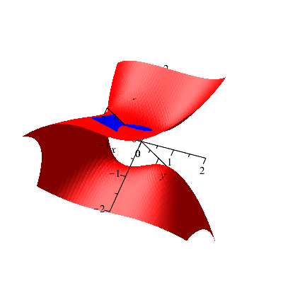
The graph on the right shows a close-up picture of the point of tangency between the sphere and the surface f(x,y,z) = 0. (This is not quite true, because the picture was actually obtained from the objective function x+3xy, but this makes no essential difference.) One can see there how the two surfaces have a point of tangency as well as points where they cross transversely. The objective function, restricted to the surface of the sphere, has a saddle behavior.
Our analysis of the critical point gave us one candidate for an extreme value of f(x,y,z) in the domain g(x,y,z) ≤ 1; this was the value −1/4 at the critical point itself. The Lagrange multiplier equations gave us three candidate values:
2, 0, and −8/5,
By inspection of these four values we conclude that the maximum value is 2 and the minimum is −8/5. If the critical point had not fallen inside the domain g ≤ 1 then we would have had to consider only the values from the Lagrange multiplier analysis.
Students working by hand frequently discard two of the solutions found by Maple. These are the solutions with y=0 and z=0 -- perhaps these are thought to be "trivial" solutions which can't give useful answers. Such solutions should not be thrown away. For the objective function x+3xy these solutions are not extreme values but are more complicated.
Suppose we keep the unit sphere x2+y2+z2=1 as constraint, and consider the objective function F(x,y,z)=x+0.5yz. What follows is true for F(x,y,z)=x+kyz if 0≤k≤1, but keeping track of the results for one value of k will be complicated enough!
The maximum value of this F on the unit sphere is 1, and this value occurs only at the point (1,0,0). The minimum value is −1, which occurs only at the point (−1,0,0). A picture of the constraint surface and the level surface of the objective function which corresponds to the maximum value, the graph of x+0.5yz=1, is shown to the right.
Algebraically, this is a solution to the Lagrange multiplier equations which has both y=0 and z=0. This sort of solution is exactly one which may be thrown away when people compute "by hand".
Here is a sequence of Maple commands similar to those above done. We only display the results of the last command. This should give the values of the objective function which result. The extreme values should be among these "candidates".
F:=x+0.5*y*z:
g:=x^2+y^2+z^2:
LMeqx:=diff(F,x)=L*diff(g,x):
LMeqy:=diff(F,y)=L*diff(g,y):
LMeqz:=diff(F,z)=L*diff(g,z):
LMsols:=solve({LMeqx,LMeqy,LMeqz,g=1}):
LMvalues:=seq(subs(LMsols[j],x+.5*y*z),j=1..nops({LMsols}));
LMvalues := {1., -1., 1.250000000, 1.250000000, -1.250000000, -1.250000000}
The values which Maple returns as
candidates for extreme values are ±1 and ±1.25.
To the right is a graph of the unit sphere and the surface x+0.5yz=1.25, at an angle similar to what was just shown before. The surface for the candidate "extreme value" does not seem to touch the unit sphere! What happened?
Let's show a bit more information about by looking in detail at the result of one of the intermediate steps, the solve command.
> LMsols:=solve({LMeqx,LMeqy,LMeqz,g=1});
LMsols := {z = 0., x = 1., y = 0., L = 0.5000000000},
{z = 0., y = 0., x = -1., L = -0.5000000000},
{x = 2., L = 0.2500000000, z = 1.224744871 I, y = 1.224744871 I},
{x = 2., L = 0.2500000000, z = -1.224744871 I, y = -1.224744871 I},
{x = -2., z = 1.224744871 I, y = -1.224744871 I, L = -0.2500000000},
{x = -2., y = 1.224744871 I, z = -1.224744871 I, L = -0.2500000000}
The third element of LMsols is
{x = 2., L = 0.2500000000, z = 1.224744871 I, y = 1.224744871 I}
where I is Maple's notation for i, or the square root of −1. If we compute
2.+.5* 1.224744871 I* 1.224744871 I
(that's x+.5yz at this "point") then the result, to 10 digit accuracy, will be 1.250000000.
Here is a quote from a Maple help page. It is an important part of the design of Maple which should be known to every user:
By default, Maple performs computations under the assumption that the underlying number system is the complex field.
So, for example, we have:
solve(x^2+1);
I, -I
The Maple command with(RealDomain), which we introduced above, changes this default setting. In the case of computations with Lagrange multipliers such a change is useful. Consider the following commands and responses.
with(RealDomain):
solve(x^2+1);
LMsols:=solve({eqx,eqy,eqz,g=1});
LMsols := {z = 0., x = 1., y = 0., L = 0.5000000000},
{z = 0., y = 0., x = -1., L = -0.5000000000}
values:=seq(subs(LMsols[j],x+.5*y*z),j=1..nops({LMsols}));
values := 1., -1.
When the RealDomain package is loaded, Maple declares that x2+1=0 has no roots. It also discards any elements LMsols which have non-zero imaginary parts, and so it declares as a result of the substitution step, only those values which correspond to real solutions of the Lagrange multiplier equations. We don't get the outputs ±1.25 because the intermediate steps involved imaginary numbers which RealDomain discards. Those solutions won't be geometrically valid.
Integration in more than one dimension can pose difficulties which are new and unexpected compared to similar problems in one dimension. Certainly visualization of the regions can be difficult, and even numerical approximation of definite integrals can be computationally much lengthier (grid points go up as n3 in R3, after all!). Some sample problems are discussed here.
Unfortunately and quite strangely, Maple does not have a built-in command to plot the region between two curves. There is a an option (filled=true) which will shade the region between a curve and the x-axis, but that is the extent of filling options. Hence we need to implement a slightly awkward work-around.
We begin with something simple. The parabola y=x2 and the line y=2x+3 intersect at the points (-1,1) and (3,9). You can use
solve(x2 = 2*x+3, x)
(or similarly with fsolve) for these intersection points. The left-hand picture below shows the boundary curves of the region, drawn with the command
plot({x^2,2*x+3},x=-2..4,thickness=2,scaling=constrained)
To plot the region between the curves, we will use
plot3d
to plot the plane z=0. We will not plot all of it, however. We will only plot the piece of z=0 bounded by the equations y=x2 and y=2x+3. We will set the orientation so that the initial view will an aerial view, making the region look like a two-dimensional plot.
plot3d(0, x=-1..3, y=x^2..(2*x+3), scaling=constrained, axes=normal, color=blue, style=patchnogrid, orientation=[-90,0])
If you play with orienation of the image, you will see what we are really plotting:
The choice between whether to use constrained or unconstrained scaling is up to the user. The choice should be made with the goal of effective visual communication in mind. You may wish to try both views in this and in other plotting situations, and choose which one seems best in the specific situation. This assignment commonly generates regions which are very tall and thin, which do not look good when scaling=constrained is used.
We can compute the area of the region with either a single or a double integral. A single integral which gives the area is in the tradition of "Calc 1".
int((2*x+3)-x^2,x=-1..3);
32/3
We can also compute area via a double integral of 1dA as you learned in Chapter 15.To do a double integral, simply use one int command inside another.
area:=int( int(1, y=x^2..(2*x+3)), x=-1..3);
area:=32/3
Notice how the ranges for the integrals are the same as the ranges when we plotted the region. This is not a coincidence.
Suppose we think of the region enclosed by these two curves as a flat metal plate with constant density (what the text calls a lamina, see section 15.5). In fact, let's assume that the density is 1. Then the total moment of the lamina around the x-axis is given by taking the double integral of y over the region.
x_moment:=int(int(y,y=x^2..2*x+3),x=-1..3);
x_moment := 544/15
Similarly, the total moment around the y-axis is the double integral of x over the region:
y_moment:=int(int(x,y=x^2..2*x+3),x=-1..3);
y_moment := 32/3
Then the center of gravity (here, due to the constant density, this is sometimes called the centroid) is given by "averaging" with respect to the total area:
centroid:=[y_moment/area,x_moment/area];
centroid := [1, 17/5]
We should then be able to balance the region on the tip of a finger at this point. You could try to "build" a region out of cardboard. Then you should be able to balance the region on the computed centroid or center of gravity. This may not be successful -- cutting things up and balancing them in the real world precisely may be more complicated than double integrals!
Out of curiousity, let's try to integrate some horrible function over this region, for example, cos(x2y). Let's try:
int(int(cos(x^2*y),y=x^2..2*x+3),x=-1..3);
Maple gives up after finding the inside integral because it realizes that it can't find the antiderivative of these functions and so cannot use the Fundamental Theorem of Calculus. What if you really needed to know the value of this integral (or at least an approximate value)? You could do this:
evalf(int(int(cos(x^2*y),y=x^2..2*x+3),x=-1..3));
3.326888539
This numerical approximation took 0.62 seconds on a fairly modern PC (running the Linux version of Maple). You might want to be cautious if you were studying fluid dynamics and needed approximate values of many integrals of even fairly simple functions over a six-dimensional region (space, momentum). Computational time might suddenly become important.
Let's look at a region in space, inside the sphere x2+y2+z2=1 and "above" the paraboloid z = x2 + y2.
I used these plotting commands after loading the plots package using the command with(plots):.
Sphere:=implicitplot3d(x2+y2+z2=1,x=-1..1, y=-1..1, z=-1..1, color=blue, grid=[25,25,25], style=wireframe):
Paraboloid:=plot3d(x2+y2,x=-1..1,y=-1..1, color=green):
display({Sphere,Paraboloid}, axes=normal);
Take note of the options were specified for the plot of the sphere and you'll notice the grid option. Without going into too much detail on how the implicitplot3d command works, this grid option determines how smoothly to plot the surface. A higher grid setting means a smoother and more refined picture at the expense of longer computation time. The default is
grid=[10,10,10]
which results in a rather chunky sphere. For the curious, try grid=[5,5,5] to see how implicitplot3d sketches the surface. Using [50,50,50] is nice, of course, but computational time and storage go way up (roughly 53=125 times as much data needs to be computed and stored). The style=wireframe option allows us to see "inside" the sphere, so that the region of R3 under consideration can be inspected more closely.
Once you has a general idea of what the region looks like, you may want to take the extra step of "trimming" the plot. For example, we could plot only the portion of the sphere above the paraboloid, and only the portion of the paraboloid below the sphere. To do this, we'll need to know where the sphere and paraboloid intersect. The two surfaces intersect when the (x,y,z) triple which satisfies z=x2+y2 also satisfies x2+y2+z2=1. So we can substitute z in for x2+y2 in the second equation. To find this value of z we enter:
fsolve(z+z^2=1,z);
-1.618033989, 0.6180339887
Since the paraboloid opens "upwards" (positive values of z) the intersection will occur at (approximately!) 0.6180339887 and we don't need the other (negative) value of z. You can also confirm this by looking at the graph that was just displayed.
Thus it will suffice to plot the sphere only in the range x=-1..1, y=-1..1, z=0.618..1. Plotting the paraboloid is a bit more complicated, as we must find the x and y ranges which keep the paraboloid beneath the sphere. The circle of intersection of the sphere and paraboloid is 0.6180339887=x2+y2, obtained by substituting the z-value into the equation of the paraboloid. Thus we may restrict the paraboloid to the region x=-sqrt(0.618)..sqrt(0.618), y=-sqrt(0.618-x^2)..sqrt(0.618-x^2). Putting all this information together we have:
SphereTrimmed:=implicitplot3d(x2+y2+z2=1,x=-1..1,y=-1..1,z=0.618..1, color=blue):
ParaboloidTrimmed:=plot3d(x2+y2,x=-sqrt(0.618)..sqrt(0.618), y=-sqrt(0.618-x^2)..sqrt(0.618-x^2),color=green):
display3d({SphereTrimmed, ParaboloidTrimmed}, axes=normal, scaling=constrained);
The region is circularly symmetric and the z-axis is the axis of symmetry. The volume of the region can be computed using cylindrical coordinates. A cross-section is shown in the picture to the below. One can imagine our 3-d region as a solid of revolution of the radial cross-section below. The horizontal line is the intersection z=0.6180339887.
The roundness of the shapes suggests that cylindrical coordinates would be useful. The sphere is described by r2+z2=1 and the paraboloid described by z=r2. We may use the order of integration dr dz dθ or dz dr dθ. If we integrate with respect to r first, we will need to split the region into two parts: below the intersection z=0.618... and above the intesection. Below the intersection, the right-hand bound is given by the paraboloid r = sqrt(z). Thus the volume of the bottom is given by
bottom:=int(int(int(r,r=0..sqrt(z)),z=0..(0.6180339887)), theta=0..2*Pi);
bottom := 0.5999908073
Note that the r in the integrand (the function that's integrated) comes from the Jacobian factor for cylindrical coordinates.
Above the intersection, the right-hand bound is given by the sphere r=sqrt(1-z2). Thus the volume of the bottom is given by
top:=int(int(int(r,r=0..sqrt(1-z^2)),z=0.6180339887..1), theta=0..2*Pi);
top := 0.3999938717
Hence we get the total volume
bottom+top;
0.9999846790
If we used the order of integration dz dr dθ, then we only require one triple integral. The range for z is given below by the paraboloid z=r2 and above by the sphere z=sqrt(1-r^2). The range for r goes from r=0 (the z-axis) to whatever r solves z=r2 (equivalently r2+z2=1) when z=0.6180339887, that is, sqrt(0.6180339887). Thus the volume of the region is given by
volume:=int(int(int(r,z=r^2..sqrt(1-r^2)),r=0..sqrt(0.6180339887)), theta=0..2*Pi);
volume := 0.9999846791
The difference in the tenth decimal place comes from compounding round-off errors in the two triple integrals when integrating with respect to r first.
If the (mass) density at point (x,y,z) is given by (z4x2)+5y2, the triple integral of the density over the whole region would be the total mass of the object. First, the density is stored to a variable.
density := z4 x2 + 5 y2
Then a substitution converts it into cylindrical coordinates.
cyl_density:=subs({x=r*cos(theta),y=r*sin(theta)},density);
cyl_density := z4 r2 cos(theta)2 + 5 r2 sin(theta)2
We're still integrating in cylindrical coordinates, so the "extra" r (the Jacobian) is still needed. We can integrate with respect to r first and use two triple integrals, and Maple finds the mass as the sum of two triple iterated integrals.
bottom_mass:=int(int(int(cyl_density*r,r=0..sqrt(z)),z=0..(0.6180339887)), theta=0..2*Pi);
bottom_mass := 0.3128766261
top_mass:=int(int(int(cyl_density*r,r=0..sqrt(1-z^2)),z=0.6180339887..1), theta=0..2*Pi);
top_mass := 0.2269499646
bottom_mass+top_mass;
0.5398265907
Thus the total mass is about 0.5398 units. If we integrate with respect to z first, we need only one triple integral to get the mass.
mass := int(int(int(cyl_density*r,z=r^2..sqrt(1-r^2)),r=0..sqrt(0.6180339887)), theta=0..2*Pi);
mass := 0.5398265909
This confirms that the total mass is about 0.5398 units. The discrepancy in the tenth decimal place is again most likely due to compounding round-off errors in the first estimation.