Information for the first part of Maple assignment 5
Each student will get individual data for the assignment.
Critical points in R2 using Maple
Background
Leonhard Euler (1707-1783) was one of the great mathematicians of the
classical European tradition. His name appears in many formulas of
engineering and science. Euler discovered how to find and classify
critical points of differentiable functions of two variables. His text
Institutiones Calculi Differentialis (in English, Methods of
the Differential Calculus) published in 1755, was the first source
of criteria for describing local extrema of functions of several
variables.
In his calculus book (yes, that's what it was!) Euler investigated the
following specific example:
Suppose
V=x3+y2–3xy+(3/2)x. He asserted that V has
a minimum at both (1,3/2) and (1/2,3/4). Was Euler correct? (One
source for this information is A History of Mathematics by
V. Katz, Harper Collins, 1993, p.517.)
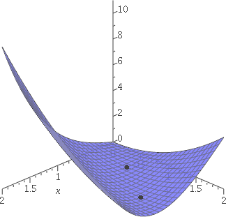
A picture might help. To the right is a graph of V when 0≤x≤2
and 0≤y≤2 made by Maple. The dots
( ) on the graph correspond to the values Euler
found. So when x=1 and y=3/2, V=1/4, and when x=1/2 and y=3/4,
V=5/16. Euler didn't have a computer but he was a human with
phenomenal ability to calculate. But this graph doesn't seem to show
any obvious behavior. ) on the graph correspond to the values Euler
found. So when x=1 and y=3/2, V=1/4, and when x=1/2 and y=3/4,
V=5/16. Euler didn't have a computer but he was a human with
phenomenal ability to calculate. But this graph doesn't seem to show
any obvious behavior.
|  |
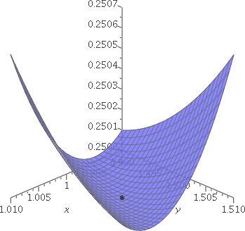
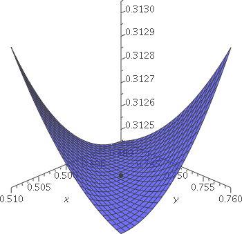
Below are "closeups" of the graph of V near the points (1,3/2,1/4) and
(1/2,3/4,5/16). These are graphs for x and y within .01 of the
identified values. These small local pieces of the graph don't
clearly show the type of the critical point. Certainly, neither of
them is a local max, but they could be saddles or local mins.
 |
 |
Graph of V for (x,y) near (1,3/2):
1–.01≤x≤1+.01;
(3/2)–.01≤y≤(3/2)+.01 |
Graph of V for (x,y) near (1/2,3/4):
(1/2)–.01≤x≤(1/2)+.01;
(3/4)–.01≤y≤(3/4)+.01 |
Algebraic analysis of Euler's function V with Maple
So here is the beginning. We declare V, compute first derivatives, and
find the critical points.
> V:=x^3+y^2-3*x*y+(3/2)*x;
                               3    2
                         V := x  + y  - 3 x y + 3/2 x

> Vx:=diff(V,x);Vy:=diff(V,y);
                                     2
                            Vx := 3 x  - 3 y + 3/2

                                Vy := 2 y - 3 x

> cps:=solve({Vx,Vy});
                  cps := {x = 1/2, y = 3/4}, {x = 1, y = 3/2}
Euler was correct. The two points he found are all of the critical
points of V. Declaring cps as the output of solve will allow us to use
the critical points later easily.
Now for the Second Derivative Test:
> Vxx:=diff(Vx,x);Vxy:=diff(Vx,y);Vyx:=diff(Vy,x);Vyy:=diff(Vy,y);
                                  Vxx := 6 x

                                   Vxy := -3

                                   Vyx := -3

                                   Vyy := 2

> H:=Vxx*Vyy-Vxy*Vyx;
                                 H := 12 x - 9

> subs(cps[1],[Vxx,H]);
                                    [3, -3]

> subs(cps[2],[Vxx,H]);
                                    [6, 3]
We find the second partial derivatives. Note that (of course!)
Vxy=Vyx. This use of Clairaut's Theorem is a
cheap way to check some of the computation. The H defined there is
usually called the Hessian (in the text, this is the
discriminant). The substitution commands
then compute both Vxx and H for each of the critical
points. Since H<0 at cps[1], which is (1/2,3/4), we learn that this
critical point is a saddle. At cps[2], which is (1,3/2), H>0 and
Vxx>0, so this critical point is indeed a local minimum.
The nature of critical points, even in dimension 2, can be
complicated! A great mathematician like Euler made mistakes.
The Gaussian bump
The function V invented by Euler is a typical textbook example. Over
the last few centuries, most of the examples appearing in textbooks
were quite tame: the critical points can be found by hand with some
algebraic effort, and then they can be classified with more
computation. Reality is rarely that straightforward.
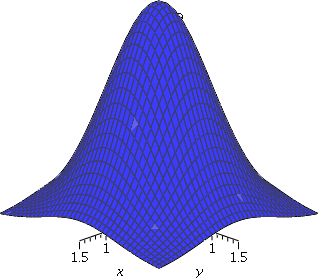
We consider f(x,y)=e−x2−y2. This
function is sometimes called a two-dimensional
Gaussian function. It is important in statistics, and in many
engineering and technical applications. A graph of f(x,y) for x and y
both in [−1.5,1.5] is to the right. Because we're dealing with an
exponential function, the values of f(x,y) are always
positive. Because −x2−y2 is always ≤0, the
values of f(x,y) are at most 1, so that 0<f(x,y)≤1. Of course,
f(x,y)=1 exactly when −x2−y2=0 which only
happens at (0,0). This is truly a bump of height 1, which has exactly
one critical point, a local and absolute maximum, at (0,0). Here is
Maple's confirmation, first discovering
the critical point.
> f:=exp(-x^2-y^2);
                                         2    2
                              f := exp(-x  - y )

> fx:=diff(f,x);fy:=diff(f,y);
                                            2    2
                           fx := -2 x exp(-x  - y )

                                            2    2
                           fy := -2 y exp(-x  - y )

> solve({fx,fy});
                                {x = 0, y = 0}

> cp:=solve({fx,fy});
                             cp := {x = 0, y = 0}
|  |
Now classification of this one critical point:
> H:=diff(f,x,x)*diff(f,y,y)-diff(f,x,y)^2;
                             2                 2           2  2   2
            H := (-2 %1 + 4 x  %1) (-2 %1 + 4 y  %1) - 16 x  y  %1

                                          2    2
                              %1 := exp(-x  - y )

> subs(cp,[diff(f,x,x),H]);
                                                2
                            [-2 exp(0), 4 exp(0) ]
Since e0=1, the Hessian is positive and the second partial
derivative with respect to x (twice) is negative. Therefore (0,0) is a
local maximum.
A more complicated example
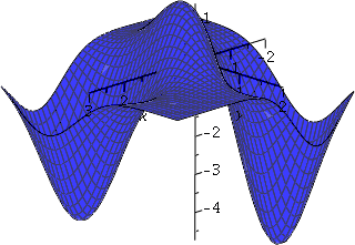 Here is a function F that's a linear combination of three bumps; a
bump of height 2 at (0,0), a bump of height −4 at (2,−1), and a bump
of height −5 at (−1,1):
F=2e-x2-y2-4e-(x-2)2-(y+1)2-5e-(x+1)2-(y-1)2.
A graph of F for x in [−2,3] and y in [−2,2] is shown to the right. It
is a complicated object. We should expect that the bumps interfere
with each other, but that the resulting graph will have a local max
near (0,0), and local minima near (2,−1) and
(−1,1). More precise location of these points might be useful in
applications. Also, are there other critical points? Where are they, and
what kind of critical points are they?
The last two questions might seem to be simple but they are not. A
series of detailed investigations of linear combinations of
only three Gaussians shows that the resulting function can have
from 1 to 7 distinct critical points. Answers to the questions are not
obvious!
Let's begin by trying to locate the critical points of F.
> F := 2*exp(-x^2-y^2)-4*exp(-(x-2)^2-(y+1)^2)-5*exp(-(x+1)^2-(y-1)^2);
             2    2                  2          2
F := 2 exp(-x  - y ) - 4 exp(-(x - 2)  - (y + 1) )

                     2          2
     - 5 exp(-(x + 1)  - (y - 1) )

> Fx:=diff(F,x);
                 2    2                             2          2
Fx := -4 x exp(-x  - y ) - 4 (-2 x + 4) exp(-(x - 2)  - (y + 1) )

                                2          2
     - 5 (-2 x - 2) exp(-(x + 1)  - (y - 1) )

> Fy:=diff(F,y);
                 2    2                             2          2
Fy := -4 y exp(-x  - y ) - 4 (-2 y - 2) exp(-(x - 2)  - (y + 1) )

                                2          2
     - 5 (-2 y + 2) exp(-(x + 1)  - (y - 1) )

> solve({Fx,Fy});
Warning, solutions may have been lost
> fsolve({Fx,Fy});
memory used=45.9MB, alloc=35.9MB, time=0.69
                   2    2                             2          2
fsolve({-4 x exp(-x  - y ) - 4 (-2 x + 4) exp(-(x - 2)  - (y + 1) )

                                2          2              2    2
     - 5 (-2 x - 2) exp(-(x + 1)  - (y - 1) ), -4 y exp(-x  - y )

                                2          2
     - 4 (-2 y - 2) exp(-(x - 2)  - (y + 1) )

                                2          2
     - 5 (-2 y + 2) exp(-(x + 1)  - (y - 1) )}, {x, y})
Both solve and fsolve give no information. The first response
("solutions may have been lost") says that solve ran into difficulties. The second response
is an echo of the command, so fsolve
can't go further.
About solve and fsolve
Generally, systems of several non-linear equations in more than one
variable can't be efficiently solved, and even numerical approximation
of solutions can be difficult. Lots of smart people have contributed
to Maple and tried to find solutions of
equations. Here is the official description of solve:
| |
The solve command solves
one or more equations or inequalities for their unknowns.
|
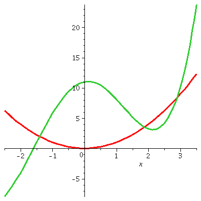
Even if only one equation of one variable is given, the solve command may not give a useful response.
For example, consider the equation
x2=10cos(x)+ex. To the right is a graph of the parabola, x2, and the more complicated cosine/exponential
function. The graph is correct, and the equation has three
solutions. However:
> solve(x^2=10*cos(x)+exp(x));
                                            2
                     RootOf(-10 cos(_Z) + _Z  - exp(_Z))
So solve doesn't help, except to signal
that Maple knows no simple way to
express the (possible!) solutions of the equation.
The command fsolve is used to
approximate solutions to equations. Its description states
| | The fsolve
command numerically solves one or more equations for their unknowns.
|
So we try it:
> fsolve(x^2=10*cos(x)+exp(x));
                                 1.876457458
If you check the graph, this is an approximate value for one root of
the equation. We can find the others. fsolve is a complicated collection of numerical
equation solvers. Perhaps think of it as a sophisticated
implementation of Newton's method, and any experience with such
algorithms suggests that success may depend on supplying a good
initial guess. We can consider the graph just shown, and try some
initial guesses.
> fsolve(x^2=10*cos(x)+exp(x),x=-1);
                                 -1.398935473

> fsolve(x^2=10*cos(x)+exp(x),x=2);
                                 1.876457458

> fsolve(x^2=10*cos(x)+exp(x),x=3);
                                 2.894494354
We get good approximations to all three of the roots the graph
suggests. Newton's method is sensitive to the initial guess, and
strange behavior can occur. Here, for example, an initial guess of 200
leads to the approximate root 2.894494354 but the guess −200 leads to
1.876457458, "skipping" the closer approximate root at −1.398935473.
Back to the critical points of F
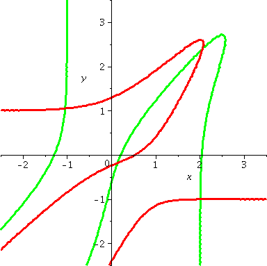 We'll use a picture to suggest good initial guesses for critical
points. Since a critical point solves the two equations
∂F/∂x=0 and ∂F/∂y=0, one way to get these guesses
is to consider a graph similar to what's shown here. It was created
with the following commands.
> intx:=-2.5..3.5: inty:=-2.5..3.5:
> A:=implicitplot(Fx=0,x=intx,y=inty,color=green,thickness=3,grid=[40,40]);
> B:=implicitplot(Fy=0,x=intx,y=inty,color=red,thickness=3,grid=[40,40]);
> display({A,B});
The grid option asks that the equation
Fx=0 be "sampled" at 40×40 points
in the specified rectangle. The default value of this parameter is
[26,26] which shows somewhat wiggly curves. But the curves really are
smooth. The slightly denser sampling creates a nicer picture that's
also more realistic. There is a cost because more function evaluations
must be done.
|
Important The graph shown has x and y between −2.5 and
3.5. This rectangle was used after some experiments suggested that the
critical points for this function were captured inside
it. The same rectangle won't necessarily be appropriate for other
functions! In general, you may need to consider several candidates for
reasonable rectangles. |
Now to get one critical point. If we look at the graph, one
intersection of the red and green curves is near the origin, (0,0).
> cp1:=fsolve({Fx,Fy},{x=0,y=0});
                 cp1 := {x = 0.1394363711, y = -0.1824419567}

> H:=diff(Fx,x)*diff(Fy,y)-diff(Fx,y)^2:

> evalf(subs(cp1,[H,diff(Fx,x)]));
                         [22.25153747, -5.485852297]
The use of : after the definition of the
Hessian means that the result is not shown. H has a long,
complicated formula and the details are not useful here. evalf prevents the appearance of many unsimplified
numerical expressions involving the exponential function. We're just
interested in the signs, in any case. So this critical point, with
positive Hessian and negative ∂2F/∂x2,
must be a local maximum. This agrees with the original graph of
F.
The coordinates for the red/green
intersections can either be guessed "by eye" or the cursor, with a
left click, can be moved to the desired point on the graph, and
coordinates read from the top of the Maple window.
> cp2:=fsolve({Fx,Fy},{x=2,y=-1});
                  cp2 := {x = 2.006534618, y = -1.003265964}

> evalf(subs(cp2,[H,diff(Fx,x)]));
                          [65.65902339, 8.182478048]

> cp3:=fsolve({Fx,Fy},{x=-1,y=1});
                  cp3 := {x = -1.046965891, y = 1.046967075}

> evalf(subs(cp3,[H,diff(Fx,x)]));
                          [108.2120134, 10.44438867]

> cp4:=fsolve({Fx,Fy},{x=2,y=2.5});
                  cp4 := {x = 2.071244361, y = 2.408645664}

> evalf(subs(cp4,[H,diff(Fx,x)]));
                                     -6
                    [-0.3399465012 10  , -0.000639824406]
So we have two local minima (near the centers of two of the
original unperturbed Gaussians) and one saddle point. The saddle is
quite flat because the Hessian has small absolute value (that's not an
obvious implication).
Maintained by
greenfie@math.rutgers.edu and last modified 7/14/2010.
 ) on the graph correspond to the values Euler
found. So when x=1 and y=3/2, V=1/4, and when x=1/2 and y=3/4,
V=5/16. Euler didn't have a computer but he was a human with
phenomenal ability to calculate. But this graph doesn't seem to show
any obvious behavior.


 Here is a function F that's a linear combination of three bumps; a
bump of height 2 at (0,0), a bump of height −4 at (2,−1), and a bump
of height −5 at (−1,1):
 We'll use a picture to suggest good initial guesses for critical
points. Since a critical point solves the two equations
∂F/∂x=0 and ∂F/∂y=0, one way to get these guesses
is to consider a graph similar to what's shown here. It was created
with the following commands.