A dynamic example of the argument principle
The Argument Principle deals with the behavior of simple closed curves
under "mappings" by functions f(z) which are analytic and not
zero on the closed curve, but which may have zeros and poles
inside the simple closed curve. The tool for investigating this is the
integral over the curve of the function f´(z)/f(z), the "logarithmic
derivative" of f(z).
Suppose C is such a closed curve, and f(z) is such a function. Inside
C, the function f´(z)/f(z) has isolated singularities at each
pole and each zero. The type of those isolated singularities of
f´(z)/f(z) at each of those points turns out to be just a simple
pole, that is, a pole of order 1. The residue at each point is +(the order of the zero) and -(the order of the pole). The Argument Principle
applies the Residue Theorem to the integral over C of f´(z)/f(z)
and then further analyzes the integral over C of that function. It
declares that the integral is the amount that the argument of f(z)
would change (increase or decrease) as z moves along C. The reason
this is true is that many different logs (as antiderivatives of
f´(z)/f(z), the integrand) can be used to "evaluate" the integral
along C.
An example
 Suppose f(z) is the function :
 [(z+1)3(z-i)2]
----------------
 [(z+3)3(z-1)1].
This function has zeros of order 3 at -1 and order 2 at i. It has
poles of order 3 at -3 and 1 at 1. So
- The Laurent series of f´(z)/f(z) centered at -1 in a disc
centered at -1 begins with the term 3/(z+3)+higher order terms (powers
of z+3).
- The Laurent series of f´(z)/f(z) centered at i in a disc
centered at i begins with the term 2/(z-i)+higher order terms (powers
of z-i).
- The Laurent series of f´(z)/f(z) centered at -3 in a disc
centered at -3 begins with the term 3/(z+3)+higher order terms (powers
of z+2).
- The Laurent series of f´(z)/f(z) centered at 1 in a disc
centered at 1 begins with the term 1/(z-1)+higher order terms.
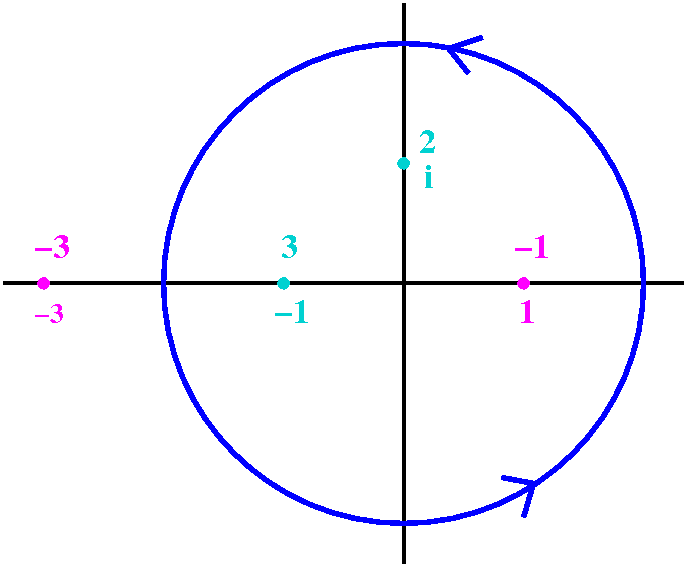
A sort of picture of these points is shown to the right. Now I want to
investigate what happens to the following simple closed curve:
s(t)=2eiπt with t in the interval [0,2Pi]. This is, of
course, a circle with radius 2 and center 0. So the circle encloses
three of the four points that are shown. The count should be
-1+2+3=4, and this, multiplied by 2πi, should be the increase in
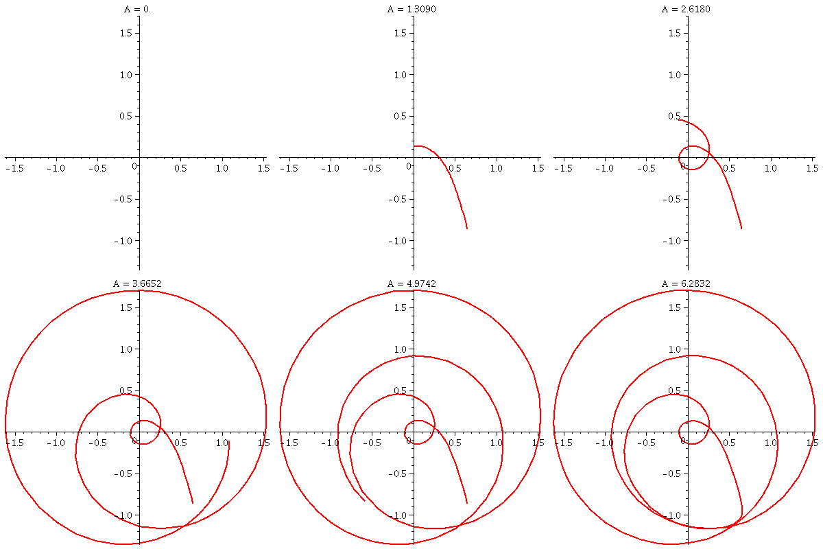
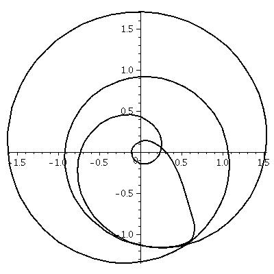
the argument of f(z) around C. The image curve in the complex plane is
shown in an animation created using Maple. If you are not using a fast connection,
then I apologize. The file size is half a megabyte! The picture on the
right is a still picture of the image of the circle. That may be
easier for people to see and study. I know as I try to count and see
how much the curve winds around 0, I almost got dizzy!
Do you believe the theorem? I will admit
that getting a nice-looking example took some experimentation. A great
deal of fussing was needed to see the loops. With a really "random"
example, the loops are all different scales, some large, some small.
Maintained by
greenfie@math.rutgers.edu and last modified 4/22/2008.
 Suppose f(z) is the function :
 Suppose f(z) is the function :