For this of course I needed to discuss simply connected: no holes, or the inside of any closed curve in the domain is also entirely in the domain. See pp.107-8 in the text.

I used the complex version of Green's Theorem for this result. See p.107 of the text. I remarked that the assumption of continuity for the derivative is not necessary. This is verified by Goursat's proof (see section 2.3.1) which is witty but will not be discussed by me, because I can't really see another use of the proof technique.

Then I went through the proofs of important theorems (see pp.107-111), including the Cauchy integral formula. I will continue with some of section 2.4 next time.

On Thursday
I will lecture from 6:10 to 7:10, take a 10 minute break, and then lecture for another hour. I would like to do this for the next few Thursdays and catch up with the other section.

HOMEWORK
Please hand in these problems on Thursday, March 24:
2.3: 1, 2, 4, 9, 10, 14.

Diary entry in progress! More to come.

The object of today's class is to again look at power series: SUM_n=0^infinitya_nzⁿ. Such series have a radius of convergence, R. Inside the radius of convergence, the series will converge to a sum, S(z), depending on z. This sum is a continuous function inside the radius of convergence. But more is true.

• If SUM_n=0^infinitya_nzⁿ has radius of convergence R, then SUM_n=0^infinitya_nnz^n-1 (the "term-wise" differentiated series) also has radius of convergence R.
• The function S(z) is complex differentiable, and inside the radius of convergence, S´(z)=SUM_n=0^infinitya_nnz^n-1.

THIS  IS  NOT  COMPLEX  ANALYSIS  SO  YOU  CAN  DISREGARD  IT! A Fourier series example Fourier series were basically introduced and used by Fourier in the 1820's to solve heat conduction problems. I handed out some pictures of Fourier series. I did not prove anything about these pictures, but I strongly suggested that they encouraged the belief that you can not always differentiate series of functions, term-by-term. Proving that the original Fourier series in these examples does converge to a continuous function is not difficult. Proving that the function is not differentiable and that the differentiated series does not generally converge would be much more difficut, and is something done in more advanced courses. But, please: the pictures should encourage you to be a bit careful.

I gave a good proof of the second fact above, that S(z) is differentiable, and that its derivative is the term-wise differentiated series. This is a technical proof, probably the most complicated to be done in the whole course. I did want to convince people that the result was true. The proof in the textbook actually is more-or-less the same, perhaps reordered in ways that I don't find so appealing. But basically you constantly compare to geometric series, you use the fact that [{S(z+h)-S(z)}/h]-S´(z) can be written nicely using the Binomial Theorem, and that the binomial coefficients are positive, so that things work well with the triangle inequality and rearrangement of series.

I did not give a proof or much of a discussion of the first claim, that the differentiated series had the same radius of convergence. The textbook's version is good, I think. Basically the assertion is that putting n in front of the terms of a power series doesn't much change how it converges (think of the ratio test!)

We can now apply our results again and again, to see that the sum of a power series can be differentiated as often as we want. And we can also see that if S(z)=SUM_n=0^infinitya_nzⁿ, then by repeatedly differentiating and letting z be 0, the coefficients a_n must be Sⁿ(0)/n!. So the power series is actually the Taylor series of its sum inside the radius of convergence.

Much more surprising things will occur!

• A chain rule computation from section 1.6 which leads to a neat result about evaluation of line integrals. I should have done this last time but I forgot.
• An example of pathology from the real calculus.
• Verification of the initial power series results, and discussion of some examples.

If I know that F(z) is analytic, and that F´(z)=f(z), and I have a curve C(t), for t in [a,b], then _Cf(z) dz=F(C(b))-F(C(a)). That is, the line integral of the derivative is the value at the END minus the value at the start.

So now we have another method to evaluate line integrals. Start with _C f(z) dz. IFwe know

• f(z) is the derivative of an analytic function, F(z).
• The domains of f(z) and F(z) include the curve, C.

For example, suppose f(z)=z⁵. This is an entire function, and I know it is the derivative of the entire function F(z)=[1/6]z⁶. Suppose C is any curve that starts from 2-i and ends at -1-i. Then _Cz⁵ dz=[1/6](2-i)⁶-[1/6](-1-i)⁶.

You should not suppose, though, that the restrictions about domain of f(z) and F(z) including C can be disregarded. We know that _unit circle(1/z) dz=2Pi i. Since if we did have an f(z)/F(z) pair where f(z)=1/z, the integral over a closed curve would be 0, we can conclude that there is no function analytic in a domain which includes the unit circle whose derivative in that domain is 1/z. "Locally" on pieces of the circle (in fact, any piece of the circle which discards one point) we can in fact find such an antiderivative. The function Log(z) is an antiderivative of 1/z, where we discard -1 from the circle.

THIS  IS  NOT  COMPLEX  ANALYSIS  SO  YOU  CAN  DISREGARD  IT! An example having little to do directly with this course, but it is an example which you should keep in mind because it will help you appreciate the special and rare beauty of the results of this course. Consider the real function of a real variable defined in a piecewise fashion by { exp(-1/x) for x>0 f(x)= { { 0 for x<=0. To the right is a Maple graph of this function. On the left, of course we have a half line. Since the real exponential function of negative reals is between 0 and 1, the graph on the right must be between y=0 and y=1 (if x>0 it can't equal 0 since the exponential function is never 0, and it can't equal 1 because 1/x can never be 0). Of course, on the left all of the derivatives are 0. What about on the right, where x>0? There f´(x)=e-1/x[1/x2]. Since this is always positive, we know that f increases. In fact, the right-hand limit at 0 of e-1/x "is" enegative infinity so it is 0. The function is continuous at 0, and therefore continuous everywhere. As x-->infinity, e-1/x-->e0=1. The Maple graph is totally justified. I would like to investigate finer properties of the function f(x). In particular, I would like to look at its differentiability at 0. The left-hand derivative of f(x) at 0 certainly exists and is 0. What about the right-hand derivative? For x>0, [{f(x)-f(0)}/{x-0}] is the same as (1/x)e-1/x. What happens as x-->0+ to this? Well, this is a Calc 2 exercise in L'Hopital's rule. I guess I would do it this way: As x-->0+, then w=1/x-->+infinity. And (1/x)e-1/x becomes w e-w=[w/ew]. This satisfies the criteria for L'H, so its limit is the same as the limit (if it exists) of [1/ew] as w-->+infinity. That's certainly 0. In fact, as I hope most of you remember, exponential growth is much faster than any polynomial growth. I now know that f(x) is differentiable, and that its derivative is { (1/x2)exp(-1/x) for x>0 f´(x)= { { 0 for x<=0. Let me do one more step. f´´(x) must exist away from 0 (I can use the product and Chain Rules on the right). What about f´´(0)? From the left again we see that the appropriate limit is 0. From the right, we officially need to consider [{f´(x)-f´(0)}/{x-0}] as x-->0+. Let's insert the formula for f´(x) and the value (just 0) of f´(0), so that we see we need to consider (1/x3)exp(-1/x) as x-->0+. But (w=1/x) this is w3/ew as w-->infinity, and the limit is 0. An official proof needs induction, etc., but I don't need no steenkin' official proof ... In fact, this function f(x) is infinitely flat at the origin. It and all of its derivatives exist at 0, and the values of the function and all of its derivatives at 0 are 0. Suppose we wanted a power series which would equal f(x), a power series centered at 0. Well, if the series work the way they should (and they do) then the power series will be a Taylor series for f(x) at 0. But all of the coefficients will be 0. So here's a function which can't be equal to a power series in any interval centered at 0, even though we can differentiate the function as much as we want. Nothing that bad occurs in complex analysis.

Elementary theory of power series
A power series centered at z₀ is a sum of the form SUM_n=0^infinitya_n(z-z₀ⁿ where all of the a_n's are complex numbers. Most of the time I will write power series centered at z₀=0 because I am lazy. We say that the power series converges if the sequence of partial sums has a limit. If the power series converges absolutely (that is, the series SUM_n=0^infinity|a_n| |z|ⁿ, a sequence of non-negative numbers) then the series will converge. I discussed this in lecture #4.

Radius of convergence
Suppose SUM_n=0^infinitya_nzⁿ converges for some non-zero z (any power series will always converge at its center, here when z=0). Then the pieces of the series can't get large: that is, the max of |a_n| |z|ⁿ is finite (or else the successive partial sums, which should converge, will take bigger and bigger "steps" from each other. Suppose this max is some number V. Look at what happens if we take a complex number w with |w|<|z|. Then |SUM_n=0^infinitya_nwⁿ|<=SUM_n=0^infinity|a_n| |w|ⁿ<SUM_n=0^infinity|a_n| |z|ⁿ[|w|/|z|]ⁿ. Now look closely.
|w|/|z| is some number r with r<1. We concluded that the other "stuff", |a_n| |z|ⁿ, is bounded by some big number, V. So therefore we are left with the overestimate, SUM_n=0^infinityV rⁿ with r a positive real number which is less than 1. But this series converges. So the original series, SUM_n=0^infinitya_nwⁿ, converges absolutely, and therefore converges.

Now we need to think about the situation a bit. As soon as you know the power series converges at a complex number, the series will converge absolutely at any complex number closer to its center. So the situation is like this: either the series converges for all complex numbers (perfectly possible, consider SUM_n=0^infinity[zⁿ/n!]) or it converges for no complex number except for the center (perfectly possible, consider SUM_n=0^infinityn! zⁿ]) or there are some complex numbers for which it diverges and some for which it converges. But then the computation we just made shows that if we consider the modulus of every complex number for which the series converges, then a circle (centered at the center of the power series) of such modulus must have all convergent numbers in it. Take the union of all those circles. The result will be a circle, and its radius is the radius of convergence.

Continuity of the sum
Look at SUM_n=0^infinitya_nzⁿ and suppose it has radius of convergence R>0. Here "infinity" is a possibility and infinity will be >0. Let's call the sum of this series, S(z). If |z|<R, the series converges absolutely. Fix some z inside the circle of convergence. Take some number r>0 so that |z|+r is still less than R (possible -- you could take r=(1/2)[R-|z|], for example). Then SUM_n=0^infinitya_n(z+w)ⁿ will converge absolutely for all w's with |w|<r. Not only that, but if we compare "infinite tails" of series, we also know that SUM_n=N^infinity|a_n| |z+w|ⁿ<SUM_n=N^infinity|a_n|(|z|+r|)ⁿ. Since the series SUM_n=0^infinity|a_n|(|z|+r|)ⁿ converges, I can choose N so that the tail, SUM_n=N^infinity|a_n|(|z|+r|)ⁿ is less than epsilon. But then look at what we have left out: SUM_n=0^N-1a_n(z+w)ⁿ. This is a polynomial. If w-->0 this polynomial will eventually differ by epsilon from its value at z, because polynomials are continuous.

Hey, I've just shown you that by neglecting an appropriate infinite tail, you can make the terms of a power series vary continuously. That means that the sum of the series, S(z), will be a continuous function inside its radius of convergence. This is dandy.

We reviewed and tried to understand what differentiability means
What's complex differentiability? Well, we want the limit

      f(z+h)-f(z)
 lim -------------
h-->0      h

 f(z+h)-f(z)
------------- = f´(z)+Err(f,z,h)
      h

f(z+h)=f(z)+f´(z)h+Err(f,z,h)h

Compatibility conditions
I remarked that linear algebra tries to study collections of linear equations systematically (a little math joke in that phrase, sorry). So maybe one studies M equations in N unknowns. There are only a few rather rough things one can learn in general. For example,
a homogeneous system of M equations in N unknowns with more unknowns than equations (N>M) must always have non-trivial (non-zero) solutions.
And here's another:
If you have more equations than unknowns (M>N), in general the equations can't be solved: they don't have solutions unless certain additional conditions ("compatibility conditions") are satisfied.

For example,

2x+3y=A
 x+2y=B
5x+4y=C

And now back to complex analysis ...
Last time we tried to solve

vx=-2y
vy=4x3

Fact from calc 3 If a function has is continuous second partial derivatives, then its mixed second partial derivatives must be equal. The proof uses the Mean Value Theorem.

So look at the Cauchy-Riemann equations:
   u_x=v_y
   u_y=-v_x
Differentiate the first with respect to x and the second with respect to y. We get
   u_xx=v_yx
   u_yy=-v_xy
Since v_yx=v_xy I know that u_xx=-u_yy, usually written
   u_xx+u_yy=0
This is Laplace's equation, and the stuff on the left-hand side is called the Laplacian of u. Solutions of Laplace's equation are called harmonic functions, and harmonic functions come up all over the place. Notice, please, that x⁴+y² is not harmonic, so it cannot be the real part of a complex differentiable function.

Harmonic; conjugate harmonic
In fact, if f(z) is complex differentiable, with f(z)=u(x,y)+iv(x,y), then both u(x,y) and v(x,y) are harmonic functions. v(x,y) is called a harmonic conjugate of u(x,y). It is interesting to realize that a "random" polynomial in x and y is very unlikely to be harmonic. In fact, a goal of the course is to justify interest in these rather rare (?) objects.

The converse to CR
Suppose that u(x,y) and v(x,y) have continuous first partial derivatives. Further suppose that the Cauchy-Riemann equations are correct at a point (x,y):
   u_x=v_y
   u_y=-v_x
Then f(z)=u(x,y)+iv(x,y) is complex differentiable at z=x+iy.

I actually attempted to verify this. I know another fact from calc 3. I h=a+ib (think of a and b as very small):
u(x+a,y+b)=u(x,y)+u_x(x,y)a+u_y(x,y)b+Err₁(u,x,y,a,b)(|a|+|b|)
v(x+a,y+b)=v(x,y)+v_x(x,y)a+v_y(x,y)b+Err₂(v,x,y,a,b)(|a|+|b|)
and Err₁(u,x,y,a,b) and Err₂(v,x,y,a,b) both -->0 as a and b both -->0. Now let's look at f(z+h)=u(x+a,y+b)+iv(x+a,y+b). This is
[u(x,y)+u_x(x,y)a+u_y(x,y)b+Err₁(u,x,y,a,b)(|a|+|b|)]+i[v(x,y)+v_x(x,y)a+v_y(x,y)b+Err₂(v,x,y,a,b)(|a|+|b|)]
Let us reorganize this stuff:
u(x,y)+iv(x,y) (this is f(z))
{u_x(x,y)a+u_y(x,y)b}+i{v_x(x,y)a+v_y(x,y)b}
Now if A=u_x=v_y and B=u_y=-v_x, this becomes
{Aa+Bb}+i{-Ba+Ab} and we can recognize this as (A-iB)·(a+ib). If we think about this, then f´(z) should be A-iB and a+ib is h, so we have f´(z)h.

What's left over? This:
{Err₁(u,x,y,a,b)(|a|+|b|)}+i{Err₂(v,x,y,a,b)(|a|+|b|)}
I would like this to be Err(f,z,h)h. Remember that all the Err terms go to 0 as a+ib-->0. What's left to consider? Well, |h|=sqrt(a²+b²) compared to |a|+|b|. So I'll compare them.

Inequalities
Surely sqrt(a²+b²)<=|a|+|b| because if you square both sides, you get a²+b²<=|a|²+2|a| |b|+|b|². Now cancel a² with |a|² and b² with |b|² and we get 0<=2|a| |b| which is certainly true.

Since sqrt(a²+b²)<=|a|+|b|, I know that if |a|+|b|-->0, then |a+ib|-->0. What about the converse?

Look at |a|+|b|<=2sqrt(a²+b²). I think I tried 2 in class. Now square and see if we can clarify things:
|a|²+2|a| |b|+|b|²<=4(a²+b²). We can cancel some terms, and get
2|a| |b|<=3(a²+b²).
But 2|a| |b|<=a²+b² is true, because 0<=a²-2|a| |b|+b²=(|a|-|b|)² is certainly true.

Since |a|+|b|<=2sqrt(a²+b²) I now know that if |h|=|a+ib|-->0, then |a|+|b|-->0. Wow! We are done.

What about |z|²?
If f(z)=|z|²=x²+y², at which points is f(z) complex differentiable? I just need to check the Cauchy-Riemann equations when u(x,y)=x²+y² and v(x,y)=0. Then:
   u_x=v_y becomes 2x=0.
   u_y=-v_x becomes 2y=0.
So |z|² is complex differentiable only at the point z=0.

More vocabulary: analyticity (holomorphicity?)
It turns out that complex differentiability is not quite the correct definition. Here's the correct definition:
A function f(z) defined on a connected open set is (complex) analytic if f(z) is complex differentiable at every point of the set.
This definition allows a neat theory. I remark that the word holomorphic is used instead of analytic sometimes.

f´=0
Here's a first fact: if f(z) is analytic and if f´(z)=0 for all z, then f(z) is constant.

Notice that if the domain of f(z) is not a connected open set, then this result is false, because you could have f(z) equal to one constant in one "blob" and another constant in another "blob".

Well, if f´(z)=0 for all z, then then Cauchy-Riemann equations, combined with the observation that f´(z)=u_x+iv_x show that u_x=0 and u_y=0 and v_x=0 and v_y=0 for all x and y. This means that u and v must be constant on horizontal lines (because of the x derivatives) and on vertical lines (because of the y derivatives). But in a connected open set, any two points can be connected, not only by line segments, but also by line segments which are made up entirely of horizontal and vertical line segments. So the values at any two points must be equal because of the previous observations about vertical and horizontal lines.

Other conditions
If f(z) is analytic and has only real values, then f(z) is constant.
Why? Because then v is 0, and so v_x=0 always and v_y=0 always, then the Cauchy-Riemann equations tell you that f´(z) is 0 always. So f(z) must be constant.

If f(z) is analytic and has only imaginary values, then f(z) is constant.
Why? Interchange u and v in what we just did.

If f(z)=u(x,y)+iv(x,y) where u and v are real, and if u²+v² is constant, then f(z) is constant.
Look at the clever proof on p.82 of the text. Here is another proof, not so clever: if u²+v²=C, then d/dx this equation. The result is
   2u u_x+2v v_x=0.
Of course we can do the same thing with d/dy:
   2u u_y+2v v_y=0.
Now use the Cauchy-Riemann equations. This will get us:
   2u u_x-2v u_y=0.
   2u u_y+2v u_x=0.
Look closely at this system of equations:

(2u -2v)  ( ux )   (0)
(      )  (    ) = ( )
(2v  2u)   (0)

Why? Geometry for the future
The previous results are actually reflections of the following truth: if an analytic function is not a constant function, then the image of the domain of the analytic function will always be an open subset of C. This is not obvious, and nothing like it is true in elementary real analysis.

Exam warning!
I'll give an exam a week from Tuesday. The exam day is therefore Tuesday, March 1.

HOMEWORK
Please begin to read section 2.2 (sorry, Mr. Cohen, I am skipping 2.1.1).
2.1: 23
In class I exhibited a function which was complex differentiable only at 0. Can you find a function defined on all of C which is complex differentiable only at 0 and 1?
2.2: 2, 3, 9, 11, 13, 14, 17

HOMEWORK
Please begin reading Chapter 2, and do the previously assigned problems. Some of them are difficult.

• Mardi Gras!
• The Chinese New Year, the year of the Rooster!!
• Valentine's Day!!!

Cu(z) dz      Here are some facts we need to know about line integrals.

The definition

In this course, line integrals will be defined for piecewise differentiable parameterized curves, C, and for u(z)'s which are continuous on the curve's image. I noted that it is possible to define the integrals using a sort of Riemann sum procedure, by sampling the function u(z) along the curve and multiplying by the lengths of the edges of a corresponding polygonal approximation to the curve. Then we would take the limit as the mesh (the length of the longest side in the polygon) goes to 0. Then, using the Mean Value Theorem, we'd get the same result for our collection of curves. Also, line integrals frequently are associated with actual physical quantities such as work, flux, etc. These quantities are most easily recognized using the Riemann sum definition.

Independence of parameterization

One consequence of our definition of line integral is that we should prove or verify that value of the line integral does not depend upon parameterization. I gave an example last time which showed this. That is very different from proving that equality holds in all cases, as I hope you realize.

Linearity in the integrand, u(z).

If k is a constant, and u₁ and u₂ are eligible integrands, then _Cku₁(z)+u₂(z) dz=k_Cu₁(z) dz+_Cu₂(z) dz.
This certainly looks o.k.: it looks like something we've been accustomed to for years.

"Linearity" (as much as you'll let me!) in the curve, C.

What the heck does this mean? Well, for one thing, when we can add curves, the corresponding integrals add. So if C₁ and C₂ are curves with the correct HEAD/TAIL relationship, then _C1+C2u(z) dz=_C1u(z) dz+_C2u(z) dz.
Reversals work nicely, also: _-Cu(z) dz=-_Cu(z) dz.
These things are very convenient in practice, and I will probably use them (I did later in class!) without even a proper citation. They are just so familar and neat -- after they have been learned!
People have extended "linearity in C" in various ways whenever it has been useful. We may need some of this later.

Estimating the integral, with weak and strong justification.

Let me begin with an example, which I should have done in class. I need to choose the darn example very carefully, to have a hope of computing it "by hand".

Let's compute ₀¹t²+2ti dt. (Why do I need to be so careful? Wait, wait.) I can antidifferentiate polynomials. This works out to (1/3)+i. The modulus of this complex number answer is sqrt(10)/3, which is about 1.054092553. Therefore the modulus of the integral is about 1.054092553.

Much of mathematics is not very subtle. A great deal consists of trying to find out if changing the order of doing things changes the answer. Here the "things" are integration and taking modulus. Onward!

The integrand is t²+2ti, and its modulus is sqrt(t⁴+4t²) which is t sqrt(t²+4). Hah! The alert Calc 1 student will now see that this is a function whose antiderivative can be easily written: it is (1/3)[t²+4]^3/2. So I can compute the integral of the modulus of this function exactly, and the answer is (5/3)sqrt(5)-(8/3), A numerical approximation of this is 1.060113297.

These computations have been facilitated by my friend, Maple.

What have I done? I have computed ₀¹|g(t)| dt and |₀¹g(t) dt|. The first is approximately 1.060113297 and the second is approximately 1.054092553.

Now let me give you a heuristic reason for a more general assertion. Of course, heuristic means

adj. 
1. allowing or assisting to discover.
2. [Computing] proceeding to a solution by trial and error.

Suppose g(t) is a complex-valued function defined for t's in the interval [a,b]. Now _a^bg(t) dt is, to me, really a BIG (Riemann) sum: SUM_j=1^Ng(t_j)(t_j-t_j-1). How large can this be? Since the complex numbers can't be ordered, I use modulus instead, and ask how large can |SUM_j=1^Ng(t_j)(t_j-t_j-1)| be? The Triangle Inequality applies here, and an overestimate is SUM_j=1^N|g(t_j)|(t_j-t_j-1). I don't need the | | around (t_j-t_j-1) because (t_j-t_j-1) is a positive real number. But SUM_j=1^N|g(t_j)|(t_j-t_j-1) is a Riemann sum for another integral: _a^b|g(t)| dt. All of this leads me to believe that
|_a^bg(t) dt|<=_a^b|g(t)| dt.

This inequality is correct. We have seen one numerical agreement. The discussion using Riemann sums is quite difficult to convert into a proof. There is a very nice, rather tricky, device to prove this result on p.61 of the text, which you might want to look at.

The ML inequality

The previous result will be used a great deal in this course but it will be applied to line integrals. If z(t) is the parameterization for the curve C, when t is in the interval [a,b], and if z(t) is differentiable (both x(t) and y(t) are differentiable), then _Cu(z) dz=_t=a^t=bu(z(t))z´(t)dt. The inequality we just developed then states:
|_t=a^t=bu(z(t))z´(t)dt|<=|u(z(t))| |z´(t)| dt. The next step depends on clever recognition of a formula and knowing what the aim of the manipulation is. As I described in class, the aim is sort of a decoupling (as things are called in physics) or a disconnection between the curve, C, and the integrand, u(z). We will necessarily lose some precise information but in applications it will turn out that the estimates we can make are the important consequences. So consider: suppose that we know, from somewhere, that the function u(z) has some overestimate in modulus on the curve, C. That is, there is a non-negative real number M so that |u(z)|<=M for all z on C. Then |u(z(t))| |z´(t)| dt<=M |z´(t)| dt. But,hey!, |z´(t)| is sqrt[{x´(t)}²+{y´(t)}² and maybe you recognize the integral: it defines (or computes, depending on your choice of textbook!) the length of the curve. Whenever possible in this course, I will label the length of C with the letter L. So:
|_Cu(z) dz|<=ML.

This inequality will be used about 370 times by the instructor and by students in the course. Let me show you some examples, which will be silly because they are out of context.

ML example #1
I considered the curve S_R, which I drew on the board. It was a semicircle of radius R in the upper halfplane, centered at the origin. The integrand was 1/z². I wanted to investigate the asymptotics of _SRdz as R-->infinity. In this case the integral can be evaluated exactly, but I wanted ot use the ML inequality. So:
|_SRdz|<=ML. Here L is half the circumference of a circle of radius R, and that's (Pi)R. What about M? Well, on the curve, |z|=R. so |1/z²|=1/R². Therefore the modulus of the integral is at most (Pi)R(1/R²). The R² on the "bottom" dominates as R-->infinity, so certainly this integral must-->0.

ML example #2
I used the same S_R, but now I wanted a more interesting u(z). I think I tried something like u(z)=1/[z⁴+5z+4]. The exact numbers don't matter: what does matter is the estimation. Again, to understand the asymptotic behavior as R-->infinity, I used ML, and L was PiR as before. Since u(z) is a bit more complicated, I had to use the techniques introduced in Lecture #2 to estimate it. We did some examples then which you may review.

Suppose |z|>10 (mostly picked at random). Then |z⁴+5z+4|>=|z|⁴-|5z+4|. But how large can |5z+4| be? Well, on S_R where |z|=R>10, I know that |5z+4|<=5|z|+4<=2|z|². But 2<=(1/2)|z|² for these z's, and therefore |5z+4|<=(1/2)|z|⁴, and |z⁴+5z+4|>=|z|⁴-(1/2)|z|⁴=(1/2)|z|⁴. There is a great deal of sloppiness and waste in here: the inequalities are likely to be very far from equalities but I just want to get an answer.

Now I know for z on S_R, |u(z)|<=1/[(1/2)|z|⁴] so that I can take 2/R⁴ as my M. The modulus of the integral is therefore bounded by (Pi)R[2/R⁴] and this surely -->0 as R-->infinity. In this case, I don't it is at all possible to compute exact values of the integral, but the estimation is very easy.

Green's Theorem

So here is what it's about: line integrals over closed curves. I will compute a line integral over a closed curve. Indeed, the closed curve I will use will be the boundary of the unit square (both x and y in the interval [0,1]), and the integrand will be the innocent function, x. So let me compute _{Bdry square}x dz. I will compute it using four parameterizations and the whole integral will be the sum of four pieces. There are several reasonable ways to parameterize some of these pieces and some of these ways are different from those I choose.

	t is in [0,1] z=t x=Re(z)=t dz=dt 01t dt=1/2	t is in [0,1] z=it+1 dz=i dt x=Re(z)=1 01i dt=i/2	t is in [0,1] z=-t+1+i dz=-dt x=Re(z)=-t+1 01(-t+1) -dt=-1/2	t is in [0,1] z=i-it dz=-i dt x=Re(z)=0 010 i dt=0

Therefore the integral is 1/2+i/2-1/2+0=i/2. This isn't 0: what a disappointment. Sometimes people misremember Green's Theorem and it might sound like the line integral over almost any closed curve of almost anything is 0. That is far from true.

A sort of statement of Green's Theorem
Well, let me quote the result in the text:
_Gammaf(z) dz=i _Omega[f_x+if_y]/2 dxdy.
Here Gamma is the whole boundary curve of a region Omega, oriented so that the region is the left of the curve Gamma as we more along Gamma. This is a Green's Theorem changed so that we can use it in complex analysis. The f_x and f_y are the partial derivatives with respect to x and y. We can check it for the case we just computed. The double integral's integrand, [f_x+if_y]/2, is 1/2, and the area of the square is 1, and the i out in front makes everything come out correctly.

A sort of proof
If we wanted to check more generally (whisper the word, proof) then ... well, since both sides are linear we could start with looking at i _Omega[f_x]/2 dxdy. We can use the Fundamental Theorem of Calculus to convert the partial with respect to x into f(1,y)-f(0,y) because the integral over the unit square has both x and y going from 0 to 1. Then the double integral becomes i_y=0^y=1[f(1,y)-f(0,y)]/2 dy. This then breaks up (and I'll change y to t): _t=0^t=1f(1,t) i dt-_t=0^t=1f(0,t) i dt. The first of these integrals is the integral of f(z) over the right-hand side of the boundary of the unit square, going up, and the second is the integral of f(z) over the left-hand side of the unit square, going down. The other two sides are gotten from the f_y term in a similar manner.

Now look at the important integral ...
We previous computed the most important line integral. Let's try it again. Here f(z)=1/z=1/(x+iy), and the region, Omega, is the circle of radius R centered at the origin. The corresponding double integral has as integrand [f_x+if_y]/2. I'll use the Chain Rule and get f_x(z)=-[1/z²]1 and f_y(z)=-[1/z²]i. Therefore the integrand [f_x+if_y]/2= -[1/z²]1+i-[1/z²]i=0 if we recognize that i² is -1. So use of Green's Theorem in this most important example yields 0. This is distressing since we previously computed it and got 2(Pi)i. What is wrong? The use of Green's Theorem here is not valid.

Better state Green's Theorem more precisely
The functions in Green's Theorem need to be differentiable ("smooth") at every point on and inside the curve. Even one "lousy" point (a singularity) makes it possible for the theorem to be not correct. This is subtle, and you should reinforce it by thinking, again and again, that 2(Pi)i is not the same as 0.

Now look at what "inside" means using a weird computation
Let's try to compute _B(1/z) dz. Here B is the orinted boundary of the square whose sides are parallel to the coordinate axes, centered at 0, and whose side length is 4. A direct computation by parameterization of this integration is (barely) possible. I've done it and it is very tedious and very unpleasant. We can be, instead, a bit devious, and compute the integral quite easily.

As indicated in the picture, the curve A will be the positively orineted unit circle with center 0. The region R is the subset of C between these curves. Notice that the correctly oriented boundary of R is B-A. The minus sign is very necessary. We can apply Green's Theorem to this R with 1/z, because the only singularity, 0, is outside of R and A and B. But we saw that the integrand of the double integral for this function is 0 before (when we computed [f_x+if_y] for f(z)=1/z. Therefore the double integral term in Green's Theorem is 0. What's the other side? It is _B-A1/z dz. Thus _B-A1/z dz=0, or _B1/z dz-_A1/z dz=0 or _B1/z dz=_A1/z dz. But the A integral is 2(Pi)i, and therefore the B integral is 2(Pi)i. This is quite tricky, and I will essentially use ideas like this frequently in the remainder of the course.

What's inside?
The logic of the preceding computation can be generalized, so that if C is a closed curve (oriented positively) and p is a point not on C, the _C[1/(z-p)] dz is either 0 or 2(Pi)i. In the first case, p is outside of C and in the second case, p is inside C. Maybe this is how to figure out what inside and outside are!

HOMEWORK
Please begin to read Chapter 2 of the text.
Please hand in these problems on Thursday, February 17:
1.6: 7, 15
2.1: 1a, 6, 14, 16, 20c,e

The linkage experiment

The mechanism of the Mad Count

Here is an interesting and startling experiment which I tried in class. Imagine this story: a Mad Scientist, Count Ogus von Brandenburg of Bavaria, learned some complex analysis in 1830. He then devoted the remainder of his life and the resources of his principality to constructing mechanical devices which imitated complex mappings. In particular, he fell in love with the exponential mapping. He constructed a linkage which would allow a point in the range to be attached to several points in the domain, and the domain points would all be mapped to the given range point by the exponential mapping. A sort of drawing of part of the count's mechanism is shown above. I tried to simulate the mechanism of the crazy count in class.

Four of the wonderful students in the class volunteered (always better than the truth, which is closer to were dragooned) to draw some pictures with me. I only show the results of three of the students. I set up the exponential function mapping from a domain copy of C to a range copy of C. Then I stood at the range copy, with my chalk at w=1, which I also called HOME. I asked each of the students, each with their individually colored chalk, to choose a value of log(1). Since this is a complex analysis course, there were certainly enough distinct values to choose from. Each student could have their own value of log(1). In my head (sometimes small, sometimes large, frequently empty) I saw a sort of mechanical linkage reaching backwards from my 1 to their choices of log(1). The linkage would "automatically" respond to any changes of position in my location by moving to nearby places whose value of exp would be where my chalk moved to. Sigh. There's no pathology in this course: things will be continuous, things will move nicely, etc. Much more subtle problems will be met.

The first trip Then I carefully and slowly (well, almost) moved my chalk from HOME in a simple closed curve. The curve was made up of circular arcs centered at the origin and pieces of rays which started at the origin. I used these curves because last time we had previously computed how vertical and horizontal lines in the domain were mapped. The inverse images of my "trip" from HOME to HOME were carefully drawn. They were congruent, because exp is 2Pii periodic. Each started from each student's choice of log(1) and returned to that choice.

The second trip Well, now I left HOME and traveled in a circle around 0, and returned to HOME. The students attempted to imitate the Mad Count's device, and there was some controversy. If we tried to make everything continuous, then, even though my path in the range was a simple closed curve, each student draw a path going from one choice of log(1) to another choice of log(1). This is very, very mysterious. I drew a few more paths in the range and mentioned what would happen in the domain, and said we would need to explain all this is great detail later. This is one of my goals in the course.

Right now, no sine, no cosine!
Section 1.5 of the text discusses sine and cosine. I will save these functions until later. I want to get into the "core" of the course (and the subject) as soon as possible.

Vocabulary about curves
This stuff, which must be understood by 403 students, should have been covered in any calc 3 course, and is discussed in section 1.6 of the text.

Phrase	Proper definition	Possible picture
Curve	A curve is a function whose domain is an interval, [a,b], in R, and whose range is in C. If C(t) is the curve, we could write C(t)=x(t)+iy(t). In this course, these functions will generally be at least continuous.
Smooth (differentiable) curve	C(t)=x(t)+iy(t) should be differentiable, so that x(t) and y(t) are differentiable. Such a curve has a nice tangent vector at every point.
Piecewise smooth curve	The curve C(t) is certainly continuous. But additionally, we can divide the interval [a,b] into a finite number of pieces, and in each of these subintervals C(t) is smooth. This will allow us to take care of curves with finite numbers of corners, for example.
Simple curve	A simple curve is one which does not intersect itself except maybe ... at the ends (see the next plus one definition). So if the domain of C(t) is [a,b], and if a<s<t<b, then C(s) is not equal to C(t), and C(a) is not C(s) and C(b) is not C(s).
Closed curve	"Head=Tail" -- that is, if the domain of C(t) is {a,b], then C(a)=C(b).
Simple closed curve	A closed curve which is also simple. Here C(s)=C(t) with s<b implies either s=t or a=s and b=t.
Adding curves	Suppose C1(t) is a curve with domain [a,b] and C2(t) is a curve with domain [c,d]. If C1(b)=C2(c) (that is, C1's "Head"=C2's "Tail", perhaps) then the curve C(t) whose domain is [a,b+d-c] and defined by C(t)=C1(t) if t<b and C(t)=C2(t-b+c) (I hope!) is called the sum of C1 and C2. We will write C=C1+C2.
Reversing curves	If C(t) is a curve with domain [a,b], then the "reversal of C(t)", also called -C, will be the curve, let me temporarily call it D(t), whose domain will also be [a,b], defined by D(t)=C(b+a-t). -C is just C backwards. The picture is slightly weird (how should I have drawn it?) but I hope you get the idea.

I hope the darn formulas for C₁+C₂ and -C(t) are correct. I don't think I will ever be so formal again in this course. I will usually be rather casual. The curves in this course will all be piecewise differentiable, and, actually, they will turn out to be sums of line segments and circular arcs: HAH! to general theory!

Actually I should acknowledge that what we are defining are called parameterized curves. For example, the curves C(t)=t and C(t)=t² (use [0,1] as domains in both cases) are really different, even though they "look" the same. It turns out that we will mostly be interested in line integrals and a remark below about the values of the integrals explains why we will not care about different parameterizations.

A few examples

This curve is a straight line segment starting at -4i and going to -2i, followed by a quarter circle whose center seems to be 0, starting at -2i and going to 2. If I wanted to be totally strict, I guess I could define a C(t) on the interval from [0,2+(Pi/2)] Let's see: for t in [0,2), let C(t) be (t-4)i, and for i in [2,2+(Pi/2)], define C(t) to be 2ei(t-2-(Pi/2)). Some remarks Almost always in this course I will parameterize circles and circular arcs using the complex exponential. My first guess will always be CENTER+RADIUSei(stuff). Another remark: what I've just done is excessively precise and maybe slightly silly. I want to write curves in a way that is convenient. So this curve should be written as a sum of two curves, say C1+C2. Here C1(t)=ti where t is in the interval [-4Pi,-2Pi], and C2(t)0+2eit where t is in the interval [-Pi/2,0]. It is just easier to do this than to try to figure out the total length, how to combine and adjust parameterizations, etc.

Here I will write the curve again as a sum, C1+C2. C1 seems to be a semicircle of radius 2 and center -1. It goes backwards. So C1(t)=-1+2ei([Pi]-t) where t is in the interval [0,Pi]. C2 is a straight line segment. This I know how to parameterize from thinking about convexity. C2(t)=t(1)+(1-t)(-3i) where t is in the interval [0,1]. A remark Parameterizing a circular arc in a clockwise fashion feels close to obscene to me. Almost always in this course our circles will be parameterized positively, which will mean counterclockwise.

Line integrals on curves
If C(t) is a differentiable curve and u(z) is continuous in some open set which includes the image of the parameterized curve C(t), then _Cu(z) dz is _t=a^t=bu(z(t))C´(t)dt (here C´(t)=x´(t)+iy´(t) and u(z(t)) is itself a complex number for each t).

Parameterized curves and line integrals
Two different parameterizations give the same values.
Example Consider u(z)=z⁴, and the two curves C₁(t)=t and C₂(t)=t², with both domains equal [0,1]. Then:

• _C1u(z) dz=₀¹[t]⁴1dt=1/5.
• _C2u(z) dz=₀¹[t²]⁴2t¹dt=inv₀¹2t⁹dt=2(1/[10])=1/5.

The most important line integral
Suppose C(t) is the circle of radius R>0 and center 0. Suppose u(z)=1/z (continuous away from 0, of course. We compute _C[1/z] dz. The circle is {oriented/parameterized} positively: C(t)=Re^it and t is in [0,2Pi]. Then z=Re^it so dz=Re^iti dt. The limits on the integral are 0 and 2Pi. The integral itself becomes ₀^2Pi[1/{Re^it}]Re^iti dt which is ₀^2Pii dt and has value 2Pi i.
The value of this integral and the fact that it is not zero are related to the exercise with the Mad Count done at the beginning of this lecture.

The complex exponential function

What should the exponential function be?

1. Certainly exp(0)=1.
2. I think exp(z₁+z₂)=exp(z₁)exp(z₂) for all possible complex z₁ and z₂.
3. When we've got a good theory, certainly exp should be differentiable, and exp´(z) should be exp(z).

The textbook asserts that exp(z)=exp(x+iy)=e^xcos(y)+ie^xsin(y).

Standard notation which I will use is that the domain variable be called z=x+iy and the range be called w=u+iv. Here u(x,y) is e_xcos(y) and v(x,y)=e_xsin(y).
Why does the textbook assert that the complex exponential should be this (initially, at least) weird combination of functions? There are several ways to motivate the definition. Let me go over a few of them.

• The ODE point of view
  If exp(z)=exp(x)exp(iy), then we just need to understand exp(iy). If f(y)=exp(iy), then f(0)=exp(0)=1. Also, if we believe in the chain rule, f´(y)=exp´(iy)i, and then f´´(y)=exp´(iy)i²=-exp´(iy). So f(y) is a function which is its own second derivative, and we have the initial conditions f(0)=1 and f´(0)=i. Well, we know from our differential equations course that any function which is minus its second derivative is a linear combination of sine and cosine, so exp(iy) must be Acos(y)+Bsin(y) for some A and B. The initial conditions allow us to conclude that A=1 and B=i.
• The power series point of view
  If exp(z)=exp(x)exp(iy), then since exp(w) should be SUM_n=0^infinitywⁿ/n! (well, by absolute convergence ==> convergence and using the Ratio Test, the series converges for all w's in C) I conclude that exp(iy) should be SUM_n=0^infinity(iy)ⁿ/n!. Now a slight amount of thought shows that the positive integer powers of i cycle from i to -1 to -i to 1. When we rearrange the series by taking first the imaginary terms (those with +/- i's, and then factoring out the i's) and then the real terms, the two sums turn out to be cos(y)+isin(y).
• The complex differentiability viewpoint
  A remarkably powerful theorem we will verify later in the course has a special case which applies here: if f is a complex differentiable function defined in all of C, and if for z's on the real axis (z's in R) I know that f(z)=exp(z) (the "real" exponential function) then f(z) must be given by the formula f(x+iy)=e^xcos(y)+ie^xsin(y). I will show you this in a few weeks.

Notice please that this function is made of sums and products of well-known functions which are certainly continuous, and therefore it is nice and continuous, also.

The geometry of the exponential function This is what I will concentrate on during this lecture. The complex exponential function has many pleasant and some irritating aspects. It is a bit difficult to draw a true graph of this function. The domain points are in C which is R2, as are the range points. Therefore the graph, the pairs of points (z,ez) would be elements of R4, and I don't know any neat ways of showing four-dimensional graphs. (Many attempts of been made. For example, we could sketch (x,y,u(x,y)) and change this standard graph of a surface in R3 to the graph (x,y,v(x,y)) by some geometric process. Or one could "draw" the graph of u(x,y) and put colors on the graph according to the values of v(x,y). You can easily find these methods and others on the web. I'll stick to more ordinary methods here. I'll have a complex plane representing the domain to the left, and then a range complex plane to the right. I'll try to sketch objects on the left in the domain and then sketch the corresponding objects on the right, objects which "correspond" under the exponential mapping.

One horizontal line Consider the horizontal axis. We could image a bug moving on the axis in the domain at uniform velocity, from left to right. Here y=0, and x goes from -infinity to +infinity. The image in the w-plane is excos(0)+iexxsin(0) which is just ex. Notice that this is a ray, a halfline, whose image covers the positive x-axis. The image of uniform motion is no longer uniform motion. Near "-infinity" the image bug moves very slowly, and as the image goes from left to right along the positive x-axis, the image bug moves ever faster, exponentially faster.

One vertical line Now consider the vertical imaginary axis, where x=0, and a bug crawling at uniform velocity from -infinity (in y) to +infinity (in y). Now with x=0, the image is e0cos(y)+ie0sin(y). So the image is the unit circle, described in the positive (counterclockwise) fashion, with the circle drawn at uniform velocity (1 radian per timestep).

Other horizontal lines If we look for the image of a horizontal line which is just slightly above the x-axis, what will we get? Here we have excos(y)+iexsin(y) with y a small positive number. In fact, in terms of vectors, this is all positive (ex) multiples of the unit vector [cos(y),sin(y)]. So the image is again a halfline, a ray, emanating (originating?) from 0 at angle y to the positive x-axis. You could imagine as the horizontal lines go up or go down, the images will rotate around the origin.

Other vertical lines If we look for the image of a vertical line which is to the right of the y-axis, what will we get? Here we have excos(y)+iexsin(y) with x a positive number. In fact, this describes a circle whose center is the origin, and whose radius is ex, always a positive real number. You could imagine as the vertical lines go left or right, the images will all be circles centered at the origin of varying radii.

The algebra
We can try to "solve" e^z=w and we will get some algebra which resembles the real case, and some startling changes. If e^xcos(y)=u and e^xsin(y)=v, we will get the same u+iv if we increase y by 2Pi.
The complex exponential is 2Pii periodic.
Notice that we will not be able to get w=0. If u=o then either e^x=0, not possible from the real exponential, or cos(y)=0. But also sin(y) would have to be 0, and since the sum of their squares is always 1, they can't be 0 together!
The complex exponential is never 0.
Also, if w is any non-zero complex number, we can solve e^z=w. The modulus of e^xcos(y)+e^xsin(y)i is e^x, and this must be |w|, so x=ln(|w|). Also v/u is sin(y)/cos(y) since the e^x's cancel, so y is arctan(v/u). A better way to think about y is that it must be any value of arg(w). Remember that the argument of 0 is not defined.
If w is not zero, then z=x+iy, when x=ln(|w|) and y=arg(w) is a solution of w=e^z, and we will write z=log(w). When that equation has one solution, it has an infinite number of solutions, separated by integer multiplies of 2Pii.

I remared that the image of a "tilted" line (not vertical or horizontal) turns out to be an equiangular spiral.

The exponential function takes any horizontal strip of "height" 2Pi and compresses the left infinity "edge" to a point, and spreads out the right edge so that the result covers all of C except for 0.

I then computed what happens to the image a straight line under the exponential mapping. I got another parameterized curve. I establishes that the mapping rotated tangent vectors by a constant amount, the result of multiplying by exp(z). Thus the exponential mapping is "conformal". If this multiplication represents the complex derivative (which it does, as we will see later) then we have established that exp'=exp.

Here is the result of the Maple command plot3d(exp(x)*cos(y),x=-2..3,y=0..2*Pi,axes=normal); which will draw the real part of the complex exponential function. Possibly this drawing, a different kind from what I did above, may help you understand the exponential function.

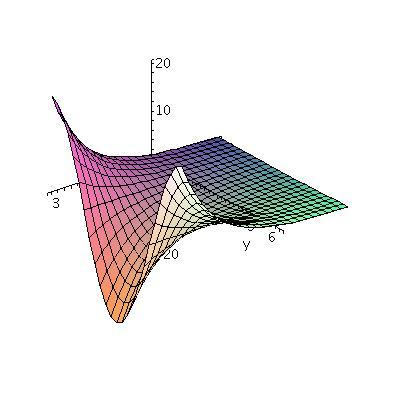
HOMEWORK
Please read carefully Chapter 1 of the text.
Please hand in these problems on Thursday, February 10:
1.5: 4, 8, 9, 19
Also please answer the following question:
One definition of a^b is exp(b log a) (in this course we will use the complex analysis meanings of exp and log!). Use this definition to find all possible values of iⁱ, 2², i², and 2ⁱ.

Comment The problem is "easy" but irritating. Maple could help you with part of it. For example, the command evalf(I^I); gets the response .2078795764 which might be an approximation to part of one answer above. Note, though, that I'd like exact answers in terms of traditional mathematical constants and values of calc 1 functions, not approximations.

1.6: 1, 2, 4, 5

 x+iy     (x+iy)(x+iy)    (x2-y2)       2xy
------ = ------------- = -------- + i ------
 x-iy     (x-iy)(x+iy)    (x2+y2)     (x2+y2)

HOMEWORK
Please hand in these problems on Thursday:
1.4: 1, 2, 15, 19, 36. This is a small assignment. In the future I hope to give assignments on Thursday to be handed in a week later.
Reminder Starting on Thursday, February 3, the class will meet in Hill 423.

I reviewed convergence of an infinite sequence introduced last time and made a very poor pedagogical decision. I decided to state the Cauchy Criterion for convergence of a sequence. I tried to motivate this in several ways. First, the definition of a convergent series used the limit of the sequence as part of the defintion. I wanted to show students that there could be an "internal" condition, only referring to the terms of a sequence itself, which would be equivalent to convergence. But I ignored my own exprience, much of it obtained by teaching Math 311. This experience showed that developing and understanding the Cauchy criterion for convergence takes most people weeks of struggle (and some students seem hardly able to understand it even then!). So I talked "around" the Cauchy Criterion for a while, and then finally stated it:
A sequence {z_n} satisfies the Cauchy Criterion if and only if for every epsilon>0, there is a positive integer N *usually depending on epsilon) so that for n and m >=N, |z_n-z_m|<epsilon.

Any sequence which converges satisfies the Cauchy Criterion, because the terms, when they are "far out" all get close to the limit of the sequence, and thus, by the Triaqngle Inequality, they get close to each other. That the converse is also true is not obvious, as I mentioned above, and several weeks of discussion in Math 311 are devoted to this converse.

The reason for the digression which was the mention of the Cauchy Criterion has to do with convergence of series. I defined the partial sum of a series, and as usual defined the convergence of an infinite series to be the limit of the sequence of partial sums, if such a limit existed. Then I remarked that a (non-zero!) geometric series would converge if the (constant) ration between successive terms had modulus less than 1. I could even then write a formula for the sum of such a series.

Most series do not have constant ratios between successive terms, and are not geometric series. The simplest way to test them for convergence is to use absolute convergence. A series converges absolutely if the series consisting of the moduli of the original series converges. This fact uses the Cauchy Criterion, and I should have followed the textbook, which cleverly sidesteps the Cuachy Criterion by mentioning that a complex series converges if and only if the real and imaginary parts converge, and then uses the real form of the comparison test to develop the result just quoted. This would have been much better!

A function f is continuous if f takes convergent sequences to convergent sequences.

We're almost at complex analysis. I'll get a version of the Intermediate Value Theorem next time, and then start differentiating.

      Rotation              Dilation
 
( cos(theta) -sin(theta) )   ( r  0 )
(                        )   (      )
( sin(theta)  cos(theta) )   ( 0  r )