Information for Maple assignment 3, spring 2006


This link describes the third Maple assignment.
Each student will get individual data by e-mail for the assignment.
The assignment is due Wednesday, April 5.


Where to find ...
      Pictures of degree two polynomials in two variables
      General information about conic sections
      Pictures of degree two polynomials in three variables
      Pictures of normal vectors to surfaces and how to draw them
      Pictures of normal vectors to curves and how to draw them


Ax2+Bxy+Cy2+Dx+Ey+F=0

What possible two-dimensional pictures can result from such an equation? Here are some examples. Nothing
This might be the most disturbing "picture". The equation x2+y2+1=0 is not satisfied by any pairs of numbers, (x,y), since the right-hand side is always positive. (Maybe this is an advertisement for complex numbers?)
One point
Look at 29x2+2xy+10y2+8x+12y+4=0. Then realize this is the same as (5x-y)2+(2x+3y+2)2=0 because (5x-y)2=25x2-10xy+y2 and (2x+3y+2)2=4x2+9y2+4+12xy+8x+12y. I did this in reverse, actually, and started with the squares. But the only way that (5x-y)2+(2x+3y+2)2 can be 0 is if (squares are never negative!) 5x-y=0 and 2x+3y+2=0. The first equation gives y=5x and when substituted in the second equation you get 2x+3(5x)+2=0 so that x=-2/17 and then y=-10/17. So "clearly" (not so clearly to me!) the point (-2/17,-10,17) is the only solution to 29x2+2xy+10y2+8x+12y+4=0.
A straight line
Just x+y=0 will do.
A circle, or its squeezed relative, an ellipse
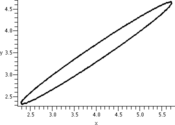
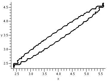
Certainly students should recognize x2+2y2-1=0 as an ellipse. But you may find it difficult to believe that 11x2-32xy+24y2+24x-40y+21=0 is also an ellipse. You could try the Maple command
implicitplot(11*x^2-32*x*y+24*y^2+24*x-40*y+21=0, x=1..6, y=2..5, scaling=constrained, thickness=2, color=black, grid=[100,100]);
and see the result. Most of the options to this command should be familiar (the thickness and scaling, for example). One option which might be new is grid. The default for the implicit plot command is to check on a 25 by 25 grid (that's 625 points). Requesting more points will usually give a smoother picture. Of course, the grid=[100,100] requires 42=16 times as much computation. On my home PC, the [25,25] grid took about .064 seconds and the [100,100] grid took about .72 seconds.
With grid=[100,100]
No specification, so grid=[25,25]
A parabola
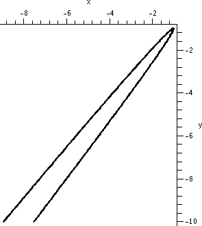
One simple example is x2+y=0. And, again, it may not be obvious that 25x2-40xy+16y2+13x-9y+3=0 is also a parabola, but displayed to the right is the result of this Maple command: implicitplot(25*x^2-40*x*y+16*y^2+13*x-9*y+3=0, x=-10..0, y=-10..0, scaling=constrained, thickness=2, color=black, grid=[100,100]);
Hyperbola
The model hyperbolas you have been told about include xy=1 and x2-y2=1.
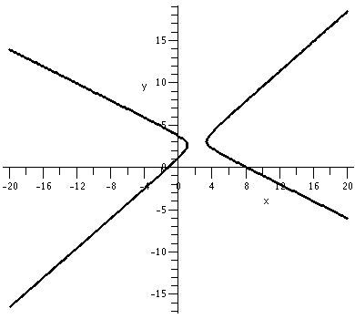
But -7x2-6xy+16y2+48x-80y+74=0 is also the equation of a hyperbola whose graph is shown to the right.
"Degenerate" hyperbolas
Well, xy=0 is sort of a hyperbola. It is (sigh!) a degenerate hyperbola or limiting form of a hyperbola. For example, xy=0 is a pair of lines which intersect in one point, and this "curve" is certainly the limit of the curves xy=tiny number as tiny number-->0. Also two parallel lines can be described by a quadratic polynomial: the points (x,y) which satisfy x2=1 are the straight lines x=1 and x=-1. This is another "degenerate" case.
All of these curves are called conic sections.


What are conic sections and why should I care?

We need to build a right circular cone. This is a cone with a central axis perpendicular to a plane.

Step 1
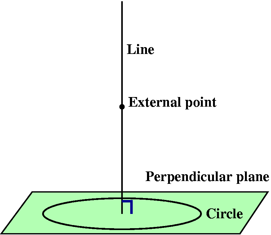
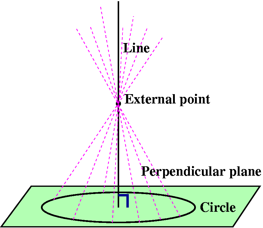
Take a straight line (which will be the axis of symmetry of the cone), and take a plane perpendicular to the line. In the plane, imagine a circle whose center is the point of intersection of the line and the plane. Now fix a point on the line outside of the plane.
Step 2
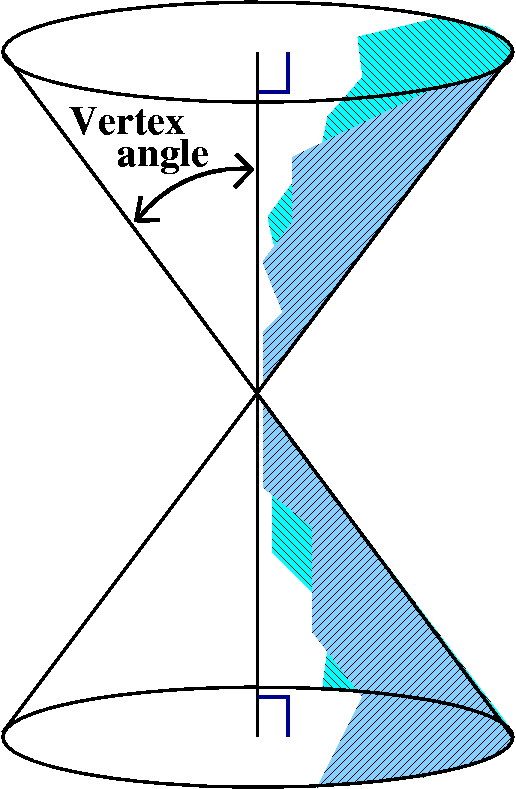
Now draw a straight line through the external point and every point on the circle. This collection of lines will form a surface. Each of the lines is called a generator of the cone. The original line is the axis of symmetry of the cone. The external point is called the vertex of the cone.
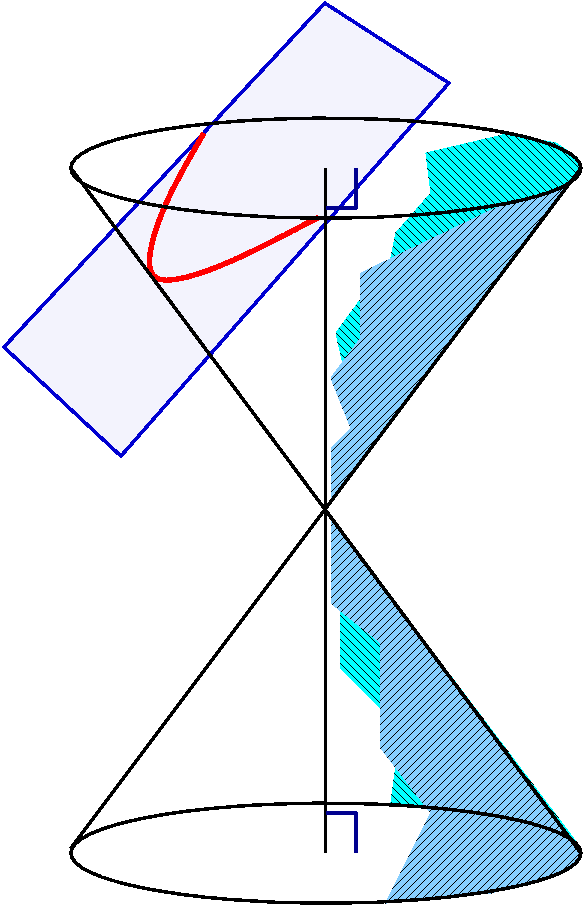
The right circular cone looks like what is sketched to the right. Suppose this cone is sliced by another plane. A conic section is the resulting curve: the intersection of the cone and the plane. The type of the curve is determined by the angle made by the intersecting plane and the axis, and how this angle relates to the vertex angle of the cone.
Ellipse

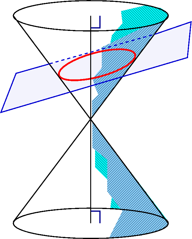
If the angle made by the intersecting plane and the axis is greater than the vertex angle, then the plane will only slice through one of the cone's pieces. The resulting curve is an ellipse.

Hyperbola

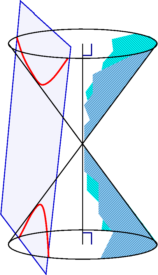
If the angle made by the intersecting plane and the axis is less than the vertex angle (or is parallel to the axis of symmetry), then the plane will slice through both parts of the cone's pieces. The resulting curve is a hyperbola.

Parabola

If the intersecting plane is exactly parallel to one of the generating lines (and that's darn unlikely for a random plane!) then it will slice through only one part of the cone. The resulting curve is a parabola.

These geometric characterizations of the conic sections are thousands of years old. There are also definitions of the various conic sections using distance in the plane. For example, an ellipse is the collection of points the sum of whose distances to two fixed points is a constant.

Applications
If the universe were empty except for the sun (a heavy point mass) and an asteriod (a much lighter mass) than the orbit the asteroid would have around the sun would be a conic section. The textbook discusses this in the section on Kepler's laws. So these curves (motion in an inverse square law force field) will be everywhere in physics.


Algebraic characterization of the conic sections

Suppose we want to know which conic section is given by Ax2+Bxy+Cy2+Dx+Ey+F=0. I'll assume that |A|+|B|+|C|>0, so that at least one of the quadratic coefficients is not 0. Otherwise we've just got a line or a point. The type of the curve depends on the discriminant. The discriminant is defined to be B2-4AC.

If B2-4AC<0 then the curve is an ellipse.
We looked at the ellipse 11x2-32xy+24y2+24x-40y+21=0 earlier, with A=11, B=-32, and C=24. The (-32)2-4(11)(24) turns out to be -32.

If B2-4AC>0 then the curve is a hyperbola.
An example of a hyperbola earlier was -7x2-6xy+16y2+48x-80y+74=0. Here A=-7, B=-6, and C=16, so B2-4AC=(-6)2-4(-7)(16)=484>0.

If B2-4AC=0 then the curve is a parabola.
I had claimed earlier that 25x2-40xy+16y2+13x-9y+3=0 was a parabola. Here(-40)2-4(25)(16)=0.

These algebraic statements are several hundred years also, and can be verified using high school algebra, but I'll admit the high school algebra must be applied very diligently. Some students might see a resemblance in the discriminant analysis and consequences to the second derivative test for functions of two variables, and the resemblance is not accidental. The second derivative test actually uses these results in a somewhat disguised form, where the Ax2+Bxy+Cy2+Dx+Ey+F is the second order Taylor polynomial of the function. The complexity of the three variable pictures below indicate how complicated second derivative tests in three variables must be.


What happens in three variables? Here there are more models, and things are more complicated. The general form is

Ax2+By2+Cz2+Dxy+Exz+Fyz+Gx+Hy+Iz+J=0

and there are ten coefficients. What can we get?

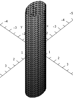
Here is an elliptical cylinder: x2+2y2-1=0. There's no z mentioned, so we take the ellipse in the xy-plane and just move it up and down in the z direction any distance desired.

The Maple command
implicitplot3d(x^2+2*y^2=1, x=-5..5, y=-5..5, z=-5..5, grid=[40,40,40], axes=normal, labels=[x,y,z]) produces the picture shown.
Notice that the grid option now has three entries, and therefore doubling the entries will require about eight times more "work" -- you should expect much more time to be needed if the grid entries are high.

Here is a cylinder over a hyperbola:
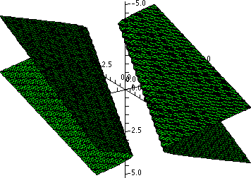
x2+z2-2y2-2xz-12yz+9z2-1=0

How do I "know" this? Well, I got this by expanding the following:
(x-z)2-2*(y+3*z)2=1
and I hope you can see the source for the hyperbola, which is x2-2y2=1. Then I altered the hyperbola equation by changing x to x-z and y to y+3z. The result is an oblique (tilted!) cylinder over a hyperbola.

The Maple command
implicitplot3d((x-z)^2-2*(y+3*z)^2=1, x=-5..5, y=-5..5, z=-5..5, grid=[60,60,60], axes=normal, labels=[x,y,z]) produces the picture shown.

So far these polynomials and their graphs really come from two dimensions. What can we have that's different from cylinders and points and lines?

New, three-dimensional stuff

  • Ellipsoid
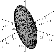
    Well, maybe this isn't too new. An ellipsoid is the three-dimensional analogue of the ellipse. Here is an equation for one ellipsoid
    (x-z)2+3(x-y)2+2(y+z)2=1
    and to the right is a picture of it.
  • Elliptical paraboloid
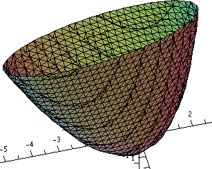
    The simplest paraboloid is z=x2+y2, a sort of cup. Here is a disguised elliptical paraboloid and its picture:
    (x-z)2+5z2+2(y+z)=1.
  • Hyperbolic paraboloid (or saddle)
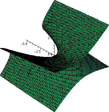
    The prototype here is z=x2-y2. The sections with z=constant are hyperbolas and the sections with x or y=constant are parabolas. This can be a bit confusing when you see one that is disguised. For example, let me just take the previous example, and change one sign:
    (x-z)2-5z2+2(y+z)=1
    This saddle is sitting sideways.
  • Hyperboloids
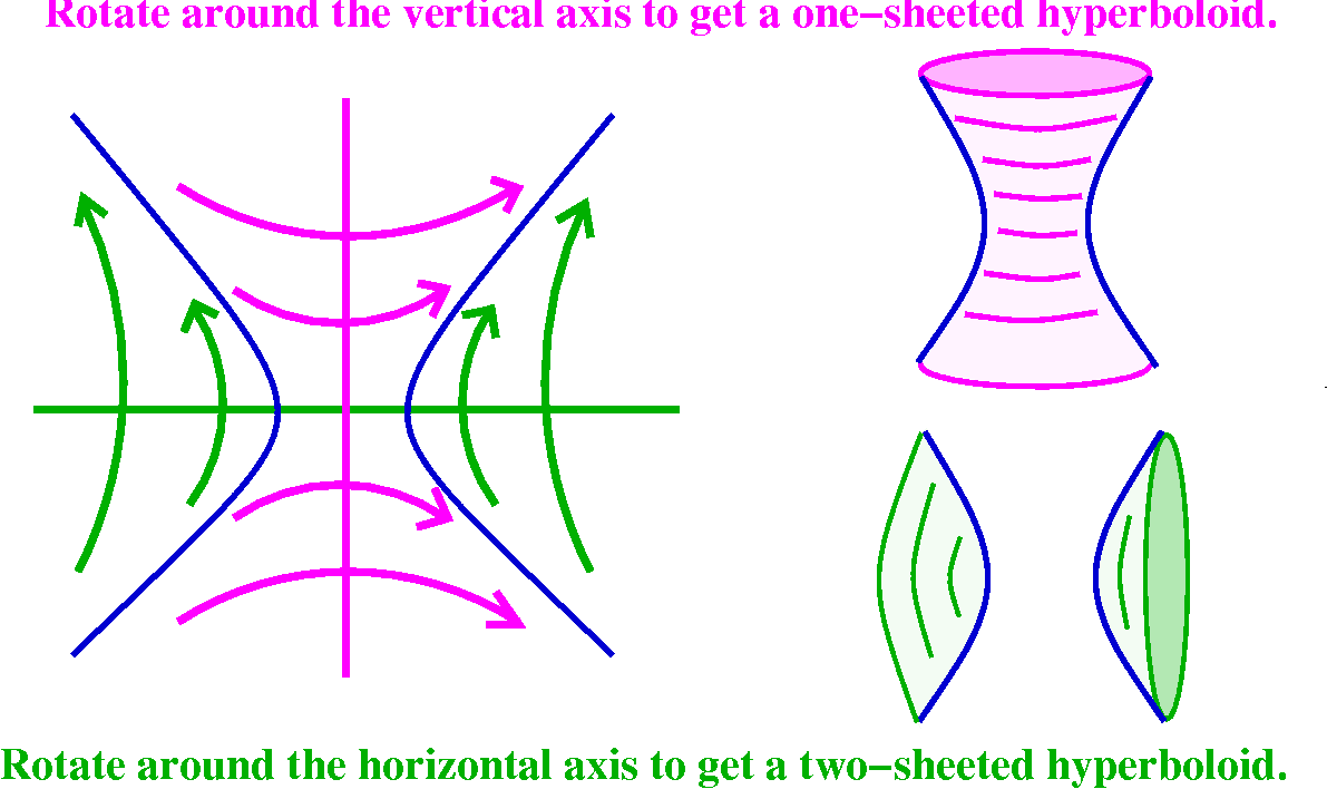
    In three dimensions there are two different analogues of hyperbolas.
    The word "sheet" is used in an antique, specialized sense with surfaces: it means one connected "piece" of a surface. So a hyperboloid with one sheet is a surface with one (connected) piece, and a hyperboloid with two sheets is a surface with two (connected) pieces. The Oxford English Dictionary gives this definition with a citation from 1827: "A portion of a surface analogous to the branch of a curve." Of course this is definition #11 for "sheet" and there are many other definitions for the word.

    Hyperboloid of one sheet
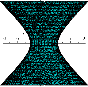
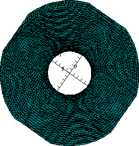
    The prototype here is x2+y2=1+z2. I show two pictures of this because it may be hard to "see" and understand. Slices with z=constant are circles with centers on the z-axis, and for large positive and negative values of z the circles get large. The circle of smallest radius is on the xy-plane. The radius is 1. The surface is connected but there is a hole in it. Please try to ignore the crinkles on the edges which are caused by the implicitplot3d command.

    Oblique (tilted) view Sideways view Top view

    Hyperboloid of two sheets
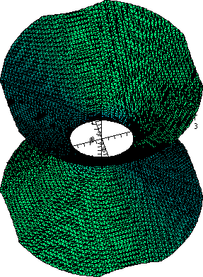
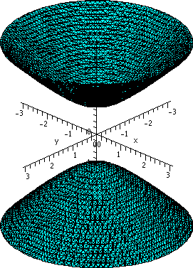
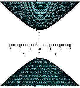
    The prototype here is x2+y2=z2-1. Notice that if z is between -1 and +1, then z2-1 is negative, so there will be no values of x and y with x2+y2 equal to z2-1. So this surface has two pieces, one above the xyu-plane, and one below the xy-plane. Here again are displayed two pictures of this surface. Slices with z=constant are circles with centers on the z-axis, and for large positive and negative values of z the circles get large. The circle(s) of smallest radius are when z=+/-1, and the circle then has radius 0 and is a point.

    Oblique (tilted) view Sideways view

  • The textbook has some similar pictures (see section 12.6, especially the table on page 836). The hyperboloid of two sheets always sits inside a cone, and the one-sheeted version sits outside a cone. Maybe you can "see" these cones if you rotate the lines which are the asymptotes for the original hyperbola.


    How to draw a normal vector

    For surfaces
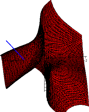
    I invented the function F(x,y,z)=x3+5xz-y3+y. The point (1,0,0) is on the level surface F(x,y,z)=1. The gradient vector is perpendicular to the level surface. I've attempted to give some helpful comments in the text to the right of boxes in this color.

    
    > F:=x^3+5*x*z-y^3+y;
                                                  3            3
                                            F := x  + 5 x z - y  + y
    
                                     The surface is not familiar to me. I really wrote something weird, at random. Since there are terms of degree greater than 2, certainly I don't expect anything nice or familiar.
    
    > subs({x=1,y=0,z=0},F);
                                                       1
    
                                     Here I'm "plugging" in values for F's variables, and verifying that F(1,0,0)=1, so that (1,0,0) is on the surface defined by F(x,y,z)=1.
    
    > Fx:=diff(F,x);
                                                         2
                                                Fx := 3 x  + 5 z
    > Fy:=diff(F,y);
                                                          2
                                                Fy := -3 y  + 1
    > Fz:=diff(F,z);
                                                   Fz := 5 x
    > subs({x=1,y=0,z=0},Fx);
                                                       3
    > subs({x=1,y=0,z=0},Fy);
                                                       1
    > subs({x=1,y=0,z=0},Fz);
                                                       5
    > T:=spacecurve(<3*t+1,1*t,5*t>,t=0..(.3),color=blue,thickness=3,
          axes=normal);
    
                                     Here are computations of partial derivatives, and evaluations of the partial derivatives. The gradient of F at (1,0,0) is (3,1,5), so that the spacecurve command draws a short line segment starting at (1,0,0) in the direction of the gradient vector.
    
    > S:=implicitplot3d(F, x=-2..2, y=-2..2, z=-2..2, axes=normal, labels=[x,y,z],
           grid=[50,50,50], color=red);
    
    > display({S,T}};
    
                                     The implicitplot3d command draws the surface. Specifying that grid=[50,50,50] means that we should get a better picture than the default, but Maple must check 503=125,000 points in R3 and this command took about 2 seconds on my home PC.
    Below is the picture that resulted from displaying the normal vector and the piece of the surface together.
                                     What if I wanted to find the normal vector for some point that isn't as "nice" as (1,0,0)? Suppose I changed x, say, from 1 to .95, and z from 0 to -.15. What y values could I get? Here's one way to have Maple approximate the answers.
    
    > fsolve(subs({x=.95,z=-.15},F=1));
                                                  -1.289608097
    
    > Q:={x=.95,y=-1.289608097,z=-.15};
                                  Q := {x = 0.95, z = -0.15, y = -1.289608097}
    
    > subs(Q,F);
                                                  1.000000000
    
    > m1:=subs(Q,Fx);m2:=subs(Q,Fy);m3:=subs(Q,Fz);
                                                  m1 := 1.9575
    
                                               m2 := -3.989267132
    
                                                   m3 := 4.75
    
    > T1:=spacecurve(<m1*t+.95,m2*t-1.289608097,m3*t-.15>,t=0..(.3), 
          color=blue,thickness=3, axes=normal);
    
    > display({S,T,T1}};
    
                                     The first command, fsolve, asks for numerical solutions of F(x,y,z)=1 after substitution of the x and z values. The fsolve command can return more than one answer.
    I defined Q so that I would not have to type too much later. I substituted Q in F so that I could check fsolve's answer. Generally the answer should check to within the accuracy of Digits (the default accuracy is 10 decimal places).
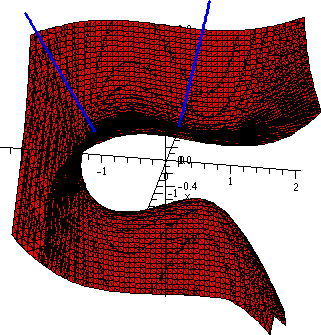
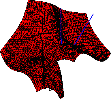
    Then I used Q and the previously computed partial derivatives to get the gradient at the new point. The spacecurve command created a new line segment in the direction <m1,m2,m3> starting at Q and finally display({S,T,T1}) showed a neat picture. Two views of the picture are below. In the left-hand view, I tried to show that the vectors were perpendicular to the surface: this view is from the side of the vectors. The other view is an attempt to show "things" in perspective.


    How to draw a normal vector

    For curves

    
    > F:=x^5-3*x*y^2+4*x+2*y;
                                                   5        2
                                             F := x  - 3 x y  + 4 x + 2 y
    
    > subs({x=1,y=2},F);
                                                       -3
    
    > Fx:=diff(F,x);Fy:=diff(F,y);
                                                      4      2
                                             Fx := 5 x  - 3 y  + 4
    
                                                Fy := -6 x y + 2
    
    > m1:=subs({x=1,y=2},Fx);m2:=subs({x=1,y=2},Fy);
                                                    m1 := -3
    
                                                   m2 := -10
    
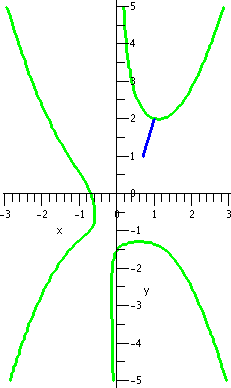
                                     I invented the function F(x,y)=x5-3xy2+4x+2y. Then I verified that F(1,2)=-3. I computed the partial derivatives, and now I know that the gradient of F at (1,2) is <-3,-10>.
    
    
    > T:=plot([-3*t+1,-10*t+2,t=0..(.1)],color=blue,thickness=2);
    
    > S:=implicitplot(F=-3, x=-5..5,y=-5..5, thickness=2, scaling=constrained, 
            color=green, grid=[50,50]);
    
    > display({S,T});
                                     If the option scaling=constrained is omitted from the implicitplot instruction, the normal vector doesn't appear to be correct. (I spent 10 minutes figuring this out, darn it!)
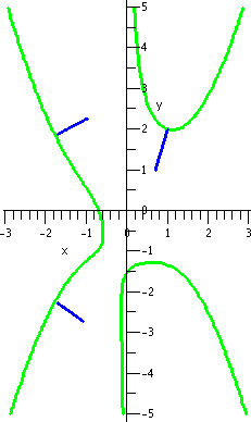
    Look at the picture. If x=-1.72, there are two values of y which will put (-1.72,y) on the curve. Maple can approximate these values, and then it can find and graph representations of the normal vectors at these points.
    Added 4/1/2006 I thank Ms. Caroline Pisacka for showing me some inaccuracies in past versions of the previous several commands.
    
    > fsolve(subs(x=-1.72,F));
                                           -2.264611822, 1.877014923
    
    > Q1:={x=-1.72,y=-2.264611822};Q2:={x=-1.72,y=1.877014923};
                                      Q1 := {x = -1.72, y = -2.264611822}
    
                                       Q2 := {x = -1.72, y = 1.877014923}
    
    > v1:=subs(Q1,Fx);v2:=subs(Q1,Fy);w1:=subs(Q2,Fx);w2:=subs(Q2,Fy);
                                               v1 := 32.37525269
    
                                               v2 := -23.37079400
    
                                               w1 := 37.19109774
    
                                               w2 := 19.37079401
    
    > yn:=-2.264611822; yp:=1.877014923;
                                               yn := -2.264611822
    
                                               yp := 1.877014923
    
    > Tn:=plot([v1*t-1.72,v2*t+yn,t=0..(.02),color=blue,thickness=2);
    
    > Tp:=plot([w1*t-1.72,w2*t+yp,t=0..(.02),color=blue,thickness=2);
    
    > display({S,T,Tn,Tp});
                                     I wrote the assignment statements (that is, using := to give values to variables) because I didn't want to keep entering the numbers or using my mouse to copy them. I will admit with two points and two normal vectors, keeping everying "straight" (correct) can be difficult. Also, I had to play with the plot statements (the range of the variable t, in particular) to get things to look good.


    Maintained by greenfie@math.rutgers.edu and last modified 3/20/2006.