Information for Maple assignment 1, spring 2006
This link describes the first
Maple assignment.
Each student will get individual data by
e-mail for the assignment.
The assignment is due February 1.
Here is some help for the first formal Maple assignment. The
assignment requests several pictures.
Pictures are
very important. Not many people can get much information from vast
tables of numbers, but humans possess a large capacity to receive and
organize visual information.
You are allowed and, indeed,
encouraged to copy and modify the commands discussed here.
Many useful packages can be loaded after Maple is "turned
on". One package contains several three dimensional plotting
commands. Please try the following command in Maple:
>with(plots);
and see a large number of commands appear which are now easily
accessible. One of them is spacecurve. To see more about this
command you can type
>help(spacecurve);
| Beginning pictures |
|---|
The command
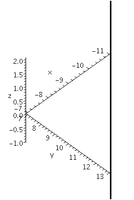
>spacecurve([4*t-11,3*t+7,-5*t+2],t=0..1,axes=normal,color=black,thickness=2,labels=[x,y,z]);
draws a line segment from the point (-11,7,2) where t=0, to the point
(-7,10,-3) where t=1. The picture Maple displays is shown below and
it is deceptive. The line segment is not
vertical although it is shown that way. The axes shown do not have
equal spacing which distorts the picture even more.
|

|
Change the command to
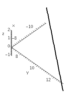
>spacecurve([4*t-11,3*t+7,-5*t+2],t=0..1,axes=normal,color=black,thickness=2,labels=[x,y,z],
scaling=constrained);
The result is shown below. All the axes now have
the same scale, and the line segment is no longer displayed vertically.
|

|
The command
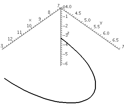
>spacecurve([3*cos(t)+10,3*sin(t)+4,-3],t=0..Pi,axes=normal,color=black,thickness=2,
labels=[x,y,z]);
asks for a picture of a semicircle of radius 3 centered at
(-10,-4,-3) in the plane z=-3. This view is
unconstrained. The result seems to be a
parabolic arc because Maple attempts to stretch the curve to fill up
the viewing window as much as possible.
|

|
Change the command to
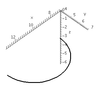
>spacecurve([3*cos(t)+10,3*sin(t)+4,-3],t=0..Pi,axes=normal,color=black,thickness=2,
labels=[x,y,z],scaling=constrained);
The result is shown below. The curve seems much more like a semicircle.
|

|
The image can be manipulated in various ways before "exporting" or
printing it. It can be rotated, scaled, etc. with some mouse clicks
on the picture. Below the images above will be displayed
together in various ways.
>A:=spacecurve([4*t-11,3*t+7,-5*t+2],t=0..1,axes=normal,color=black,thickness=2,labels=[x,y,z],scaling=constrained):
>B:=spacecurve([3*cos(t)+10,3*sin(t)+4,-3],t=0..Pi,axes=normal,color=black,thickness=2,labels=[x,y,z],scaling=constrained):
>display3d({A, B});
The first two commands assign values to the variables A and
B. The values are the plots. The display3d command
shows the plots together.
| More pictures |
|---|
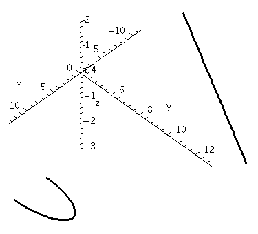
| This is the result with scaling=unconstrained.
|

|
| This is the result with scaling=constrained.
|

|
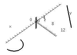
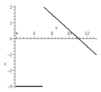
| Here is a a very bad version of the picture. It is
taken from "the side", with the x-axis coming straight out of the
image. This picture seems to show two line segments.
|

|
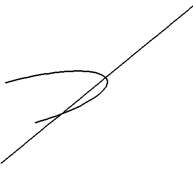
| Here's another very bad version of the picture. The
axes have been taken away, and the viewing angle makes the line
segment seem to cross what could be a parabolic arc.
|

|
The point of showing very bad versions of
the pictures is to try to emphasize that the graphs can actually
impair technical communication instead of helping.
Now we analyze more vectors and show more pictures.
Suppose p is the point (3,10,-7), q is the point (9,8,3), and r
is the point (6,5,7).
>[9,8,3]-[3,10,-7];
                                  [6, -2, 10]
This is the vector from p to q. A picture of the vector can be saved with
the command
>AA:=spacecurve([6*t+3,-2*t+10,10*t-7],t=0..1,axes=normal,color=black,thickness=2,labels=[x,y,z],scaling=constrained);
A similar computation gets the vector from p to r and the corresponding picture:
>[6,5,7]-[3,10,-7];
                                  [3, -5, 14]
>BB:=spacecurve([3*t+3,-5*t+10,14*t-7],t=0..1,axes=normal,color=black,thickness=2,labels=[x,y,z],scaling=constrained);
What about the cross product of the two vectors? The following
commands compute the cross product:
>with(VectorCalculus):
>SetCoordinates('cartesian'[x,y,z]):
><6,-2,10>&x<3,-5,14>;
                             22 e  - 54 e  - 24 e
                                 x       y       z
Then the cross product, as a vector "based" at p, can be drawn:
>CC:=spacecurve([22*t+3,-54*t+10,-24*t-7],t=0..1,axes=normal,color=black,thickness=2,labels=[x,y,z],scaling=constrained);
and all of the pictures can be displayed with
>display3d({AA,BB,CC});
| Even more pictures |
|---|
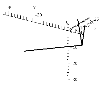
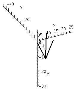
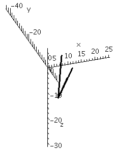
| Here's a picture of the three vectors, all based at the point
p. I have rotated the picture and attempted to show that the cross
product appears perpendicular to the other two vectors.
|

|
| Here's a very bad version of the picture. I managed to
get a view of the three vectors which bunches them all together, and
obscures the geometry, both the angles and the lenghts. This is not useful!
|

|
| Here's another very bad version of the picture, which
needed an even more careful view. A casual glance will see only two
vectors. Don't do this!
|

|
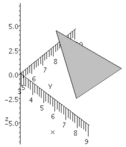
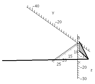
Here is a picture of the triangle in R3 whose
vertices are the points p and q and r. This picture is very easy to
create using a command in the plots package. Find this
command yourself: look at the list of commands in plots and
guess and then use help.
By the way, by rotating the viewpoint, you can make any of the
angles of this triangle seem to be a right angle! Perspective can be
deceptive and irritating.
|

|
Finally, here are the triangle, two of the vectors along the
triangle's edges, and the cross product of these two edge
vectors.
The view has been chosen so that the cross product
seems to be perpendicular to the triangle, which it is. Twice the area
of the triangle is equal to the length of the cross product.
|

|
Maintained by
greenfie@math.rutgers.edu and last modified 1/3/2006.
