A collection of examples

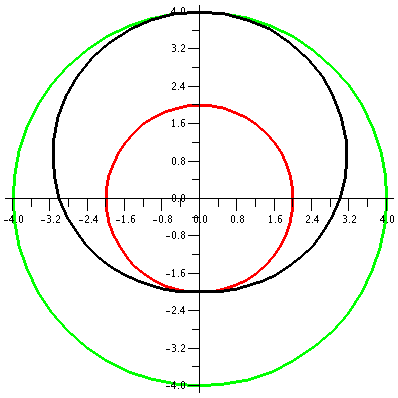
r=3+sin(θ) Let's consider r=3+sin(θ). Since the values of sine are all between -1 and 1, r will be between 2 and 4. Any points on this curve will have distance to the origin between 2 and 4 (the green and red circles on the accompanying graph). When θ=0 (the positive x-axis) r is 3. As θ increases in a counterclockwise fashion, the value of r increases to 4 in the first quadrant. In the second quadrant, r decreases from 4 to 3. In the third quadrant, corresponding the sine's behavior (decrease from 0 to -1) r decreases from 3 to 2. In all of this {in|de}crease discussion, the geometric effect is that the distance to the origin changes. We're in a situation where the central orientation is what matters, not up or down or left or right. Finally, in the fourth quadrant r increases from 2 to 3, and since sine is periodic with period 2Pi, the curve joins its earlier points. The picture to the right shows the curve in black. I'd describe the curve as a slightly flattened circle. The flattening is barely apparent to the eye, but if you examine the numbers, the up/down diameter of the curve is 6, and the left/right diameter is 6.4.
Converting to rectangular coordinates A naive person might think, "Well, I could convert the equation r=3+sin(θ) to rectangular coordinates and maybe understand it better." Except under rare circumstances (I'll show you one below), the converted equation is very irritating and difficult to understand. For example, Let's start with r=3+sin(θ) and multiply by r. The result is r2=3r+r·sin(θ). I multiplied by r so that I would get some stuff I'd recognize from the polar/rectangular conversion equations. r2 is x2+y2 and r·sin(θ) is y. So I have x2+y2=3r+y, or x2+y2-y=3r. I would rather avoid square roots so I will square this, and get (x2+y2-y)2=9r2=9(x2+y2). This is a polynomial equation in x and y of highest degree 4, defining this curve implicitly. I don't get much insight from this.
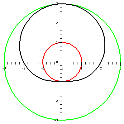
r=2+sin(θ) Now consider r=2+sin(θ). Again, the values of sine are all between -1 and 1, so r will be between 1 and 3. Any points on this curve will have distance to the origin between 1 and 3. We can begin (?) the curve at θ=0 when r=2, and spin around counterclockwise. The distance to the origin increases to r=3 at θ=Pi/2 (the positive y-axis). The distance to the origin decreases back to r=2 when θ=Pi (the negative x-axis). The curve gets closest to the origin when θ=3Pi/2 (the negative y-axis) when r=1. Finally, r increases (as θ increases in the counterclockwise fashion) to r=3 again when θ=2Pi. Here the "deviation" from circularity in the curve is certainly visible. The bottom seems especially dented.
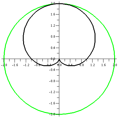
r=1+sin(θ) We decrease the constant a bit more, and look at r=1+sin(θ). The values of sine are all between -1 and 1, so r will be between 0 and 2. The (red) inner circle has shrunk to a point. This curve will be inside a circle of radius 2 centered at the origin. We begin our sweep of the curve at 0, when r is 1. Then r increases to 2, and the curve goes through the point (0,2). In the θ interval from Pi/2 to Pi, sin(θ) decreases from 1 to 0, and the curves moves closer to the origin as r decreases from 2 to 1. Something rather interesting now happens as θ travels from Pi to 3Pi/2 and then from 3Pi/2 to 2Pi. 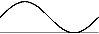The rectangular graph of 1+sine, shown here, decreases down to 0 and then increases to +1. The polar graph dips to 0 and then goes back up to 1. The dip to 0 in polar form is geometrically a sharp point! I used "!" here because I don't believe this behavior is easily anticipated. The technical name for the behavior when r=3Pi/2 is cusp. This curve is called a cardioid from the Latin for "heart" because if it is turned upside down, and if you squint a bit, maybe it sort of looks like the symbolic representation of a heart. Maybe.
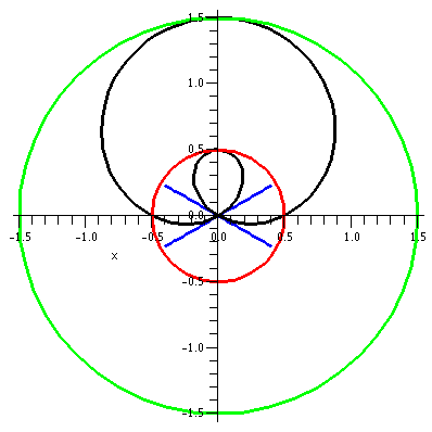
r=1/2+sin(θ) Let's consider r=1/2+sin(θ). The values of sine are all between -1 and 1, so r will be between -1/2 and 3/2. The (red) inner circle actually had "radius" -1/2, and it consists, of course, of points whose distance to the pole, (0,0), is 1/2. When θ is 0, r is 1/2. In the first two quadrants, 1/2+sin(θ) increases from 1/2 to 3/2 and then backs down to 1/2. In the second two quadrants, when θ is between Pi and 2Pi, more interesting things happen. The rectangular graph on the interval [0,2Pi] of sine moved up by 1/2 shows that this function is 0 at two values, and is negative between two values. The values are where 1/2+sin(θ)=0 or sin(θ)=-1/2. The values of θ satisfying that equation in the interval of interest are Pi+Pi/6 and 2Pi-Pi/6. The curves goes down to 0 distance from the origin at Pi+Pi/6, and then r is negative until 2Pi-Pi/6. The natural continuation of the curve does allow negative r's, and the curve moves "behind" the pole, making a little loop inside the big loop. Finally, at 2Pi-Pi/6, the values of r become positive, and the curve links up to the start of the big loop. This curve is called a limacon. The blue lines are lines with θ=Pi+Pi/2 and θ=2Pi-Pi/6. These lines, for the θ values which cross the pole, are actually tangent to the curve at the crossing points.
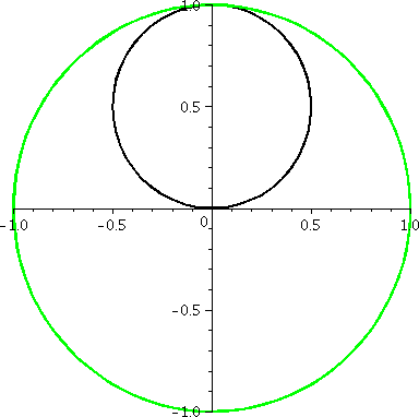
r=0+sin(θ) Let's try a last curve in this family, with the constant equal to 0. What does r=sin(θ) look like? A graph is shown to the right. There are several interesting features of this graph. First, this is a polar curve which does have a nice rectangular (xy) description. If we multiply r=sin(θ) by r, we get r2=r·sin(θ), so that x2+y2=y. This is x2+y2-y=0 or, completing the square, x2+y2-2(1/2)y+(1/2)2-(1/2)2=0 so that (x-0)2+(y-1/2)2=(1/2)2. This is a circle of radius 1/2 and center (0,1/2), exactly as it looks. The moving "picture" of this curve is quite different. Between 0 and π it spins once around the circle but then from π to 2π it goes around the circle another time! So this is really somehow two circles, even though it looks like only one geometrically.

More information about these curves is available here

Length of polar curves
The formula is ∫_θ=α^θ=βsqrt(r²+(dr/dθ)²)dθ. I used this to find the length of the cardioid above (the double angle formula from trig is needed). Then I used it to find the length of a circle (!), but here the novelty is that we actually trace the circle r=cos(θ) twice from 0 to 2π, so some care is needed if we only wanted to find the length of one circumference.

"Sketching" roses
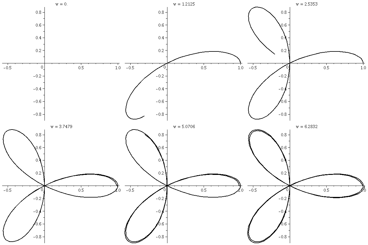
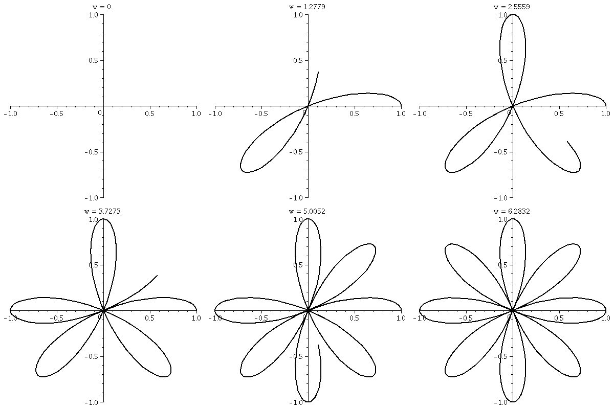
Here are dynamic pictures of two roses. The first is the one I sketched in class r=cos(3θ). It is covered twice and has 3 "petals". The second is r=cos(4θ). It is only covered once, and it has 8 petals! Wow, polar coordinates can be annoying!

r=cos(3) This is a three-leafed rose. Please note that the graph shows one sweep, as θ goes from 0 to 2Pi. The rectangular graph, shown here, has three pairs of ups and downs. The polar trace covers the leaves twice. The six up-and-downs of cos(3θ) (magically?) reduce to retracings of half of the loops. I hope I made this evident. I introduced some deliberate distortion in the second tracing. (!) Without the distortion, the second tracing could not be seen at all, since the pixels the "point" travels over and colors all had already been colored.

r=cos(4θ) This "rose" has 8 leaves or petals, and the dynamic way it is traced is weird and wonderful to me. The rectangular graph. to the right, shows four bumps up and four bumps down. There are no retracings of already colored points, so that the wiggles up and down of cos(4θ) all result in 8 leaves.

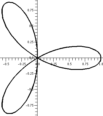Area inside one petal of r=cos(3θ)
Well, cos(3θ) "first" (going from 0 to 2π) is 0 when 3θ=π/2. So we get half a petal by integrating from 0 to π/6. The formula is ∫_α^β(1/2)r²dθ so this becomes (for the whole petal, we need to double):
2·(1/2)∫₀^π/6 cos(3θ)²dθ. We computed this using a trig identity. r=cos(3θ). Area inside one petal?

I didn't talk about Exponentials and snails, darn it!

Therefore when t=-1, dy/dx=(2)/(1/2)=4. The line goes through (1/2,0), so an equation for it is y=4(x-1/2).
Therefore when t=1, dy/dx=(2)/(-1/2)=-4. The line goes through (1/2,0), so an equation for it is y=-4(x-1/2).

I had Maple graph the parametric curve and the two lines just found (in green and blue. I then asked what the angle between the lines (the angle which encloses the x-axis). Then, I waited, as more seconds of the 21^st century ticked by. Some time (and more words later) we decided that the angle was 151.9 degrees. Hey, please remember that the slope of a line is the tangent of the angle that the line makes with the positive x-axis. Here the line y=4(x-1/2) and the positive x-axis have angle equal to arctan(4), approximately 1.326 radians. Double this is about 151.9 degrees. Hey: you have the machines. Please use them.

Uniform speed?
We developed a formula for speed. It was sqrt(f´(t)²+g´(t)²) where x=f(t) and y=g(t). For the circle x=5cos(t) and y=5sin(t), previously considered, we know dx/dt=-5sin(t) and dy/dt=5cos(t), so that (dx/dt)²+(dy/dt)²=25((sin(t))²+(cos(t))²)=25·1=25, so the speed, which is the square root, is always 5. So this is uniform circular motion: the word "uniform" here means that the speed is constant. (Notice, oh physics people, that I am not saying the velocity is constant and I am not saying that the acceleration is 0. Indeed, both of those statements are false. The direction of the velocity is changing, so the acceleration is not 0. We need to look at these quantities as vectors, and this will be done in Math 251.)

Nonuniform speed
Then I tried to analyze an ellipse we had parameterized earlier. It turns out that what I wrote and said in the last lecture was incorrect. I am sorry. So: we have x(t)=5cos(t) and y(t)=3sin(t) so dx/dt=-5sin(t) and dy/dt=3cos(t), and the speed is the square root of 25(sin(t))²+9(cos(t))²= 16(sin(t))²+9(sin(t))²+(cos(t))²= 16(sin(t))²+9. Sigh. The speed at time t is sqrt(16(sin(t))²+9). When t=0, the particle whose motion we are describing is at (5,0) and the speed is sqrt(9)=3 since sin(0)=0. When t=&pi/2, the particle is at (0,3) and the speed is sqrt(25)=5 since sin(&pi/2)=1. So certainly the particle is not moving at the same speed. Indeed, a graph of the speed, sqrt(16(sin(t))²+9), is shown to the right.

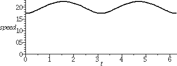Now this does resemble what I know about the motion of a planet in orbit. When it is far away from the center of the orbit, the planet will have large potential energy and relatively small kinetic energy (it will move slowly). This is near t=0 and t=π. When it is close to the center of the orbit, the planet moves faster, and the kinetic energy is larger, while the potential energy, measured by the work needed to move closer/farther from the center, decreases.
The total energy is conserved, but the way the total is divided between kinetic and potential energy varies. Maybe if you look again at the moving picture, you will see both of these phenomena. It is not too clear to me.

Length of a curve
Well, suppose we move along a parametric curve given by x=f(t) and y=g(t) from t=START to t=END. If we believe that the speed is sqrt(f´(t)²+g´(t)²), then we know that this speed can vary. In a sort time interval (dt long!) the distance traveled is Speed·Time, or sqrt(f´(t)²+g´(t)²)dt. We can add up all these distances from t=START to t=END using the integral idea. So the distance traveled along the curve from t=START to t=END will be given by ∫_t=START^t=ENDsqrt(f´(t)²+g´(t)²)dt. (We are integrating the magnitude of the velocity vector). Is this a reasonable formula?

Back to my favorite curve
The length of the loop in my favorite curve can be gotten by computing the integral of the speed from -1 to +1 (the two self-intersection times). So this is (I'll use the formulas we already have) ∫_-1¹sqrt((-2t/(1+t²)²)²+(3t²-1)²)dt. Maple takes more than half a second (quite a lot of time!) to acknowledge that it can't find an antiderivative, so we can't use FTC. In less than a tenth of a second, the approximate value 1.971944073 is reported.

Almost no speed functions have nice, neat, simple antiderivatives. In the real world, you'll need to use numerical approximation. However, Math 152 is not the real world.

A textbook problem
Section 11.3, problems 3 through 15, are all "Find the length of the path over the given interval" with some rather silly-looking functions specified. Accidentally (exactly not accidentally, actually!) all of the problems can be computed exactly with antiderivatives and values of standard functions. There is a fair amount of ingenuity involved in constructing such examples. I urged students to practice with several of them. I invited a suggest, and #7 was suggested. Here it is:
    Find the length of the path described by (3t²,4t³), 1≤t≤4.

The solution
Here x=3t² and y=4t³. We will compute the speed and then attempt to "integrate" (actually using FTC, so we'll need to find the antiderivative). Now dx/dt=6t and dy/dt=12t². Therefore the speed is sqrt(6t)²+(12t²)²). This is sqrt(36t²+144t⁴). We'll need to integrate this, and maybe I will "simplify" first. Indeed, since we consider t in an interval where t≥0, sqrt(t²)=t (otherwise we would need to worry about |t| or -t etc.). But 36t²+144t⁴=36t²(1+4t²) so that the square root is 6t·sqrt(1+4t²). Therefore the distance traveled along the curve is an integral, ∫_t=1^t=46t·sqrt(1+4t²)dt. Several students immediately suggested various substitutions. Here is one which does the job efficiently. So:     If u=1+4t², du=8t dt, so (1/8)du=dt.     ∫6t·sqrt(1+4t²)dt=(6/8)∫sqrt(u)du. The several errors made by the lecturer in class are not, I hope, duplicated here.
    Now (6/8)∫sqrt(u)du=(6/8)(2/3)u^3/2+C=(1/2)u+C=(1/2)(1+4t²)^3/2+C.
    So ∫_t=1^t=46t·sqrt(1+4t²)dt=(1/2)(1+4t²)^3/2|₁⁴=(1/2)(65)^3/2-(1/2)(5)^3/2.

The idea of polar coordinates
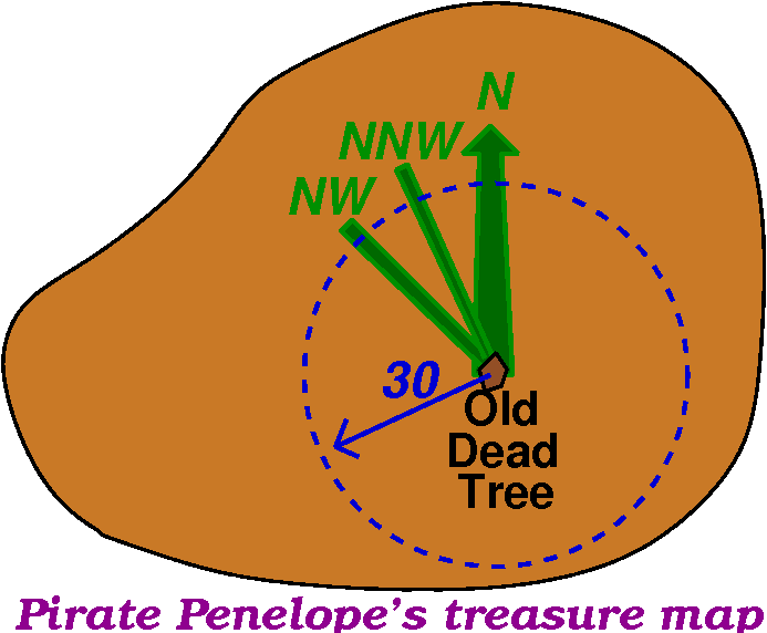
You have found a treasure map supposedly giving directions to the burial spot of a chest full of gold, jewels, mortgages, etc., stolen by the Dread Pirate Penelope. The information you have is that
A buried treasure is located 30 feet from the
old dead tree, in a NorthNorthWest direction.
So there you are, on the island. Perhaps the Old dead tree is still visible. You could mentally draw a circle 30 feet in radius around the Old Dead Tree. Then you find the North direction. π/4;=45^o to the West is NW (Northwest) and then NNW (Northnorthwest) is π/8 towards North (anyway, you decide on the direction). Where that direction intersects the circle is probably where to dig, unless Penelope is tricky, etc.

The whole idea of located a point in a 2-dimensional setting using distance from a fixed point and angle with respect to a fixed direction is called polar coordinates.

"Standard issue" polar coordinates
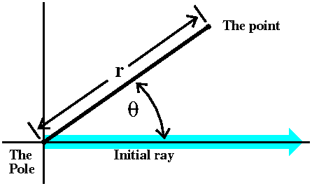Fix a point (usually called "the center" or sometimes "the pole" and in most common situations, the origin of the xy-coordinate system. Also fix a direction -- if need this might be called "the initial ray". Almost always this is the positive x-axis in an xy-coordinate system. Then locate another point in the plane by giving its distance from the center (called r) and by drawing the line segment between the center and the point you are locating. Measure the angle between that and the initial ray (note: counterclockwise is a positive angle!): this is called θ. r and θ are the polar coordinates of the point.

An example and the problem with polar coordinates
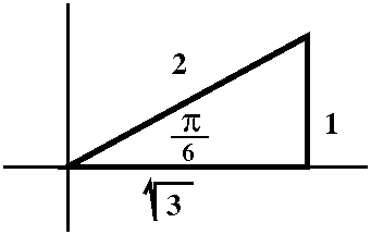Well, make the standard choices for "the pole" and "the initial ray". Let's get polar coordinates (the values of r and θ) for the point whose rectangular coordinates are x=sqrt(3) and y=1. Of course this is not a random point (sigh). So we consider the picture, and decide that the hypotenuse (r) should be 2 units long, and the acute angle (θ) should be π/6. Fine.

But suppose that the point (sqrt(3),1) is operating in a sort of dynamic way. Maybe it is the end of a robot arm, or something, and suppose that the arm is swinging around the pole, its angle increasing. It might be true that we somehow are computing various angles, and since the arm is moving continuously (still no teleporting robot arms!) the angles which are θ's should change continuously. If the arm swings completely around the pole, and comes back to the same geometric location, it would make more sense to report its polar coordinates as r=2 and θ=13π/6 (which is better understood as 2π+π/6).

Some valid polar coordinates for the point whose rectangular coordinates are x=sqrt(3) and y=1:
r=2 and θ=π/6 r=2 and θ=13π/6 r=2 and θ=25π/6 ETC.
But the "robot arm" could also swing around backwards, so other possible polar coordinates for the same geometric point include
r=2 and θ=-11π/6 r=2 and θ=-23π/6 ETC.
Generally, r=2 and θ=&pi/6+2π(multiplied by any integer): the integer could be 0 or positive or negative.

The irritation ("It's not a bug, it's a feature ...") is that there are further "reasonable" polar coordinate pairs for the same point! For example, go around to π/6+π. If you position your robot arm there, and then tell the arm to move backwards 2 units, the arm will be positioned at (sqrt(3),1). Sigh. So here are some more polar coordinates for the same point:
r=-2 and θ=7π/6 and r=-2 and θ=-19π/6 and r=-2 and θ=-31π/6 ETC.
but we are not done yet, because there are also (going backwards in the angle and the length)
r=-2 and θ=-5π/6 and r=-2 and θ=-17π/6 and r=-2 and θ=-29π/6 ETC.
Generally, r=-2 and θ=7&pi/6+2π(multiplied byany integer): the integer could be 0 or positive or negative.

Common restrictions on polar coordinates and the problems they have
This is irritating. Any point in the plane has infinitely many valid "polar coordinate addresses". In simple applications, people frequently try to reduce the difficulty. Much of the time, we expect r>0 always. And maybe we also make θ more calm. The restriction 0<θ<2π is used, except when it isn't, so the restriction -π<θ≤π is used in other circumstances. I am not trying to be even more incomprehensible than usual. I am merely reporting what different people do. As we will see, this is all very nice, except that there are natural circumstances, both in physical modeling (the robot arm I mentioned) and in the mathematical treatment, where it will make sense to ignore the artificial restrictions, even if this makes life more difficult. You'll see a few of these circumstances.

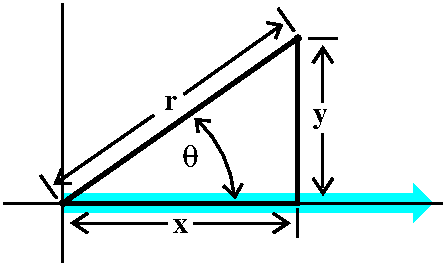
Conversion formulas
If you consider the picture to the right, I hope that you can fairly easily "read off" how to go from r and θ to x and y:
    x=r cos(θ)
    y=r sin(θ)
The lecturer made another embarrassing mistake here -- what's with him today?
Going from x and y to r is easy enough: r=sqrt(x²+y²). If we divide the y equation above by the x equation, the r's drop out and we get y/x=tan(θ) so that θ=arctan(y/x). Please note that there are infinitely many valid r and θ pairs for every point, so this method will only give you one such pair! Be careful in real applications, please.

Specifying regions in the plane in polar fashion
It is useful to try to get used to thinking in polar fashion, because then you will be able to see problems (usually physical or geometric problems with lots of central symmetry) where this coordinate system can be used to really simplify computations. So here are some simple examples of regions which can be easily specified with polar inequalities.

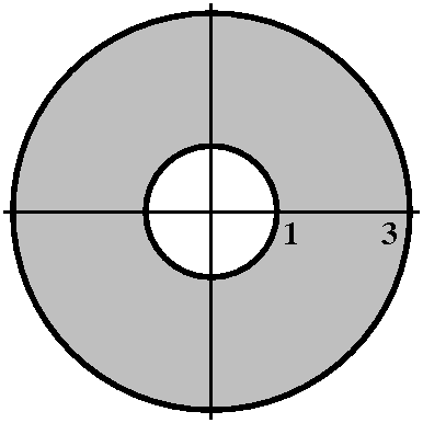
1<r<3 r=1 and r=3 represent two circles centered at 0, one of radius 1 and one of radius 3. The inequality, which has no restriction on θ, means that every point between these circles is in the region specified. This sort of region is frequently called an annulus.
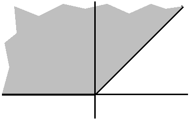
π/4<θ<π Here there is no restriction on r. I will assume (!!) the standard restriction that r should not be negative. Then a point is in this region if its angle with respect to the positive x-axis is more than π/4 and less than π (the angle π specifies the negative x-axis!!!). I guess I would call this region a wedge. I also "guess" that 0 is in this region. The wedge goes out radially "to infinity" in all of the legal θ directions.
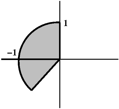
0<r<1 and π/2<θ<5&pi/4 Here are combined restrictions on both polar coordinates. I hope you can "see" the geometric result. I could describe this region in rectangular coordinates, certainly, but the needed equations and inequalities would be much more complicated to me. Maybe this sort of thing will give you some appreciation of the usefulness of polar coordinates.

We will study the equations and graphs of some polar curves next time, and we will do a bit of calculus (arc length and area). That will conclude the course lectures.

Parametric curves
We begin our rather abbreviated study of parametric curves. These curves are a rather clever way of displaying a great deal of information. Here both x and y are functions of a parameter. The parameter in your text is almost always called t. The simplest physical interpretation is that the equations describe the location of a point at time t, and therefore the equations describe the motion of a point as time changes. I hope the examples will make this more clear. The t here is usually described for beginners as time, but in applications things can get a great deal more complicated. Parametric curves could be used to display lots of information. I mentioned that some steels contain chromium. Maybe the properties of the steel such as ductility (a real word: "The ability to permit change of shape without fracture.") and density, might depend on the percentage of chromium. So the t could be that and the x and y could be measurements of some physical properties of the steel. Here x=f(t) and y=g(t), as in the text. Now a series of examples.

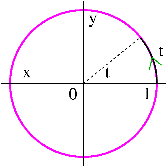Example 1
Suppose x(t)=cos(t) and y(t)=sin(t). I hope that you recognize almost immediately that x and y must satisfy the equation x²+y²=1, the standard unit circle, radius 1, center (0,0). But that's not all the information in the equations.

The point (x(t),y(t)) is on the unit circle. At "time t" (when the parameter is that specific value) the point has traveled a length of t on the unit circle's curve. The t value is also equal to the radian angular measurement of the arc. This is uniform circular motion. The point, as t goes from -infinity to +infinity, travels endlessly around the circle, at unit speed, in a positive, counterclockwise direction.

Example 2
Here is a sequence of (looks easy!) examples which I hope showed students that there is important dynamic (kinetic?) information in the parametric curve equations which should not be ignored.

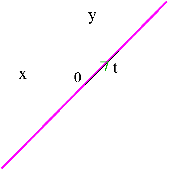
x(t)=t and y(t)=t. Surely the "particle" travels on the main diagonal line y=x. The travel (remember, the domain unless otherwise limited, is all values of t which makes sense to the defining functions) is from lower left (third quadrant) to upper right, (first quadrant). Also I hope that you see the particle moves at uniform speed. This is uniform linear motion.
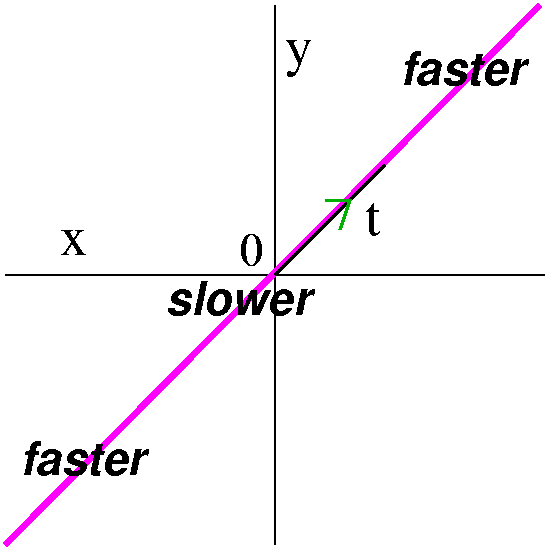
x(t)=t3 and y(t)=t3. The path of this point is also on the main diagonal line y=x. But the motion of this point, while in the same direction as the first example (from third to first quadrant), is very different. The difference is in the "clock". Try a few values of t. Between t=0 and t=1 we travel from (0,0) to (1,1). Between t=1 and t=2, we travel from (1,1) to (8,8). Just roughly, the distance changes from sqrt(2) to sqrt(98). That's a big change. The particle, near -infinity, travels fast. Then as t goes around 0, it is slower, and, as t gets very large positive, the particle moves faster.
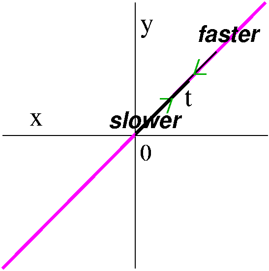
Now let's consider the motion described by x(t)=t2 and y(t)=t2. Again, we can "eliminate the parameter". That rather grim phrase (if you read murder mysteries!) is what the text uses to describe getting rid of t by manipulating the two equations. Here we just realize that x=y. Much of the information about the motion of this point on the main diagonal is lost if we go to just y=x. The t2 means that both x and y must be non-negative. When t is large negative, the point is way up high in the first quadrant, and traveling towards the origin rather rapidly. It begins to slow, and then "stops" (!) but only "instantaneously" (!!) at (0,0) (when t=0). It turns around (how the heck does a particle "turn around"?) and begins to retrace its path, up towards the open end (??) of the first quadrant. As it travels, its speed increases. So this is really quite complicated motion, and very different from the first two examples.
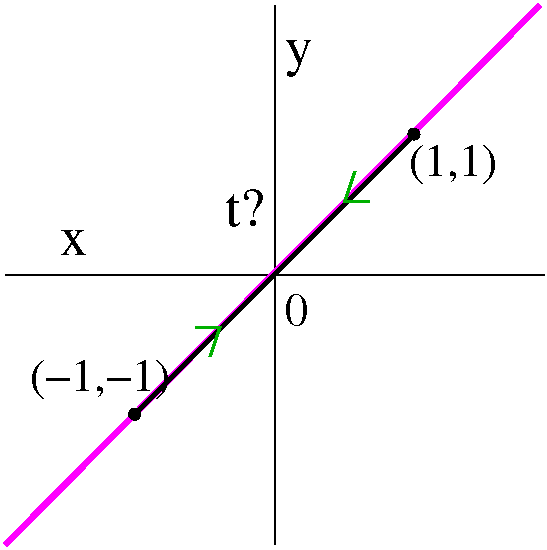
The final example in this series is x(t)=cos(t), and y(t)=cos(t). Again, the path traveled by the point is on the main diagonal line y=x. But now the dynoamics are extremely different. Because cosine oscillates endlessly between -1 and +1, the motion of the point whose position is described by these equations is on the line y=x and only between (-1,-1) and (1,1). It moves back and forth between these points, completing a round trip in every time interval of length 2Pi. This is very different motion from the other examples.

Example 3

I considered x(t)=5cos(t)and y(t)=5sin(t). This is a slight variant of the very first example. Since x(t)/5=cos(t) and y(t)/5=sin(t), I "know" that the particle's path must be on (x/5)2+(y/5)2=1, so x2+y2=52, a circle whose center is (0,0) and radius is 5. The fact that the path lies on the circle whose equation is given is fairly clear. But I was asked a slightly different question in class: why does the point travel in a counterclockwise direction? When you learn about velocity vectors, this may also be "fairly" clear, but right now, if you plug in t=0, the point (x(t),y(t)) is (5,0), and if you plug in π/2, the point is (0,5). Therefore I feel that travel proceeds in a counterclockwise direction, from (5,0) to (0,5) and so on.

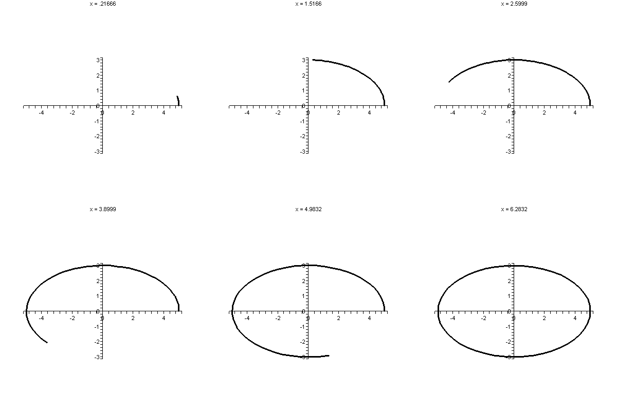
What if x(t)=5cos(t) and y(t)=3sin(t)? Then the trig identity gives (after elimination of the parameter) (x/5)2+(y/3)2=1 as the possible path of the point. This is an ellipse centered at (0,0). Its wider part (total length 1) is on the horizontal axis, as shown. The vertical extant of the ellipse is 6. So I attempted to create a moving image of this curve. I hope it is helpful to you. The parameterization is by central angle. Speed varies .... Originally, further comments followed, but these, it turns out, were incorrect. I apologize. See the next lecture's diary entry for more information.

A bug drawing out a thread ...
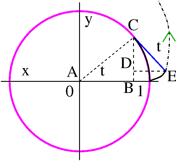Thread is wound around the unit circle centered at the origin. A bug starts at (1,0) and is attached to an end of the thread. The bug attempts to "escape" from the circle. The bug moves at unit speed.

I would like to find an expression for the coordinates of the bug at time t. Look at the diagram. The triangle ABC is a right triangle, and the acute angle at the origin has radian measure t. The hypotenuse has length 1, and therefore the "legs" are cos(t) (horizontal leg, AB) and sin(t) (vertical leg, BC). Since the line segment CE is the bug pulling away (!) from the circle, the line segment CE is tangent to the circle at C. But lines tangent to a circle are perpendicular to radial lines. So the angle ECA is a right angle. That means the angle ECD also has radian measure t. But the hypoteneuse of the triangle ECD has length t (yes, t appears as both angle measure and length measure!) so that the length of DE is t sin(t) and the length of CD is t cos(t).

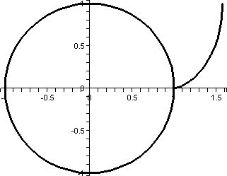
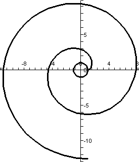
The coordinates of E can be gotten from the coordinates of C and the lengths of CD and DE. The x-coordinates add (look at the picture) and the y-coordinates are subtracted (look at the picture). Therefore the bug's path is given by x(t)=cos(t)+t sin(t) and y(t)=sin(t)-t cos(t).

t between 0 and 1	t between 0 and 10 Note that the scale is changed!

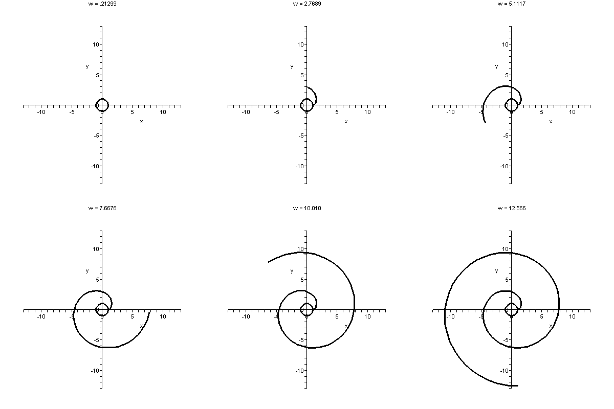
Finally to the right is an animated picture of the bug moving. Maybe you can understand this picture better: maybe (!!). This curve is more typical of parametric curves. I don't know any easy way to "eliminate" mention of the parameter. This seems to be an authentically (!) complicated parametric curve, similar to many curves which arise in physical and geometric problems. It has an official name. It is called the evolute of the circle.

My favorite parametric curve
This is x(t)=1/(1+t²) and y(t)=t³-t. I tried to analyze this curve a bit differently from the other examples by separately considering the horizontal and vertical components.

The horizontal control
Here we consider x as a function of t. The function has even degree and is therefore symmetric: if (t,x) is on the curve, so it (-t,x). Actually, the function is relatively simple. Consider positive t. As t increases, x decreases, and since 1+t2-->∞ x-->0. So we get a picture as shown below. Since this represents the horizontal part of the motion described by this parametric curve, the result is this in the (x,y) plane: the point for large negative t starts close to the x-axis. Then as t increases, it slowly moves right. At its largest it is 1 unit to the right of the vertical axis. Then it slowly moves back towards the vertical axis again.
The vertical control
In this case, I'm considering the y-component of the moving point. I could think of this as the vertical control of some sort of scanning machine. The function has odd degree and is antisymmetric (if (t,y) is on the curve, then (-t,-y) is on the curve). It is a cubic polynomial with three real roots, at 1, -1, and 0. The graph is shown to the right. The curve in the (t,y) plane starts very low left, then up, then down, then up, way way up on the right. But this is a description of the vertical motion. Now what could we "see" in the (x,y) plane? The point starts way way down (this is large negative y!), moves up, bounces down, and then finally moves way way up.

Combining these two motions can be difficult to do but with practice you will find it easier. A part of the combined motion, the whole parametric curve, is shown to the right. Indeed, it is a curve with a self-intersection.

I don't know how to describe this curve accurately and efficiently without the parametric "apparatus". The self-intersection occurs when t=1 and t=-1 (that's where x=0 and y<1, as shown in the picture). The point at which this occurs is (0,1/2).

Calculus?
Finally, very late in the lecture, I attempted some calculus. Here's what I said.

Suppose we want to analyze what happens when the parameter changes just a little bit, from t to t+Δt. Well, the point starts at (f(t),g(t)). What can we say happens at t+Δt? Well, f(t+Δt)≈f(t)+f´(t)Δt. Why is this true? You can think of this either 151 style as linear approximation, or from our more sophisticated 152 approach, this is the constant and linear terms in the Taylor series for f(t). Similarly for g(t) we know g(t+Δt)≈g(t)+g´(t)Δt. Therefore the point in the interval [t,t+Δt] moves from (f(t),g(t)) to (approximately!) (f(t)+f´(t)Δt,g(t)+g´(t)Δt). What is the slope of the line segment connecting these points?

Slope
Take the difference in second coordinates divided by the difference in the first coordinates. The result (there is a lot of cancellation) is g´(t)/f´(t). If this were an xy curve, this would be noted as dy/dx, the slope of the tangent line. In fact, people usually remember the result in the following way:

dy   dy/dt
-- = -----
dx   dx/dt

Speed
Since Distance=Rate·Time, and in the time interval [t,t+Δt] we move from (f(t),g(t)) to (approximately!) (f(t)+f´(t)Δt,g(t)+g´(t)Δt), we can get the speed (the Rate) by taking the distance between these points and dividing by Δt. There is more cancellation here, and the result is Speed=sqrt(f´(t)²+g´(t)²) or

         ___________
        /(dx)2 (dy)2   
Speed= / (--)+ (--) 
      /  (dt)  (dt) 

Please: I will show you a few simple examples of this Wednesday, and then go on to Polar Coordinates.

QotD
(More or less!) What is the state bird of New Jersey? I will report on the answers soon. Next time we will hand out (sigh) student evaluations. Come and write.

                                 SENATE, No. 241
                               STATE OF NEW JERSEY
                                    --------
                           Introduced January 29, 1935
                                  By Mr. KUSER
                 Referred to Committee on Miscellaneous Business
                    An Act to create a New Jersey State Bird
          BE IT ENACTED by the Senate and General Assembly of the State of
     New Jersey:
          1. The Eastern Goldfinch is hereby designated as the New Jersey
     State bird.
          2. This act shall take effect immediately.
                                    STATEMENT
          The purpose of this act is to create a State bird.  Forty-four
     of the States have already designated State birds.

What we know about Taylor (o.k., Maclaurin) series so far

• e^x=1+x+{x²/2}+{x³/6+...=∑_n=0^∞[xⁿ/n!] valid for all x.
• sin(x)=x-[x³/3!]+[x⁵/5!]-[x⁷/7!]+[x⁹/9!]...=∑_n=0^∞(-1)ⁿ⁺¹x²ⁿ⁺²/(2n+1)! valid for all x.
• cos(x)=1-[x²/2!]+[x⁴/4!]-[x⁶/6!]+[x⁸/8!]-[x¹⁰/10!]...=∑_n=0^∞(-1)ⁿ⁺¹x²ⁿ/(2n)! valid for all x.
• 1/(1-x)=1+x+x²+x³+...=∑_n=0^∞xⁿ valid for |x|<1.
• ln(1+x)=x-[x²/2]+[x³/3]-[x⁴/4]+[x⁵/5]+...=∑_n=1^∞[(-1)ⁿ⁺¹xⁿ/n] valid for |x|<1.

arctan
Let me try to find a Taylor series centered at 0 (a Maclaurin series) for arctan. Well, the general Maclaurin series is ∑_n=0^∞[f⁽ⁿ⁾(0)/n!]xⁿ so we can just try to compute some derivatives and evaluate them at 0. Let's see:
n=0 f(x)=arctan(x) so f(0)=arctan(0)=0.
n=1 f´(x)=1/(1+x²) so f´(0)=Stop this right now! Why? Because this way is madness. Here is the 7^th derivative of arctan(x):

              6       4       2
720 (7 x  - 35 x  + 21 x  - 1)
------------------------------
              2 7
        (1 + x )

Instead look at

 1
----
1+x2

• arctan(x)=x-[x³/3]+[x⁵/5]-[x⁷/7]+[x⁹/9]...= ∑_n=0^∞[(-1)²ⁿ⁺¹x²ⁿ⁺¹/(2n+1)]

Computing π
This series has been used to compute decimal approximations of π. For example, if x=1, arctan(1)=π/4, so this must be 1-1/3+1/5-1/7+... but the series converges very slowly (for example, the 1000^th partial sum multiplied by 4 gives the approximation 3.1406 for π which is not so good for all that arithmetic!) . Here is a history of some of the classical efforts to compute decimal digits of π. You can search some of the known decimal digits of π here. There are more than a trillion (I think that is 10¹²) digits of π's decimal expansion known. Onward! The methods used for such computations are much more elaborate than what we have discussed.

Binomial series with m=1/3
One of Newton's most acclaimed accomplishments was the description of the Maclaurin series for (1+x)^m. Here is more information. In class and here, I'll specialize by analyzing what happens when m=1/3. We'll use a direct approach by taking lots of derivatives and trying to understand ∑_n=0^∞[f⁽ⁿ⁾(0)/n!]xⁿ.

• n=0 f(x)=(1+x)^1/3 so that f(0)=(1+0)^1/3=1.
• n=1 f´(x)=(1/3)(1+x)^-2/3 so that f´(0)=(1/3)(1+0)^-2/3=(1/3).
• n=2 f´´(x)=(1/3)(-2/3)(1+x)^-5/3 so that f´´(0)=(1/3)(-2/3)(1+0)^-5/3=(1/3)(-2/3).
• n=3 f⁽³⁾(x)=(1/3)(-2/3)(-5/3)(1+x)^-8/3 so that f⁽³⁾(0)=(1/3)(-2/3)(-5/3)(1+0)^-8/3=(1/3)(-2/3)(-5/3).
• n=3 f⁽⁴⁾(x)=(1/3)(-2/3)(-5/3)(-8/3)(1+x)^-11/3 so that f⁽⁴⁾(0)=(1/3)(-2/3)(-5/3)(-8/3)(1+0)^-11/3=(1/3)(-2/3)(-5/3)(-8/3).

Naive numerical use
So you want to compute (1.05)^1/3? This is a doubtful assumption, and anyway wouldn't you do a few button pushes on a calculator? But let's see:
Suppose we use the first two terms of the series and let x=.05:
     (1+.05)^1/3=1+(1/3)(.05)+Error
What's interesting to me is how big the Error is. Of course, we have the Error Bound, which states that |Error|≤[K/(n+1)!]|x-a|ⁿ⁺¹. Here, since the top term in the approximation is the linear term, we have n=1. And a, the center of the series, is 0, and x, where we are approximating, is .05. Fine, but the most complicated part still needs some work. K is an overestimate of the absolute value of the second derivative of f on the interval connecting 0 and .05. Well (look above!) we know that f⁽²⁾(x)=(1/3)(-2/3)(1+x)^-5/3. We strip away the signs (not the sign in the exponent, since that means something else!). We'd like some estimate of the size of (2/9)(1+x)^-5/3 on [0,.05]. Well, it is exactly because of the minus sign in the exponent that we decide the second derivative is decreasing on the interval [0,.05] and therefore the largest value will be at the left-hand endpoint, where x=0. So plug in 0 and get 1/9(1+0)^-5/3=2/9. This is our K. So the Error Bound gives us [(2/9)/2!](.05)², which is about .00027. We have three (and a half!) decimal digits of accuracy in the simple 1+(1/3)(.05) estimate.

What if we wanted to improve this estimate? Well, we can try another term. By this I mean use 1+(1/3)(.05)+[(1/3)(-2/3)/2](.05)² as an estimate of (1.05)^1/3. How good is this estimate? Again, we use the Error Bound: |Error|≤[K/(n+1)!]|x-a|ⁿ⁺¹. Now n=2 and a=0 and x=.05, and K comes from considering f⁽³⁾(x)=(1/3)(-2/3)(-5/3)(1+x)^-8/3. We need to look at (10/27)(1+x)^-8/3 on [0,.05]. The exponent is again negative (what an accident not -- these methods are actually used and things should be fairly simple!) and therefore the function is again decreasing and an overestimate is gotten by looking at the value when x=0, so (10/27)(1+x)^-8/3 becomes (10/27)(1+0)^-8/3=(10/27). Hey, [K/(n+1)!]|x-a|ⁿ⁺¹ in turn becomes [(10/27)/3!](.05)³, about .000008, even better.

Approximating a function on an interval
People usually use the partial sums considered above in a more sophisticated way. For example, consider replacing (1+x)^1/3 by T₂(x)=1+(1/3)x+[(1/3)(-2/3)/2!]x²=1+(x/3)-(x²/9) anywhere on the interval [0,.05]. I like polynomials, because they can be computed just by adding and multiplying. The function (1+x)^1/3 has this irritating and weird exponent, that I, at least, can't readily estimate. What about the error? The Error Bound declares that an overestimate of the error is [K/3!]|x-0|³. Now if 0<x<.05, then the largest x³ can be is (.05)³. What about K? Again, we look at the third derivative with the signs (not the exponent sign!) dropped. This is (10/27)(1+x)^-8/3 which we are supposed to estimate for any x in [0,.05]. But since the third derivative is still decreasing (-1/3<0) again the K is gotten by plugging in x=0. 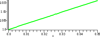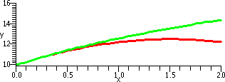Hey: the estimate is the same as what we had before, about .000008. Below are some pictures illustrating what's going on.

(1+x)1/3 & T2(x) on [0,.05]	(1+x)1/3 & T2(x) on [0,2]
Comments Yes, there really really are two curves here. One, (1+x)1/3, is green and one, T2(x)=1+(x/3)-(x2/9), is red. But the pixels in the image overlay each other a lot, because the error, .000008, makes the graphs coincide on the [0,.05] interval. There are only a finite number of positions which can be colored, after all!	Comments This graph perhaps shows more about what's going on. The domain interval has been changed to [0,2]. The K in the Error Estimate is not changed, but the x's now range up to 2. So [K/3!]x3 becomes as a worst case estimate [(10/27)/3!]23, which is about .49. You can see T2(x) revealed (!) as just a parabola opening downward (hey, 1+(x/3)-(x2/9) has –1/9 as x2 coefficient!). The two curves are close near x=0, and then begin to separate as x grows larger.

Improving the approximation
The whole idea is maybe by increasing the partial sum (going to T_n(x)'s with higher n's) we will get better approximations. This is only usable if the approximations are easy to compute (nice polynomials with simple coefficients) and if the error estimates are fairly easy to do. This actually occurs so that people use these ideas every day.

Binomial series in general
Suppose m is any number (yes: any number). Then

• (1+x)^m=1+mx+[m(m-1)/1·2]x²+[m(m-1)(m-2)/1·2·3]x³+[m(m-1)(m-2)(m-3)/1·2·3·4]x⁴+..., valid for |x|<1.

How to gamble
I gave a wonderful and colorful presentation about how to gamble. Well, I introduced certain basic language and ideas. It ain't clear how wonderful and effective the presentation was -- students may have some ideas. Even if you are not interested in gambling, the same ideas and computations are used to investigate real situations like the average life span of computer components or stressed objects in structures or ... lots of things. Here are some notes I wrote last year for a 152 class on this material.

The list ...

• e^x=1+x+{x²/2}+{x³/6+...=∑_n=0^∞[xⁿ/n!] valid for all x.
• sin(x)=x-[x³/3!]+[x⁵/5!]-[x⁷/7!]+[x⁹/9!]...=∑_n=0^∞(-1)ⁿ⁺¹x²ⁿ⁺²/(2n+1)! valid for all x.
• cos(x)=1-[x²/2!]+[x⁴/4!]-[x⁶/6!]+[x⁸/8!]-[x¹⁰/10!]...=∑_n=0^∞(-1)ⁿ⁺¹x²ⁿ/(2n)! valid for all x.
• 1/(1-x)=1+x+x²+x³+...=∑_n=0^∞xⁿ valid for |x|<1.
• ln(1+x)=x-[x²/2]+[x³/3]-[x⁴/4]+[x⁵/5]+...=∑_n=1^∞[(-1)ⁿ⁺¹xⁿ/n] valid for |x|<1.
• arctan(x)=x-[x³/3]+[x⁵/5]-[x⁷/7]+[x⁹/9]...= ∑_n=0^∞[(-1)²ⁿ⁺¹x²ⁿ⁺¹/(2n+1)]
• (1+x)^m=1+mx+[m(m-1)/1·2]x²+[m(m-1)(m-2)/1·2·3]x³+[m(m-1)(m-2)(m-3)/1·2·3·4]x⁴+..., valid for |x|<1.

Item 1 Please compute (3²+4²)^1/2. Since 3²=9 and 4²=16, their sum is 25 which has square root 5. The sum of 3 and 4 is 7. Notice that 5≠7. Therefore (3²+4²)^1/2 and 3+4 are not equal. No amount of algebraic effort should be spent trying to massage one into the other! Please!!!

Item 2 Consider the function 2^x. Its graph looks like this: 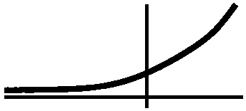and so the slopes of all of the lines tangent to the graph are positive -- they are all tilted up. Now consider x2^x-1. I think that when x=0 this function is 0. So there is no way that the derivative of 2^x can be x2^x-1! Please!!!
What is the derivative of 2^x? Since 2^x=(e^ln(2))^x=e^{ln(2)}x (repeated exponentiations multiply!) we can differentiate using the Chain Rule:
    d/dx[e^{ln(2)}x]=e^{ln(2)}x(ln(2))=2^xln(2).
So the derivative of 2^x is 2^xln(2).
And the derivative of 17^x is 17^xln(17).
And the derivative of (1/134)^x is (1/134)^xln(1/134).
And the derivative of π^x is π^xln(π).
ETC.

Background
So far we've learned that partial sums of Taylor series are Taylor polynomials. And by using the Error Bound for Taylor polynomials, we see that some Taylor series converge, and they converge to the functions which "created" them. Since a function has only one power series centered at each point, and since power series can be added, multiplied, divided, differentiated, integrated, and even more, well, anything you do (if it is correct!) to a power series gets a new power series, valid inside its radius of convergence.

So far
Our Error Bound analysis has given us these:

• e^x=1+x+{x²/2}+{x³/6+...=∑_n=0^∞[xⁿ/n!] valid for all x.
• sin(x)=x-[x³/3!]+[x⁵/5!]-[x⁷/7!]+[x⁹/9!]...=∑_n=0^∞(-1)ⁿ⁺¹x²ⁿ⁺²/(2n+1)! valid for all x.
• cos(x)=1-[x²/2!]+[x⁴/4!]-[x⁶/6!]+[x⁸/8!]-[x¹⁰/10!]...=∑_n=0^∞(-1)ⁿ⁺¹x²ⁿ/(2n)! valid for all x.

Book problem: 10.7, #21
Use multiplication to find the first four terms in the Maclaurin series for e^xsin(x).
You may, if you wish, start finding derivatives, evaluating them at 0, and plug into the formula ∑_n=0^∞[f⁽ⁿ⁾(0)/n!]xⁿ. I don't want to because I would prefer to be LAZY. If asked to contribute to the design of a car, would you first invent the wheel? Well, maybe, if you could really conceive of a better wheel. The idea is to take advantage of what's already done. Please!
e^xsin(x)=(1+x+{x²/2}+{x³/6}+...)(x-[x³/3!]+[x⁵/5!]...)=
    (multiplying by 1)(x-[x³/6]+[x⁵/120])+
    (multiplying by x)(x²-[x⁴/6]+[x⁶/24])+
    (multiplying by x²/2)([x³/2]-[x⁵/12]+[x⁷/48])+
    (multiplying by x³/6)([x⁴/6]-[x⁶/36]+[x⁸/144])+
    (multiplying by x⁴/24)([x⁵/24]-[x⁷/stuff]+[x⁹/more stuff])+
Now I'll collect terms, going up by degrees:
x+x²-[x³/6]+[x³/2]-[x⁴/6] +[x⁴/6]]+[x⁵/120]-[x⁵/12]+[x⁵/24] Stop! since I only need the "bottom" 4 (in degree). I did go on, past the x⁴ terms, since I noticed they canceled. I interpreted the problem as asking for the first 4 non-zero terms.
The hard computation is [x⁵/120]-[x⁵/12]+[x⁵/24]. But 1/120-1/12+1/24=1/120-10/120+5/120=-4/120=-1/30. My answer is therefore
x+x²+[x³/3]-[x⁵/30].

Book problem: 10.7, #14
Find the Maclaurin series of cos(sqrt(x)). Since cos(x)=1-[x²/2!]+[x⁴/4!]-[x⁶/6!]+[x⁸/8!]-[x¹⁰/10!]...=∑_n=0^∞(-1)ⁿ⁺¹x²ⁿ/(2n)! I know that cos(sqrt(x))=1-[(sqrt(x))²/2!]+[(sqrt(x))⁴/4!]-[(sqrt(x))⁶/6!]+[(sqrt(x))⁸/8!]-[(sqrt(x))¹⁰/10!]...=∑_n=0^∞(-1)ⁿ⁺¹(sqrt(x))²ⁿ/(2n)! and so cos(sqrt(x))=1-[x/2!]+[x²/4!]-[x³/6!]+[x⁴/8!]-[x⁵/10!]...=∑_n=0^∞(-1)ⁿ⁺¹xⁿ/(2n)!, and please be LAZY.

Book problem: 10.7, #19
Find the Maclaurin series of (1-cos(x²)/x. Since cos(x)=1-[x²/2!]+[x⁴/4!]-[x⁶/6!]+... I know that cos(x²)=1-[x⁴/2!]+[x⁸/4!]-[x¹²/6!]+... and 1-cos(x²)=[x⁴/2!]-[x⁸/4!]+[x¹²/6!]+... so that (1-cos(x²)/x=[x³/2!]-[x⁷/4!]+[x¹¹/6!]+...

An integral
Consider ∫₀^.84cos(x³dx. I don't know how to do this with FTC. That is, I can't find an antiderivative of cos(x³) in terms of "familiar" functions. But what if you really needed to know the value of this integral (hey, it's .81925 to 5 decimal place accuracy). We could use the Trapezoid Rule or Simpson's Rule or ... Let me show you another way. Learning new tricks is good, because sometimes the old tricks won't work so easily.

Since cos(x)=1-[x²/2!]+[x⁴/4!]-[x⁶/6!]+[x⁸/8!]... I know that cos(x³)=1-[x⁶/2!]+[x¹²/4!]-[x¹⁸/6!]+[x²⁴/8!]... and we can find the antiderivative:
∫cos(x³)dx=∫1-[x⁶/2!]+[x¹²/4!]-[x¹⁸/6!]+[x²⁴/8!]...dx=x-[x⁷/7·2]+[x¹³/(13·24)]-[x¹⁹/(19·720]+... and now we evaluate |₀^.84 so the value of the integral is .84-[.84⁷/7·2]+[.84¹³/(13·24)]-[.84¹⁹/(19·720]+...

This is ugly, but you should notice that it satisfies the Alternating Series Test: the terms alternate in sign, their magnitudes decrease, and the limit is 0. Therefore a partial sum is as accurate as the first omitted term (that is emphatically not generally true for all series!).

We computed [.84¹⁹/(19·720] and it was about .000002. So the integral, to 5 decimal place accuracy, is .84-[.84⁷/7·2]+[.84¹³/(13·24)]. And we computed this, and we got the predicted value, .81925.

Moral lesson?
Not clear to me there is a great moral lesson in this, but it is a neat way, with not much work, to compute this particular integral. One could even imagine doing this by hand if necessary (not really much arithmetic). I would rather not compute a Trapezoid or Simpson's Rule approximation by hand.

Logarithm
What the Maclaurin series of ln(x)? This is a trick question because y=ln(x) looks like this and the limit of ln(x) as x-->0⁺ is -∞ so ln(x) can't have a Taylor series centered at 0. What's a good place to consider? Since ln(1)=0, we could center the series at 1. Most people would still like to compute near 0, though, so usually the function is moved instead! That is, consider ln(1+x) whose graph now behaves nicely at 0 so we can analyze it there.

If f(x)=ln(1+x), I want to "find" ∑_n=0^&infin[f⁽ⁿ⁾(0)/n!]xⁿ. Well, f(0)=ln(1+0)=ln(1)=0, so we know the first term. Now f´(x)=1/(1+x) so that ... wait, wait: remember to try to be LAZY.

Look at

 1
---
1+x

Computing with ln
What if x=-1/2 in the previous equation? Then ln(1-1/2)=ln(1/2)=-ln(2) and this is approximately -69314. A friend of mine has just computed &sum_n=1¹⁰[(-1)ⁿ⁺¹(-.5)ⁿ/n] and this turns out to be -.69306. We only get 3 decimal places of accuracy. It turns out that this series converges relatively slowly compared to the others we've already seen, which have the advantage of factorials in the denominator. So this series is usually not directly used for numerical computation, but other series related to it are used.

Book problem: 10.7, #9
Find the Maclaurin series of ln(1-x²).
Be LAZY. We know that
ln(1+x)=x-[x²/2]+[x³/3]-[x⁴/4]+[x⁵/5]+...=&sum_n=1^∞[(-1)ⁿ⁺¹xⁿ/n]. This
so we can substitute -x² for x and get
ln(1-x²)=-x²-[(-x²)²/2]+[(-x²)³/3]-[(-x²)⁴/4]+[(-x²)⁵/5]+...=&sum_n=1^∞[(-1)ⁿ⁺¹(-x²)ⁿ/n] and further
ln(1-x²)=-x²-[x⁴/2]-[x⁶/3]-[x⁸/4]-[x¹⁰/5]+...=-&sum_n=1^∞[(-1)ⁿ⁺¹x²ⁿ/n] (valid for |x|<1).

Computing a value of a derivative
I know that the degree 8 term in the Maclaurin series for ln(1-x²) is -[x⁸/4]. But it is also supposed to be (by abstract "theory") [f⁽⁸⁾(0)/8!]x⁸. This means "clearly" (!!!) that -1/4=[f⁽⁸⁾(0)/8!] and therefore f⁽⁸⁾(0)=-8!/4.

That's if you desperately wanted to know the value of the derivative. An alternate strategy would be to compute the 8^th derivative and evaluate it at x=0. Here is that derivative:

             6    8       4       
  10080 (28 x  + x  + 70 x  + 28 x  + 1)
- --------------------------------------
                   2 8
            (-1 + x )

Second exams returned ...
The second exams were returned. Here is a version of that exam. An answer sheet was also distributed, and information about the grades and grading is available. Please let me know if you have questions about the grading after you read the answer sheet and the grading guide.

Definition A power series centered at x0 (a fixed number) is an infinite series of the form ∑n=0∞cnxn where the x is a variable and the cn are some collection of coefficients. It is sort of like an infinite degree polynomial. Usually I (and most people) like to take x0 to be 0 because this just makes thinking easier.

Calculus and power series Hypothesis Suppose the power series ∑n=0∞an (x-x0)n has some positive radius of convergence, R, and suppose that f(x) is the sum of this series inside its radius of convergence. Differentiation The series ∑n=0∞n an (x-x0)n-1 has radius of convergence R, and for the x's where that series converges, the function f(x) can be differentiated, and f´(x) is equal to the sum of that series. Integration The series ∑n=0∞[an/(n+1)] (x-x0)n+1 has radius of convergence R, and for the x's where that series converges, the sum of that series is equal to an indefinite integral of f(x), that is ∫f(x)dx.

Convergence and divergence A power series centered at x0 always has an interval of convergence with the center of that interval equal to x0. Inside the interval of convergence, the power series converges absolutely and therefore converges. Outside the interval, the power series diverges. The power series may or may not converge on the boundary of the interval. The interval may have any length between 0 and ∞. Half the length of the interval is called the radius of convergence.

If a function has a power series then ...
Suppose I know that f(x) is equal to a sum like A+B(x-x₀)+C(x-x₀)²+D(x-x₀)³+E(x-x₀)⁴+... and I would like to understand how the coefficients A and B and C and D etc. relate to f(x). Here is what we can do.

Step 0 Since f(x)=A+B(x-x₀)+C(x-x₀)²+D(x-x₀)³+E(x-x₀)⁴+... if we change x to x₀ we get f(x₀)=A. All the other terms, which have powers of x-x₀, are 0.
Step 1a Differentiate (or, as I said in class, d/dx) the previous equation which has x's, not x₀'s. Then we have f´(x)=0+B+2C(x-x₀)¹+3D(x-x₀)²+4E(x-x₀)³+...
Step 1b Plug in x₀ for x and get f´(x₀)=B. All the other terms, which have powers of x-x₀, are 0.
Step 2a Differentiate (or, as I said in class, d/dx) the previous equation which has x's, not x₀'s. Then we have f´´(x)=0+0+2C+3·2D(x-x₀)¹+4·3E(x-x₀)²+...
Step 2b Plug in x₀ for x and get f´´(x₀)=2C, so C=[1/2!]f⁽²⁾(x₀). All the other terms, which have powers of x-x₀, are 0.
Step 3a Differentiate (or, as I said in class, d/dx) the previous equation which has x's, not x₀'s. Then we have f⁽³⁾(x)=0+0+0+3·2·1D+4·3·2E(x-x₀)¹+...
Step 3b Plug in x₀ for x and get f⁽³⁾)(x₀)=3·2··1D=3!C so D=[1/3!]f⁽³⁾(x₀). All the other terms, which have powers of x-x₀, are 0.
ETC. Continue as long as you like. What we get is the following fact: if f(x)=∑_n=0^∞a_n(x-x₀)ⁿ then a_n=[f⁽ⁿ⁾(x₀)/n!]. This is valid for all non-negative integers, n. Actually, this formula is one of the reasons that 0! is 1 and the zeroth derivative of f is f itself. With these understandings, the formula works for n=0.
What this means is that
If a function is equal to a power series, that power series must be the Taylor series of the function.
I hope you notice, please please please, that the partial sums of the Taylor series are just the Taylor polynomials, which we studied earlier.

Usually I'll take x₀=0, as I mentioned. Then the textbook and some other sources call the series the Maclaurin series. A useful consequence of this result (it will seem sort of silly!) is that if a function has a power series expansion, then it has exactly one power series expansion (because any two such series expansions are both equal to the Taylor series, so they must be equal). This means if we can get a series expansion using any sort of tricks, then that series expansion is the "correct one" -- there is only one series expansion. I'll show you some tricks, but in this class I think I will just try some standard examples which will work relatively easily.

e^x
I'll take x₀=0. Then all of the derivatives of e^x are e^x, and the values of these at 0 are all 1. So the coefficients of the Taylor series, a_n, are [f⁽ⁿ⁾(x₀)/n!]=1/n!. The Taylor series for e^x is therefore ∑_n=0^∞[1/n!]xⁿ.

e^-.3
Let's consider the Taylor series for e^x when x=-.3. This is ∑_n=0^∞[1/n!](-.3)ⁿ. What can I tell you about this? Well, for example, my "pal" could compute a partial sum, say ∑_n=0¹⁰[1/n!](-.3)ⁿ. The result is 0.7408182206. That's nice. But what else do we know? Well, this partial sum is T₁₀(-.3), the tenth Taylor polynomial for e^x centered at x₀=0, and evaluated at -.3. The Error Bound gives an estimation of | T₁₀(-.3)-e^-.3|. This Error Bound asserts that this difference is at most [K|-.3-0|¹¹/11!], where K is some overestimate of the 11^th derivative of e^x on the interval between -.3 and 0. Well, that 11^th derivative is also e^x. And we know that e^x is increasing (exponential growth after all!) so that for x's in the interval [-.3,0], e^x is at most e⁰=1, and we can take that for K. So the Error Bound is 1|-.3-0|¹¹/11!. Now let's look at some numbers:
|-.3|¹¹=0.00000177147 and 11!=39,916,800, and their quotient is about 4·10^-14.
This means that e^-.3 and T₁₀(-.3) agree at least to 13 decimal places. Indeed, to 10 decimal places, e^-.3 is reported as 0.7408182206, the same number we had before. Wow? Wow!

Let's change 10 to n and 11 to n+1. Then |T_n(-.3)-e^-.3| is bounded by K|-.3-0|ⁿ⁺¹/(n+1)!. Here K=1 again because all of the derivatives are the same, e^x. Since 1|-.3-0|ⁿ⁺¹/(n+1)!-->0 as n-->∞ what do we know?

I think that the sequence {T_n(-.3)} converges, and its limit is e^-.3. Since this sequence of Taylor polynomial values is also the sequence of partial sums of the series ∑_n=0^∞[1/n!](-.3)ⁿ, I think that the series converges, and its sum is e^-.3. Therefore
e^-.3=∑_n=0^∞[1/n!](-.3)ⁿ.

e^.7
We tried the same thing when x=.7 and by the same thing, I think we first examined T₁₀(.7). This is ∑_n=0¹⁰[1/n!](.7)ⁿ. To 10 decimal places, this is 2.0137527069. We have information from the Error Bound. It declares that |T₁₀(.7)-e^.7| is no larger than K|.7-0|¹¹/11!. Here K is an overestimate of the 11^th derivative, which is e^x, on the interval [0,.7]. The exponential function is (still!) increasing, so the largest value is at x=.7. But I don't know e^.7. I do know it is less than e¹ which I hardly know also. I will guess that e<3. So a nice simple K to take is 3. Let me try that. The Error Bound is less than 3|.7-0|¹¹/11!. Let's do the numbers here.
11!=39,916,800 (again) but .7¹¹=0.0197732674 (small, but not as small as |-.3|¹¹). The Error Bound 3|.7-0|¹¹/11! is about 2·10^-9, not quite as small.
Now e^.7, to 10 decimal places, is 2.0137527074 and this is close enough to the sum value quoted before.

Again, go to n and n+1: |T_n(.7)-e^.7| is less than 3|.7-0|ⁿ⁺¹/(n+1)!, and again, as n-->∞ this goes to 0. Our conclusion is:
The sequence {T_n(.7)} converges, and its limit is e^.7. Since this sequence of Taylor polynomial values is also the sequence of partial sums of the series ∑_n=0^∞[1/n!](.7)ⁿ, I think that the series converges, and its sum is e^.7. Therefore
e^.7=∑_n=0^∞[1/n!](.7)ⁿ.

e⁵⁰
Just one more example partly because we'll see some strange numbers. Let's look at T₁₀(50) which is ∑_n=0¹⁰[1/n!]50ⁿ. This turns out to be (approximately!) 33,442,143,496.7672, a big number. The Error Bound says that |T₁₀(50)-e⁵⁰| is less than K|50-0|¹¹/11! where K is the largest e^x can be on [0,50]. That largest number is e⁵⁰ because e^x is increasing. I guess e⁵⁰ is less than, say, 3⁵⁰, which is about 7·10²³. I'll take that for K. Now how big is that Error?
K|50-0|¹¹/11! still has 11! underneath but now the top is growing also. This is approximately 9·10³⁴, a sort of big number.

The situation for x=50 may look hopeless, but it isn't really. To analyze |T_n(50)-e⁵⁰| we need to look at K[(50)ⁿ⁺¹/(n+1)!]. Here the fraction has power growth on the top and factorial growth on the bottom. Well, we considered this before. I called it a "rather sophisticated example". Factorial growth is faster eventually than power growth. So this sequence will -->0 as n-->∞. A similar conclusion occurs:
e⁵⁰=∑_n=0^∞[1/n!](50)ⁿ.

In fact, e⁵⁰ is 5.18470552858707·10²¹ while the partial sum with n=100, ∑_n=0¹⁰⁰[1/n!](50)ⁿ has value 5.18470552777323·10²¹: the agreement is not too bad, relatively.

And generally for exp ...
It turns out that ∑_n=0^∞[1/n!]xⁿ converges for all x and its sum is always e^x. The way to verify this is what we just discussed. Most actual computation of values of the exponential function relies on partial sums of this series. There are lots of computational tricks to speed things up, but the heart of the matter is the Taylor series for the exponential function.

cosine
We analyzed cosine's Taylor polynomials, taking advantage of the cyclic (repetitive) nature of the derivatives of cosine: cosine-->-sine-->-cosine-->sine then back to cosine. At x=0, this gets us a cycle of numbers: 1-->0-->-1-->0. The Taylor series for cosine centered at 0 leads off like this:
1-[x²/2!]+[x⁴/4!]-[x⁶/6!]+[x⁸/8!]-[x¹⁰/10!]...

It alternates in sign, it has only terms of even degree, and each term has the reciprocal of an "appropriate" factorial (same as the degree) as the size of its coefficient.

cos(1/3)
How close is 1-[(1/3)²/2!]+[(1/3)⁴/4!]-[(1/3)⁶/6!]+[(1/3)⁸/8!]-[(1/3)¹⁰/10!] to cos(1/3)? Here we sort of have two candidates because T₁₀(1/3) is the same as T₁₁(1/3) since the 11^th degree term is 0.
Error bound, n=10 So we have K|(1/3)-0|¹¹/11!, where K is a bound on the size of the 11^th derivative of cosine. Hey: I don't care much in this example, because I know that this derivative is +/-cosine or +/-sine, so that I can take K to be 1. Now it turns out that (1/3)¹¹/11! is about 1.4·10^-14. This is tiny, but ...
Error bound, n=11 This is even better. So we have K|(1/3)-0|¹²/12!, where K can again be taken as 1 (this is easier than exp!) So (1/3)¹²/12! is about 4·10^-15, even tinier.

Hey, cos(1/3)=0.944956946314738 and T₁₀(1/3)=0.944956946314734.

cosine and sine estimates
For both cosine and sine, the estimates are easy because K for both can be taken to be 1. And the results are that the appropriate Taylor series for both functions converge to the function values. That is:
cos(x)=∑_n=0^∞(-1)ⁿ⁺¹x²ⁿ/(2n)! for all x. The first few terms look like 1-[x²/2!]+[x⁴/4!]-[x⁶/6!]+[x⁸/8!]-[x¹⁰/10!]...
sin(x)=∑_n=0^∞(-1)ⁿ⁺¹x²ⁿ⁺²/(2n+1)! for all x. The first few terms look like x-[x³/3!]+[x⁵/5!]-[x⁷/7!]+[x⁹/9!]...

A series for cos(x³)
We can use the series we know to "bootstrap" and get other series. That is, we build on known results. For example, since we know that cos(x)=1-[x²/2!]+[x⁴/4!]-[x⁶/6!]+[x⁸/8!]-[x¹⁰/10!]... for all x, I bet cos(x³)=1-[(x³)²/2!]+[(x³)⁴/4!]-[(x³)⁶/6!]+[(x³)⁸/8!]-[(x³)¹⁰/10!]... which is 1-[x⁶/2!]+[x¹²/4!]-[x¹⁸/6!]+[x²⁴/8!]-[x³⁰/10!]... and this is much easier than trying to compute derivatives of cos(x³) which we would have to do to plug in the values of the derivatives in the Taylor series. The Chain Rule makes things horrible. For example, the fifth derivative of cos(x³) is -243sin(x³)x¹⁰+1620cos(x³)x⁷+2160sin(x³)x⁴-360cos(x³)x and that's fairly horrible.

How about x²cos(x³)?
Multiply the previous series by x². The result is x²cos(x³)=x²-[x⁸/2!]+[x¹⁴/4!]-[x²⁰/6!]+[x²⁶/8!]-[x³²/10!]... Wow?

QotD
What are the first four non-zero terms of the Taylor series for x³e^-2x centered at 0?
Since e^x=1+x+x²/2+x³/6+... (3! is 6) we know e^-2x=1-2x+(-2x)²/2+(-2x)³/6+...=1-2x+4x²/2-8x³/6+...= =1-2x+2x²-4x³/3+... and then we multiply by x³. The answer is x³-2x⁴+2x⁵-4x⁶/3.

Maintained by greenfie@math.rutgers.edu and last modified 4/14/2008.