| Wednesday, November 15 | (Lecture 19) |
|---|
Another problem
f´´(x)=5x2+11/x2
f´(1)=3
f(1)=7
And another ...
f´´(x)=3cos(4x)+8sin(x)
f´(5Pi)=3
f(4Pi)=-7
And another ...
Just first order this time:
f´(x)=sqrt(1+x3)
f(0)=2
Can't antidifferentiate in terms of familiar functions, so ... a
qualitative study.
Just one more
f´(x)=x/(1+x3)
f(2)=3
Vocabulary
Direction field; solution curve
An actual solution can be written ...
Numbers?
f´(x)=sqrt(1+x3)
f(0)=2
How can we get f(1), then?
| Monday, November 13 | (Lecture 18) |
|---|
Problem #2
General facts
Yet another problem
| Wednesday, November 8 | (Lecture 18) |
|---|
Second attempt (zooming in)
(Bumps)
More zooming
(Wiggles)
The whole thing
Moving on: a max/min problem
| Monday, November 6 | (Lecture 18) |
|---|
The Consumer Price Index
I wrote the changes in the consumer price index during three periods
of U.S. history, and tried to explain how these numbers, reflecting
data which was gathered by looking at prices, implied information
about the shape of the CPI over time. In particular, these shapes
showed that the CPI increased and decreased, and that the
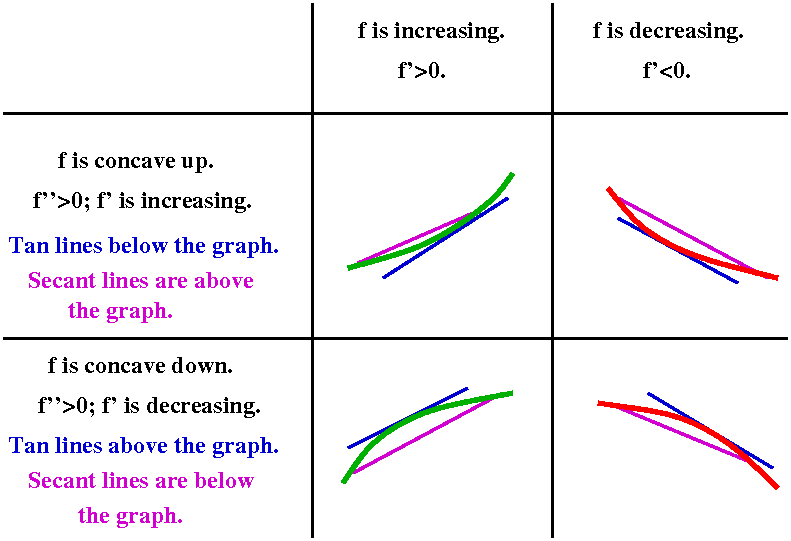
CPI graph also "curved". This curving is called concavity. Logically
the concavity and the {in|de}creasing nature of the curve are not
connected. I tried to show this in the diagram below.
Concavity and {In|de}creasing

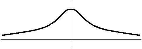 Graphing e-x2
I asked students to have and
use a graphing calculator. The result was sort of like what is shown
to the right. Realize that looking at the graph is not "cheating" and
I use graphing software whenever possible. At the same time, the
graphing software can be fooled -- deceptive results can occur,
and sometimes you need to look really closely at the calculus side of
things.
If f(x)=e-x2 then f'(x)=(e-x2)(-2x). The exponential function is very nice. It is never 0 and always positive. Therefore the only x for which f'(x)=0 is when -2x=0. So x=0 is the only critical number. Now reasoning using the Intermediate Value Theorem says that f (which is certainly continuous!) can have only one sign for x<0 and one sign for x>0 (or else f(x) would have to have to be 0 again). We can check signs at, say. x=1 and x=-1. f is increasing in (-infinity,0) and f is decreasing in (0,infinity). Naturally 0 represents a local (and indeed, absolute!) maximum.
What information can we get from the second derivative? If we use the product and the chain rule correctly, then f''(x)=(e-x2)(4x2-2). Logic similar to the preceding asserts that this is 0 exactly when the non-exponential factor is 0. But 4x2-2=0 when x=+/-sqrt(2). Again, we can check signs in between the 0's of f'', and f will be concave up for x<-1/sqrt(2) and for x>1/sqrt(2). For x between -1/sqrt(2) and +1/sqrt(2), the graph will be concave down. The points where x=+/-1/sqrt(2) are where the concavity of f changes: these are called inflection points. These particular inflection points are related to the standard deviation, which represents dispersal from an average when this function is used in statistics.
Graphing a degree 3 polynomial from the book
I looked at y=2-15x+9x2-x3, which is problem #3
in section 4.5. This is a problem in the textbook. Again we began
with a graphing calculator result. We computed the first and second
derivatives and found out where the signs of these functions
changed. From this we were able to get information about increasing
and decreasing and inflection points.
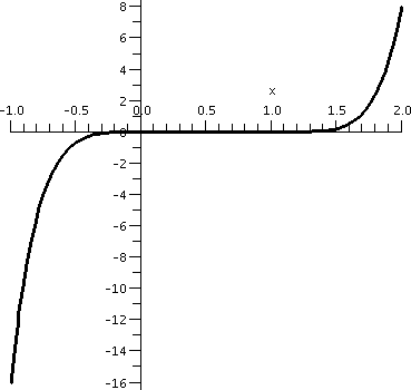 Graphing x3(x-1)4
Here I invited students again to use a graphing calculator and try to
see what y=x3(x-1)4 "looked like". I did remark
that the "action" took place somewhere between -1 and 2. The result of
this was something like the graph shown to the right. I believe that
calculators and graphing devices are wonderful, but sometimes they
almost conceal what's going on.
Here f(x)=x3(x-1)4. If we want to find out where
f is increasing and decreasing, we really should look at
f´(x). For this we need the product rule and the chain rule. So:
f´(x)=3x2(x-1)4+x34(x-1)3.
Generally I am against "simplifying" because I view it as mostly a
chance to make lots of mistakes. But here some simplifying will reveal
structure in the derivative. So please notice the common factors, and
what you get is as follows:
f´(x)=x2(x-1)3(3(x-1)+4x)=x2(x-1)3(7x-3).
What can we tell about where the derivative is 0 and where it is positive and where it is negative? Well, the different factors allow us to deduce that the derivative is 0 at x=0 and x=1 and x=3/7.
If x is very large positive, say, then f(x) is a product of three factors, all of which are positive. And if x is very large negative, then the x2 is positive and the (x-1)3 is negative and the 7x-3 is negative. Therefore f(x) in that range is positive also. So we have learned (using logic from the Intermediate Value Theorem as before) that the derivative is positive on at least the intervals (-infinity,0) and (1,infinity). There is a chance for the derivative to change signs at x=0, but the factor which controls sign change there is x2: since 2 is even, there is no sign change at x=0. But there is a sign change at x=3/7 and at x=1. So now we have broken up the real line into pieces
    Deriv is +     Still +          Now it is -        Back to + here
<---------------0-----------3/7--------------------1------------------->
 Func increases   increases     The func decreases   Here it decreases
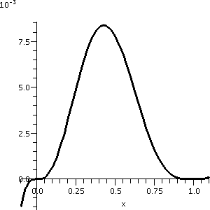 So from this I learn that f has critical points at 0 and 3/7 and 1. We
can also learn that f has a local max at 3/7 and a local min at
1. This is not entirely clear from the initial graph. Actually,
if we just look at the graph from -.1 to 1.1, you can see some of the
structure. This is shown to the right. Please notice that the vertical
scale of this graph is very small. This might all be difficult to see
without looking at the calculus first.
Then we considered the concavity of this function, and made some
guesses about the number and location of inflection points. We can be
sure about this if we find the second derivative.
I will use the product rule, and make the second factor, a product
itself. So:
f´(x)=x2(x-1)3(7x-3)=
x2((x-1)3(7x-3))
f´´(x)=2x((x-1)3(7x-3))+x2(3(x-1)2(7x-3)+(x-1)3(7))
So let me try to "simplify" f´´(x). We will get:
x(x-1)2(2(x-1)(7x-3)+3x(7x-3)+x(x-1)7)=
x(x-1)2(2(7x2-10x+3)+21x2-9x+7x2-7x)=x(x-1)2(42x2-36x+6)
So the second derivative is 0 at x=0 and at x=1 and at the roots of 42x2-36x+6=0: those are x=(3/7)+/-sqrt(2)/7 (approximately .227 and .631). The second derivative does not change sign at 1 because the factor is (x-1)2, an even power. It does change sign at 0 and the two other numbers which are on either side of the local max. There are three inflection points.
I needed to work fairly hard to get everything correct in the preceding example.
| Wednesday, November 2 | (Lecture 17) |
|---|
Francine on the New Jersey Turnpike
Driving inside the speed limit
(always valuable!)Displacement from velocity information
The important qualitative consequences
#1:Deriv always 0.
Antiderivatives. Why? How?
#2 & #3: increasing and decreasing
An easy example
Perhaps a more complicated example?
Velocity information geometrically
Acceleration and displacement
| Monday, October 30 | (Lecture 16) |
|---|
Repeat of L'H
Suppose we want to compute limx-->a[f(x)/g(x)].
Eligibility criterion Suppose you know that f(a)=0 and f(b)=0 (this
is called an indeterminate form of the type 0/0).
If the eligibility criterion is valid, and if
limx-->a[f´(x)/g´(x)] exists, then the value of
this limit is the same as limx-->a[f(x)/g(x)].

Other indeterminate forms
I remarked that the same result is true if, for example, the "plug in"
values resulted in a quotient of the type infinity/infinity. This
quotient arises quite frequently in applications, for example, in
comparing rates of different kinds of chemical reactions or comparing
how various algorithms behave as the amount of input varies
(sorting).
A simple example
What about limx-->infinityx/ex? The plug in
gives exactly infinity/infinity, so this quotient is eligible for
L'H. If we differentiate the top and bottom, we then need to consider
limx-->infinity1/ex and that certainly has limit
equal to 0.
To the right is a picture of the situation, showing both x (in red) and ex (in green) on only the domain [0,4]. Although I
love pictures, asymptotic information is sometimes not easy to
see in them. Here the trouble is that the exponential function is so
much bigger than x that an undistorted picture is already almost
ludicrous. So, sure, as x gets large, the exponential function gets
much bigger faster.
More complicated examples
I think I tried to analyze
limx-->infinityx5,000/e.0007x.
I began by "evaluating" this quotient at x=2, just to try to
understand what's going on. I put quotes around the word because I
will only try to approximate the quotient.
The top is 25,000, and how big is this in terms of powers
of 10? Well, as a math grad student reminded me after the lecture, we
know that 210=1,024, and 103=1,000 and so maybe
we see that 10 powers of 2 give 3 powers of 10. And so 5,000 powers of
2 give about 3·[5,000/10]=1500. Actually, Maple told me that 25,000 is about
1.41246·101,505. So the other estimate is pretty
good. How about e.00007·2? Well, this is
ex when x is quite close to 0, and
f(x)=f(0)+f´(0)x+(tiny error), Here f(0)=e0=1 and
f´(0)=e0=1, so
e.00007·2=e.00014 is about
1+.0014. Actually Maple reports a 10
digit answer of 1.000140010, so this estimate is also good.
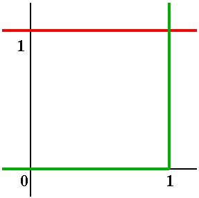
This f(2)/g(2) is about 101,500/1.00014, which certainly looks good for the top -- it is much larger than the bottom. Maple really didn't want to draw this function on the interval [0,1.1]: it objected with the remark "Y axis values too large". So to the right is my diagram of what the graph might look like. x5000 is in green. When x is between -1 and +1, the high power drives the values down down down to 0 (at least as far as the scale in this picture is concerned). But still the value at +1 is +1, so the green graph must go through (1,1). And the darn thing must be continuous. For x>1, the values get really large, very very very fast. So the green graph seems to shoot straight up. What about e.00007x, in red? On the scale shown, this graph seems to be almost a horizontal line at height 1. The thickness of the drawn line conceals any tilt the graph might have. So this is all quite strange, especially if we evaluate the limits.
Log vs polynomials
I did not do this is class, but, time and energy permitting, I should
have.
What is the
limx-->infinity[ln(x)]/[x1/300]?
Before using L'H we must check that some appropriate set of
hypotheses are satisfied. Here certainly ln(x) gets larger when x gets
large "enough" and so does x1/300. That is, the limit of
the top as x-->infinity is infinity, and the bottom has the same
limiting behavior. It isn't hard, by the way, to see that both the top
and the bottom get large. Try a big number (?), like
10100. Then ln(10100)=100ln(10) is approximately
230, and (10100)1/300=101/3 is about
2.15. Well they do get big, but they get big "slowly" and this limit
is essentially asking which of the two, the top or the bottom, gets
bigger slower.
In any case, this is an indeteriminate form of the type,
"infinity/infinity" and we can try to use L'H.
limx-->infinity[ln(x)]/[x1/300]=(using L'H)=limx-->infinity[1/x]/[(1/300)x(1/300)-1].
Let's get rid of the compound fraction in the last expression. We then
need to evaluate limx->300x-1+1-1/300. I think I
did the exponents correctly, and the result is the limit as x-->infinity
of a constant (300) multiplying a negative (-1/300) power of x. The
result is certainly 0.
Therefore we conclude that the limit is 0 and x1/300 gets
bigger faster than ln(x)! But what about the numbers? We just didn't
take numbers that are big enough to see what's happening.
Try (10100)100. A little bit of juggling with
exponents will show that
ln((10100)100)=10,000ln(10) which is about
23,000. And ((10100)100)1/300 is
(10100)1/3 which is about 1033. And
it is true that 1033 is much much bigger that
23,000.
Binary entropy function
Here is one
reference defining the binary entropy function. Google has over one and half million
references to this. The letter p is usually used for the input to H
because the p stands for probability.
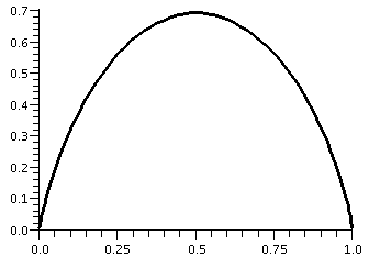 H(p)=-p·ln(p)-(1-p)·ln(1-p) is called the binary entropy
function. It is used when investigating the amount of information
which can be sent through certain communications channels. Usually the
log's involved are logs base 2, but that really doesn't matter here.
Even on a fairly simple level, there are already difficulties: what is the domain of H? Since part of H's formula involves ln(p), certainly p>0. But part of the formula also involves ln(1-p), so 1-p>0 or p<1. So the actual domain of H is just the open interval from 0 to 1, not including its endpoints. A Maple graph of this function is shown to the right. (I think I had this upside down in class, which just shows how badly my brain is functioning).
The point in my discussing this function at this stage of the course is to look at the edges of this graph. The edges seem to suggest that certain limits of H(p) exist and even suggest the values of these limits. For example, it certainly looks like if p gets close to 0 (more officially, p-->0+) then H(p)-->0. Diary entry in progress!
Demons, human beings, and angels
I mentioned this in class but did not go into detail. Here is more
detail, beginning with a metaphor.
The world is made up of a hierarchy (spelling?) of demons and humans and angels. All the demons are less than the humans and all the humans are less than the angels. The "internal" arrangements of {demon|human|angel} society are quite complex, but between the societies things are rather simple.Now onto functions and growth of functions, if you can stop giggling. Let's think about polynomials: x^2 and .002x^3 and -sqrt(5)x^9+98x^10. Polynomials are nice and I think maybe I can almost understand them. They are all a sum of monomials multiplied by constants. As x-->+infinity, what matters is the highest degree term with a positive coefficient, and what matters if two polynomials have a highest degree term of the same degree is what the coefficient is.
Now polynomials are human. What are angels? An angel is a sum of constants multiplying exponentials with constants. So angels are 2e^{3x} and 5e^{.0003x}+99e^{-99x}. These functions also have rates of growth as x-->+infinity, and we can compare two of them in a similar fashion, only here the comparison is first look for a positive coefficient multiplying an exponential with a positive growth number. So .99e^{.03x} is eventually bigger than 9999999999e^{.0003x}.
How are polynomials and exponentials related? Let me stick to things with positive coefficients. A very tiny exponential, say .00001e^{.00000000001x}, compared to a huge polynomial, say 10,000,000,000x^{100,000,000,000}, is bigger, as x-->infinity. Eventually, all angels outrank humans.
Now, continuing in our development of function growth via analogy and idiotic metaphor, let's consider polynomials of log functions: these are functions like 33(ln(x))^{30} and sums of them. Well, these are the demons. EVERY demon is eventually less than EVERY human.
Let me "compare" P(x)=33(ln(x))^{300} with, say, Q(x)=x^{.0001}. Poor Q(x) is a very weakly growing human, as x-->+infinity. And, wow, P(x) is rather a strong demon. Indeed, P(10) is about 1.5 times 10 to the 110th power, and Q(10) is about 1.00023. But let me investigate their "ultimate strength". The simplest way is to consider the limit of P(x)/Q(x) as x-->+infinity. Certainly this is a limit of the form infinity/infinity. so I should L'Hop the whole mess. If I do, the result seems to be:
Top=33(300)(ln(x))^{299}(1/x).
Bottom=.0001x^{-.9999}
I hope I did this correctly. Now let's do some algebra to this quotient. I will put all of the x powers downstairs, and push the constants out to the front. So the result is (I hope):
(ugly constant)
33(300)/.0001 multiplying  (ln(x))^{299} divided by x^{.0001}.
Essentially all I have done is lowered the degree of the demon by 1, and I still want the limit as x-->infinity. I hope you can convince yourself that eventually (after another 299 L'Hops?) that the limit will be 0. This "miserable" human (?) eventually defeats a very powerful demon. It may take a while but this really really happens. For example, I bet (I just experimented in another window of my computer!) that if x is greater than 10^8, P(x) is LESS THAN Q(x). If you object that 10^8 is large, my response will be that there is just as much "room" between 10^8 and infinity and there is between, say, 17 and infinity. And scale of action doesn't matter to demons and humans and angels, only what EVENTUALLY happens.
Sigh. I hope this does help you. It may be more than you want to know but it really is more or less the mathematical truth. The metaphor is just there to help. People who study theoretical computer science and algorithms really worry about the growth of functions. They have the families of functions we have just discussed (called Exp and Poly and Log) but also many others. Sigh. You can look at their zoo if you like, to check that I'm not kidding: the complexity zoo.
A string of definitions with some examples
A situation ...
Rolle's Theorem
| Wednesday, October 25 | (Lecture 15) |
|---|
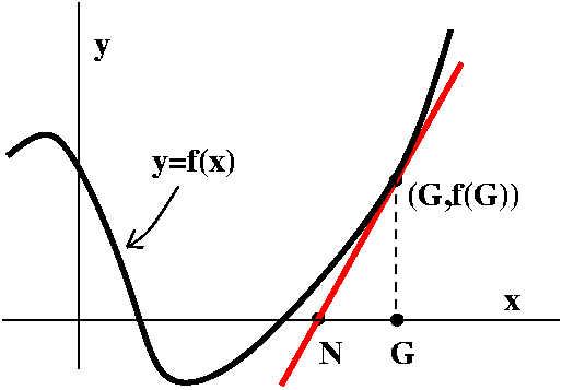 Newton's Method
Newton's method is a way to (try to) improve a guess at a root
of f(x)=0 when f is a differentiable function. The guess, G, is
(hopefully!) improved with the following process (as you read this,
please glance at the picture to the right). First, go up from G
until you "hit" the graph of y=f(x). The point will be (G,f(G)). Then
"slide down" the tangent line of the graph at the pointwhose slope
is f´(G). The point that this line hits the x-axis is the new
guess, N. The picture is rather simple and shows the new guess closer
to a root of the function. This picture is rather simple, and is the
way we would like the method to work. I will discuss more
horrible possibilities later, but right now I would like to get a
formula for N in terms of G. Well, the slope is f´(G), but this
slope is also equal to OPPOSITE over ADJACENT. Here OPPOSITE is f(G)
and ADJACENT is G-N. Therefore
f´(G)=f(G)/(G-N) which is the same as G-N=f(G)/f´(G), so that
| Newton's method N=G-{f(G)/f´(G)} |
|---|
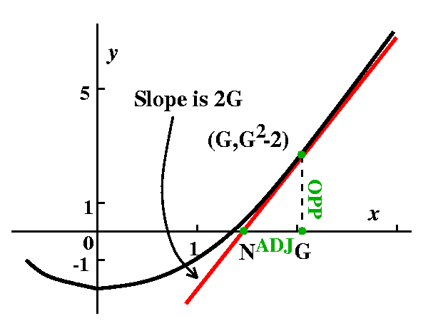
For square roots
Here f(x)=x2-A and f´(x)=2x, so that
G-{f(G)/f´(G)} becomes
G-{[G2-A]/2G} which is
{2G2-[G2-A]}/2G which is [G2+A]/2G
which is (1/2)[G+{A/G}].
That is, "Improve the guess to a new guess, N, by taking the average
of the old guess, G, and A/G: N=(1/2)(G+[A/G])."
Some numerical results
Here is an example, computed by Maple:
I wanted to compute the square root of 2. As is well-known (but not by
me!) this is 1.4142135623730950488 to 20-digit accuracy. My first
guess, A, was 3. Here is a table of next guesses using the Babylonian
method, and the difference between the guess and the true value of
sqrt(2):
| Next guess | 1.8333333333333333333 | 0.41911977096023828453164460912 |
| Next guess | 1.4621212121212121212 | 0.04790764974811707241043248791 |
| Next guess | 1.4149984298948029517 | 0.00078486752170790299608172641 |
| Next guess | 1.4142137800471975839 | 0.00000021767410253511833468993 |
| Next guess | 1.4142135623731118008 | 0.00000000000001675206944769266 |
| Next guess | 1.4142135623730950488 | 0.000000000:27 consecutive 0's! |
Approximating 71/5
Suppose we wanted to compute the fifth root of 7. Sigh. Well, just
suppose. I would like a "simple" function whose root is
71/5. I should be able to evaluate the function and its
derivative "easily", and this certainly suggests polynomials. I think
of f(x)=x5-7 which has exactly one root at 71/5.
Then f´(x)=5x4. The Newton's method "scheme" of
N=G-{f(G)/f´(G)} becomes
N=G-[(G5-7)/5G4]. My faithful silicon companion
(?) "simplifies" this to
(4G5+7)/(5G4).
Some numerical results
71/5 is 1.475773161594552069276917 (to 25 digits of
accuracy). Suppose I use Newton's method with an initial guess of
1. Here are some numerical results:
| Next guess | 2.200000000000000000000000 | 0.724226838405447930723083 |
| Next guess | 1.819763677344443685540605 | 0.343990515749891616263688 |
| Next guess | 1.583474829896161245487585 | 0.107701668301609176210668 |
| Next guess | 1.489460974145427937401052 | 0.013687812550875868124135 |
| Next guess | 1.476022436131861027900625 | 0.000249274537308958623708 |
| Next guess | 1.475773245776608279542563 | 0.000000084182056210265646] |
| Next guess | 1.475773161594561673216009 | 0.000000000000009603939092 |
More phenomena
Newton's method can give some surprising
answers. It definitely should be used, since under good
circumstances it converges very rapidly, but you should be warned that
it can also misbehave.
An example
Here is one example of the use of Newton's
method with quite a simple function, selected to show some problems. I
hope the analysis will not be too hard to understand. If you try a
random polynomial you will probably get very messy results, much more
difficult to understand and analyze than this example. But the example
does show behavior that does happen in general.
The function is
f(x)=x/(1+x2). Let's look at the derivative:
f'(x)=[1·(1+x2)-2x(x)]/[(1+x2)2].
Here it is worthwhile to simplify, since I would like to work with
f'(x). The result is
f'(x)=(1-x2)/[(1+x2)2]. The Newton's
method iteration for going from an old guess, G, to a new guess, N, is
to take G to G-f(G)/f'(G). In this particular case, N=G-f(G)/f'(G) is
G-[x/(1+x2)]/[(1-x2)/[(1+x2)2]].
The second term is a compound fraction. The expression can be
simplified quite a lot with some algebraic work. In fact, for going
from an old guess, G, to a new guess, N, the formula is:
N=(2G3)/(G2-1).
Also notice that y=x/(1+x2/) has a root at exactly one value of x, x=0. What I would like to do now is color the points of the curve green if starting from that point the sequence of Newton's method iterations converges to the only root, 0. I would like to color the points red if the iterations do not converge to 0. I would also like to discuss any weird behavior that occurs.
 Here is a picture (qualitatively correct) of x/(1+x2). |
| Probably geometry may be more of a help to us than the algebra alone. In fact, they should be used together, to reinforce each other. The curve drawn is symmetric with respect to the origin. It has pieces only in the first and third quadrants. So the colors I draw should reflect that symmetry. The analysis I present here uses only two colors and is therefore a bit more simple than what I said in class. I just distinguish between points whose "iterates" approach the only root of 0 and those which get large (both +/-infinity). So here we go: |
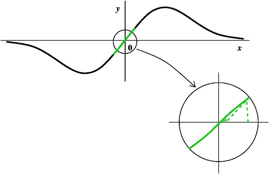 A green point, then some more green points
Certainly, starting with G=0 gets N=0, so that the root itself is green. Are there other green points? Well, drawing a few pictures near O should convince you that if you try starting near 0, the Newton's method iteration rapidly approaches 0. The picture here tries to show that with a few iterations. The interval around 0 is an example of what is called a basin of attraction (really!). |
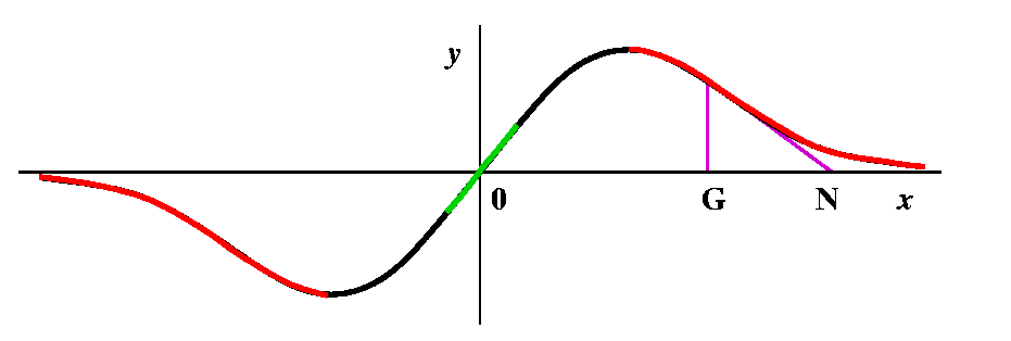 Some red, then some more red points
Suppose we try x=10 as G, our initial guess. Then the formula gives N=(2G3)/(G2-1). How does N compare with G? G seems fairly "large", and the top has twice G cubed, while the bottom only has G squared. I bet that the new guess, N, is to the right of G. In fact, the top of the bump (the maximum, we will officially call it on Monday) is located at (1,1/2) (just see where f'(x)=0 -- remember that f'(x) is (1-x2)/[(1+x2)2], so it is 0 only when the top, 1-x2, is 0, and that is at x=+/-1. So 10 is far to the right. And if G=10, N is even larger, more to the right. For me, looking at the picture is much easier than trying to understand the algebra. And if you look to the right of the top bump, you can see that the tangent lines will all slant "down" (have negative slope) and that therefore for guesses which are bigger than x=1, the new guesses are being driven away from 0, the root. So all of the points on the curve which are bigger than 1 must be red. Of course, a symmetric conclusion is reach for points less than -1, where the iteration drives guesses to the left. |
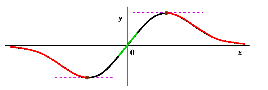 Weird things or not so weird at all
The algebraic formula N=(2G3)/(G2-1) isn't so good when G=+/-1. We are not supposed to divide by 0. What happens in the picture? The tangent lines at those points are horizontal, and they never intersect the x-axis. So maybe I should color those two points some special color just to show that the red/green distinction doesn't apply to them. I guess I will color them brown, a silly color for a silly point. |
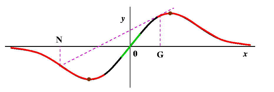 More red in towards 0
Suppose now we look at the curve a tiny bit to the left of where x=1. Then the tangent line has very small positive slope, and will hit the x-axis on the far left. Above that point, the curve is red, and redness spreads contagiously backwards so the point we started with is red. So some part of the left-hand side of the top bump is red, and similarly, by (anti)symmetry, something on the right-hand side of the bottom bump must be red. |
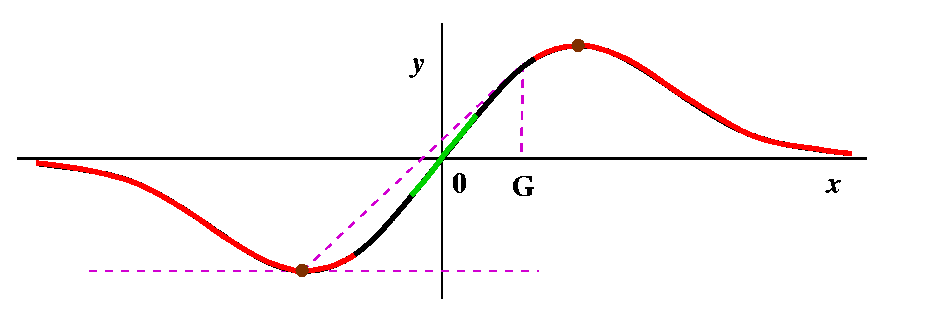 Brown: how can there be more brown?
Keep traveling left on the top bump, in the red stuff. The next new guess will begin traveling right on a part of the curve where x<0. Eventually, though, the line will intersect the x-axis at x=-1. Do you believe me? well, let us solve N=(2G3)/(G2-1) when N=-1. Then 2G3=1-G2 (by cross-multiplying) and so we need to find numbers for which 2G3+G2-1=0. There is exactly one such number (verify this on your own graphing calculator, please) and its approximate value is .657298, so I think since this number is shoved into -1 it should be brown also. And so should its negative, since that gets pushed into +1. |
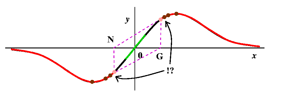 And more red
Push to the left from the previous point. Then the Newton's method iteration takes us into the red region directly to the left of the point on the curve where x=-1. And then, if you can imagine it, further to the left we come to a point which gets pushed into the second brown point on the left. So that point should be brown also, and then there should be a part of the curve which is red and then ... This is very complicated. There are actually on each side of the curve infinitely many intervals of red, and each red interval has brown points on its edge, so there are also infinitely many brown points. The red intervals are getting shorter and shorter, though, until: Something new happens If you look at the picture closely, you will see that there is a positive number G so that when we compute N and then compute N again, the two tangent lines are parallel! For this point Newton's method does not go to +/-infinity and does not go to 0: it oscillates repeatedly. We can even compute this number. By symmetry, at this point, N should be -G, so the equation N=(2G3)/(G2-1) becomes -G=(2G3)/(G2-1) and if we cross-multiply we will eventually get 3G3=G. One root is G=0 which gives us nothing new. The other roots are G=+/-sqrt(3). So I have shown these two points in pink: pink for periodic. In general, Newton's method does have points that sort of wander around, and don't converge to anything, and don't "escape" to +/-infinity. Newton's method can be very complicated. I have also indicated the behavior of infinitely alternating red strips and brown points with !? because I (and all other people!) can't draw this very well. This behavior is an example of a fractal set. |
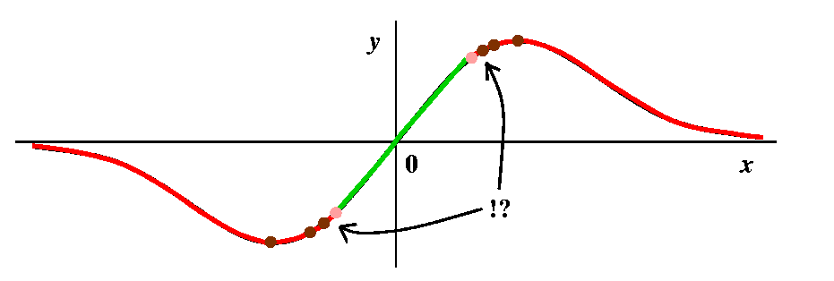
|
| This picture tries to display a completely colored graph. The green points are attracted to the root, 0, by Newton's method. The red points go out to +/- infinity (alternate strips of red go to alternate infinities [here by infinity I just mean eventual travel steadily out to the left or the right]), and each red strip is bordered by brown points which eventually under iteration don't go anywhere (!): they get sent to the wastebasket, outside of the domain of Newton's method. The region labelled !? is too hard to draw, with infinitely many alternations of color. Finally, the two pink points represent points which are alternated with each other periodically by Newton's method. This is already complicated. A "random" function would likely have even more complicated behavior. |
L'H
L'Hopital's (also L'Hôpital's or L'Hospital's) Rule is a method
of evaluating certain very special limits. It is worth showing to you
because it is another neat application of "local linearization", and
some really important limits become easy to evaluate. However, it must
be used with some care. One
quote I found on the Internet declared, "Giving l'Hopital's Rule
to a calculus student is like handing a chainsaw to a three year old."
A motivating example
Let's look at limx-->0[e4x-1]/sin(3x). Of course
I began my consideration of the limit, which is made up of familiar
functions, by just plugging in x=0 in the hope that the functions,
which are individually continuous, will be continuous near and at
0. Since this is an invented example, we get 0/0: no hope.
We can do the following. Remember that f(0+h)=f(0)+f'(0)h+Errf(h)·h where the error term, Errf(h), goes to 0 as h-->0. Also g(0+h)=g(0)+g'(0)h+Errg(h)·h where that error term, Errg(h), goes to 0 also as h-->0.
Now look at the quotient:
 f(x)     f(0)+f'(0)h+Errf(h)·h
------ = -----------------------------
 g(x)     g(0)+g'(0)h+Errg(h)·h
If both f(0) and g(0) are Well, make a into 0 and make b into x. Then f(x)=f(0)+f'(0)x+Err·x where Err-->0 as x-->0. Suppose we try this with f(x)=e4x-1, the "top" function inside the limit above. Since f'(x)=4e4x, we can compute f(0)=e0-1=1-1=0 and f'(0)=4. Then f(0)+f'(0)x+Err·x becomes 0+4x+Err·x. What about the bottom? Here f(x)=sin(3x) so f'(x)=cos(3x)3, and f(0)=sin(3·0)=0 and f'(0)=cos(3·0)3=3. The bottom changes into 0+3x+Err·x. Everything is working out so neatly, of course, because this is an arranged example, but the example was "arranged" so that it illustrates a method which is useful often.
Then limx-->0[e4x-1]/sin(3x) becomes limx-->0[0+4x+Err·x]/[0+3x+Err·x] which (factoring out an x everywhere) is limx-->0[4+Err]/[3+Err]. The error terms are different, but qualitatively they have this common property: as x-->0, both error terms-->0. Now we see "easily" that the limit is 4/3.
The preceding discussion is not a proof, but merely presents heuristic
evidence that the result below is true.
L'Hopital's Rule (version 1)
Suppose that f and g have continuous derivatives, and that
f(a)=g(a)=0 (the eligibility criterion). If
limx-->af'(x)/g'(x) exists, then
limx-->af(x)/g(x) exists and is the same value.
To analyze this kind of limit, we usually look at limx-->infinity. It turns out that L'H works for many different "indeterminate forms": 0/0 is one, and infinity/infinity is another. There are more (please see your text, and see there for more formally stated versions of L'H). I will do more next time.
| Monday, October 23 | (Lecture 14) |
|---|
Today we will investigate two consequences of linearization. Linearization, geometrically, is the idea that if you "zoom in" enough on the correct kind of curve, the result is that the graph of the function will more and more nearly resemble a non-vertical line. Algebraically this corresponds to the definition of the derivative. But (see the September 27 lecture, please) we can "unroll" the definition to a remarkable equation.
Now I considered again a remarkable equation.
| [REMARKABLE] f(a+h)=f(a)+f´(a)h+Err·h |
A silly example
In this example, f(x)=x2. Let us look at f(a+h). In this
case we can compute f(a+h) exactly. It is
a2+2ah+h2. We can "match up" the terms here with
parts of the REMARKABLE equation above. So
f(a)=a2, and since f'(x)=2x, the term f'(a)h is exactly
2ah. The "Err·h" term is h2, and certainly when h is
small, this gets smaller faster than b. A numerical example is
something like (5.01)2 which we compute exactly as 25.1001,
and here a=5 and h=.01. This splits up as
25+.1+.0001=52+2(5)(.1)+(.01)2, and the result
of omitting the last term is a very small error.
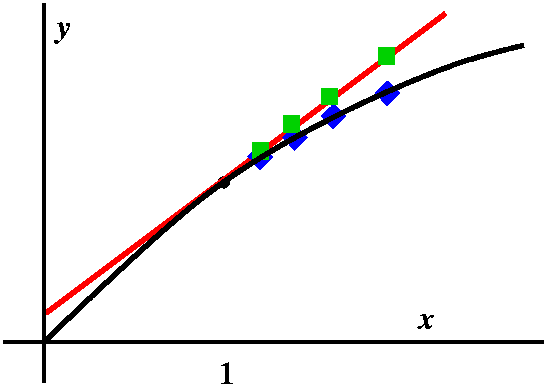
The official name
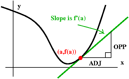
The use of f(a)+f'(a)h in place of f(a+h) is called the linear
approximation to f at a. There are several reasons it is called
the linear approximation. First, algebraic formulas (here thinking of
h as the variable) which only involve constant and first degree terms
are called linear. Second, consider the tangent line to y=f(x) at
x=a. The slope of that line is f'(a). It goes through (a,f(a)). If we
increase a by an amount h, the line's height is increased by f'(a)h
(because OPP/ADJ is f'(a) and ADJ is h in the right triangle
shown). So the linear approximation gives a formula which instead of
using the correct value of f(a+h) substitutes the value obtained by
"extrapolating" using the value on the tangent line.
Another example, perhaps less silly
What is the square root of a number close to 1? Since square root is a
continuous function, such a value of square root should be
approximately the square root of 1, which is 1. But how should we
"correct" the answer if we want sqrt(1+x) for x small? Here we have
f(x)=sqrt(x) and a=1. So we need f'(1) which is easy, since
f'(x) is (1/2)x-1/2 and f'(1)=1/2. Therefore the linear
approximation to f(a+h), that is, to sqrt(1+h), is just 1+(1/2)h. Now
I tried to do some arithmetic. The following table is somewhat more
extensive than I computed in class with student help. Here my help was
Maple and the computations were done to 30 digits accuracy. (!)
| Values of h | "True" values of sqrt(1+h) | Linear approximation values: 1+(1/2)h | 3rd column - 2nd column |
|---|---|---|---|
| 1.5 | 1.2247448713915890491 | 1.25 | -0.0252551286084109509 |
| 1.05 | 1.0246950765959598383 | 1.025 | -0.0003049234040401617 |
| 1.005 | 1.0024968827881710675 | 1.025 | -0.0000031172118289324 |
| 1.0005 | 1.0002499687578100594 | 1.00025 | -0.0000000312421899406 |
| 1.00005 | 1.0000249996875078123 | 1.000025 | -0.0000000003124921877 |
| 1.000005 | 1.0000024999968750078 | 1.0000025 | -0.0000000000031249922 |
| 1.0000005 | 1.0000002499999687500 | 1.0000005 | -0.0000000000000312499 |
One more example
Finally, I asked what happened to the
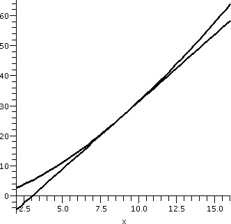
three-halves powers of numbers near 9. Here f(x)=x3/2, so
f'(x)=(3/2)x1/2. If a=9 and h is a small number, we can
hope that (9+h)3/2 is close to f(9)+f'(9)h. Since f(9)=27
(hey, I chose 9 because the 3/2's power of 9 is "simple") and
f'(9)=(3/2)(3)=4.5, we now know that (9+h)3/2 is
approximately 27+(4.5)h. This may or may not be interesting to you,
but if you need to really think about many values of x3/2
near 9, this approximation provides some insight. I also can tell you
that this approximation is an overestimate of the true value,
since x3/2 curves "up" and the tangent line at (9,27) is
under the curve. A picture that Maple drew of this situation
is to the right. We will soon learn how to tell if the tangent line is
underneath or over the curve without looking at the graph. As one
numerical example, the linear approximation to (8.96)3/2
is 26.820 because this is 27+(8.96-9)(9/2), and the "true" value seems
to be about 26.82020, just a bit more (as the picture shows).
An implicit function example
How your calculator computes square roots: some possibilities
I asked how a calculator computes square roots. Most of the answers I
got were, "By pushing the button," but I repeated my question. Here
are my suggested answers.
Babylonian square roots
Here is a complete description of the process:
How to compute the square root of A to a specified
amount of accuracy
The method initially looks quite weird: replace G by (1/2)(G+[A/G]. Well, is it? First, if your "guess" is too large (so G2>A) then G>sqrt(A) and (G/A)>(1/sqrt(A)) so that (A/G)<sqrt(A). We are averaging numbers that are on either side of sqrt(A). So maybe we will get closer. The amazing result is that we get very much closer, very fast, and I will substantiate this with some numbers next time.
| Wednesday, October 18 | (Lecture 13) |
|---|
Mostly descriptive but now analytical.
puerile trivial, childish, immature.
A cube with edge length changing
A rain drop evaporating
Running on the square root curve
Leaving Hoboken
Now: a rectangle that does everything!
The exam comes back
| Sunday, October 15 | (Review session) |
|---|
Maintained by greenfie@math.rutgers.edu and last modified 10/16/2006.