I did not verify that there is such a number (e, that is). But the
following "argument" provides one way to approximate it.
If we
took the 100th power (raised things to the 100) then the
1/100 and 100 in the exponent of e cancel (repeated
exponentiations multiply) so that
e is about
(1+{1/100})100.
This is, by the way, 2.704813829. Well, you can see it in the
accompanying table. This method of "computing" or approximating e is
actually very very slow. The first
several million digits of e are online, if you need them.
Then I worked on building new functions. If F(x)=f(x)+g(x), and the
derivatives of f and g exist, what can one predict about the existence
and value of the derivative of F?
Since F(x)=f(x)+g(x) we know that F(x+h)=f(x+h)+g(x+h), and the difference quotient for F can be written this way:
(F(x+h)-F(x))/h=[(f(x+h)+g(x+h))-(f(x)+g(x))]/h=[f(x+h)-f(x)+g(x+h)-g(x)]/h=[f(x+h)-f(x)]/h+[g(x+h)-g(x)]/h.
And now let h-->0, and we see that the derivative of the sum is the sum of the derivatives.
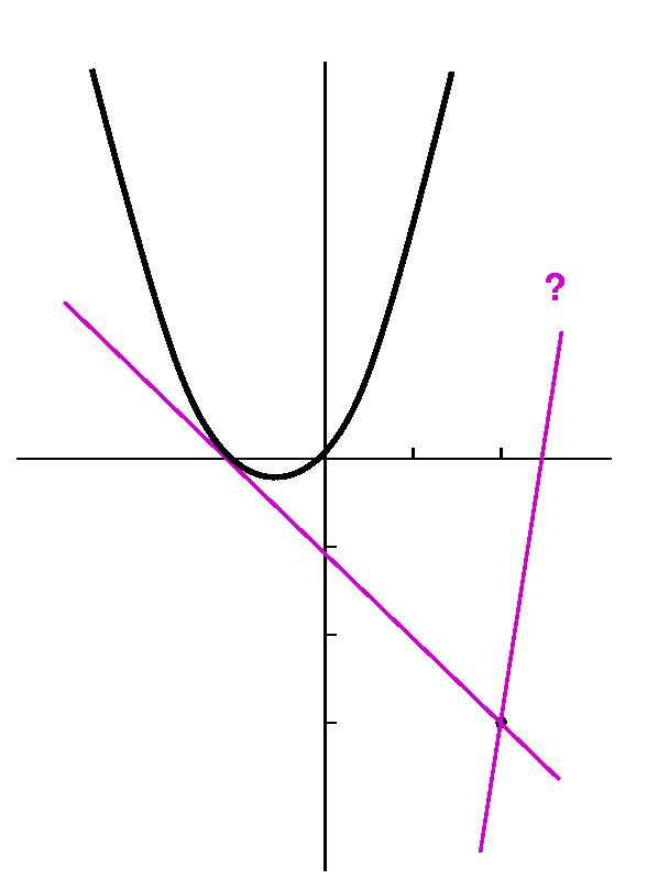
Now I did a hard problem from the textbook (I think #50 of
section 3.1), to show that we have gotten already to some level of
achievement. The problem asks us to find the equations of the lines
tangent to the parabola y=x2+x which also go through the
point (2,-3). Note that although the problem statement does not
request it, I would almost always begin the solution by making a
sketch.
If P=(x,y) is the point of tangency on the parabola, we can solve the
problem by realizing that the slope of the tangent line at P,
mTAN, can be written in two different ways. First,
since the tangent line goes through P and (2,-3), its slope is
(y-(-3))/(x-2), which is (x2+x+3)/(x-2). But
mTAN is also f´(x) if f(x)=x2+x. So
mTAN=2x+1. Therefore
2x+1=(x2+x+3)/(x-2), and
(2x+1)(x-2)=x2+x+3. Then
2x2-3x-2=x2+x+3 so that moving everything to one
side, we get x2-4x-5=0. Since this is a problem in a
textbook, the quadratic factors into (x-5)(x+1)=0. If x=5, then
y=52+5=30 and the derivative is 2(5)+1=11. So the tangent
line is y-30=11(x-5). We can make a cheap check: does this line go
through (2,-3)? Well, -3-30=-33 and 11(2-5)=-33, so the answer is
"Yes." The point of tangency is (5,30) which explains why we can't see
it in the picture. You can find the equation of the other line
yourself.
Now we began to discuss what is called the product rule. The
statement of the product rule begins "The derivative of the product is
..." There is an expectation of simplicity and symmetry here, which
should be eliminated as soon as possible. Consider x2 which
is also, of course, x·x. The derivative of x is 1, and
1·1=1, but the derivative of x2 is 2x, so the
product of the derivatives is not the formula we want.
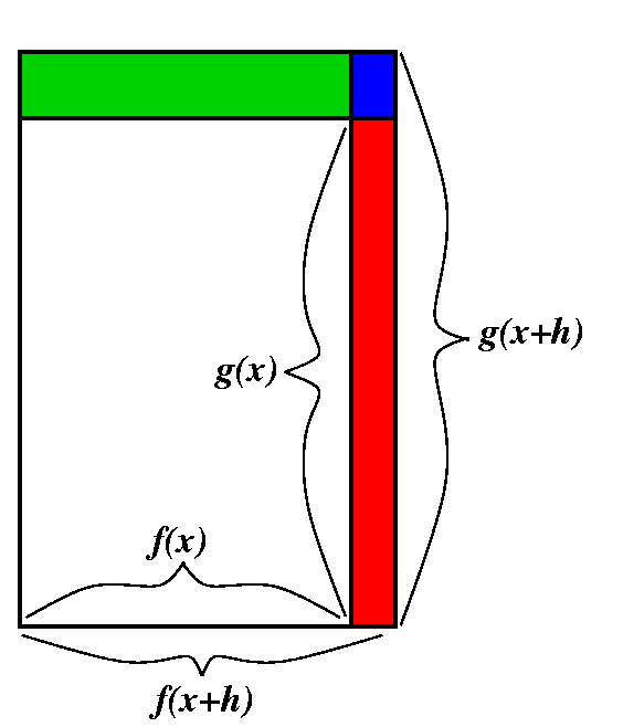
If F(x)=f(x)·g(x), then F(x+h)=f(x+h)·g(x+h), so that
(F(x+h)-F(x))/h=(f(x+h)·g(x+h)-f(x)·g(x))/h. Now the
game is to somehow write this fraction in terms of the difference
quotient of f and the difference quotient of g. Here the picture may
help. It tries to show a sort of decomposition of
f(x+h)·g(x+h)-f(x)·g(x). The suggestion is that
f(x+h)·g(x+h)-f(x)·g(x)=(f(x+h)-f(x))·g(x)+f(x)·(g(x+h)-g(x))+(f(x+h)-f(x))·(g(x+h)-g(x)). If we now divide
by h and let h-->0, then:
[(f(x+h)-f(x))·g(x)]/h-->f´(x)·g(x) and
[f(x)·(g(x+h)-g(x))]/h-->f(x)·g´(x).
The blue rectangle in the corner is a curiosity. It is algebraically
(f(x+h)-f(x))·(g(x+h)-g(x)) (then divided by h)
In the [REMARKABLE] equation I mentioned last time:
F(x+h)=F(x)+F´(x)h+Err·h the blue rectangle belongs to the Error term. So what happens is this:
[(f(x+h)-f(x))·(g(x+h)-g(x))]/h=[(f(x+h)-f(x))/h]·(g(x+h)-g(x)). The first term -->f´(x) but the second term: g(x+h)-->g(x as
h-->0 since g is continuous (because differentiable functions are continuous).
Therefore the blue rectangle divided by h -->f´(x)·0 which is 0: it contributes nothing to the limit. This is a bit elaborate, but I'd like to be honest
when I can be (!?). So now we know that the derivative of f(x)·g(x) is
f´(x)·g(x)+f(x)·g(x). This is called the product rule or, sometimes, the Leibniz rule, memorializing one of the inventors of calculus.
Examples: If f(x)=x and g(x)=x, the product rule gives us
1·x+x·1=2x, the correct answer. We can also
differentiate something like ex·x178. And
we can differentiate 37·x23 with f(x)=37 (a constant
function) and g(x)=x23. The product rule predicts that the
derivative is
0·x37+37·23x22. Frequently people
use this special case of the product rule without thinking about it:
the derivative of a constant times a function is a constant times the
derivative of the function.
| Wednesday,
September 27 | (Lecture
#7) |
|---|
Don't treat infinity like a number!
I had remarked that "statements" like
limx-->infinityf(x)=L
should be understood more as abbreviations of geometric descriptions
than anything else. Therefore treating infinity as a number, adding or
multiplying or whatever, may give "results" which are deceptive or
even incorrect. I wanted to emphasize this and decided to show some
examples using the following functions.
f(x)=x g(x)=sqrt(x2+1) h(x)=sqrt(x2+x)
I hope that you would agree with me that each of these functions have
the property that, as x-->infinity, the function will also
-->infinity. I mean specifically the following quantitative
relationship:
If you choose any positive number M, no matter how large, then I can
choose a positive number N so that if x>N, then the function will
be >M.
For example, suppose I wish to exhibit this for the function
g(x)=sqrt(x2+1). You tell me you want this function to be
larger than 10,000. Well, if I want to force
sqrt(x2+1)>10,000 then (square) this is the same as
x2+1>100,000,000 and this is the same as
x2>100,000,000-1. Well, let me "forget" the -1. If I
only knew that
x2>100,000,000 then x2>100,000,000-1
also.
So how can I make x2>100,000,000? Just take
x>10,000. So I can make g(x) big by making x big.
One example
I'm going to look at g(x)-f(x). This is sqrt(x2+1)-x. I
want to investigate
limx-->infinity sqrt(x2+1)-x.
"Clearly" (always use that word when you can't explain where the idea
comes from) multiply this by a fraction which has the same thing on
the top and the bottom (so the fraction is a fancy way of writing
"1".) Here the following fraction was suggested:
sqrt(x2+1)+x
-------------
sqrt(x2+1)+x
I was told that the top and bottom were each the conjugate of
the formula for g(x)-f(x). Then
                            (sqrt(x2+1)-x)(sqrt(x2+1)+x)
g(x)-f(x) = sqrt(x2+1)-x = ------------------------------- =
                                  sqrt(x2+1)+x)

   (x2+1)-x2               1
----------------- = ---------------
   sqrt(x2+1)+x)     sqrt(x2+1)+x
(Here we are using (A-B)(A+B)=A2-B2
with A=sqrt(x2+1) and B=x. The final fraction
shows us that the result -->0 since the bottom grows to "infinity".
Therefore limx-->infinityg(x)-f(x)=0.
Another example
Now let me look at h(x)-f(x). This is sqrt(x2+x)-x. I'd
like to consider
limx-->infinity sqrt(x2+x)-x.
Now the appropriate conjugate is (sqrt(x2+x)+x).
                            (sqrt(x2+x)-x)(sqrt(x2+x)+x)
h(x)-f(x) = sqrt(x2+1)-x = ------------------------------- =
                                  sqrt(x2+x)+x)

   (x2+x)-x2               x
--------------- = ---------------
  sqrt(x2+x)+x)    sqrt(x2+x)+x
Here things are bit more complicated.
Now look:
sqrt(x2+x)=sqrt(x2[1+{1/x}])=sqrt(x2)sqrt(1+{1/x}).
We've seen sqrt(x2) before, and what is it? If x is
positive, then sqrt(x2)=x. (If x were negative,
sqrt(x2 is -x.) Here we go:
      x               x                              x                    1
-------------- = ------------------------- = ------------------- = -------------------
 sqrt(x2+x)+x     sqrt(x2)sqrt(1+{1/x})+x     x[sqrt(1+{1/x})+1]    [sqrt(1+{1/x})+1]
Take a look at the last bit of "mess". The only appearance of x is in
1/x, and certainly as x-->infinity, this should-->0. All of the other
pieces of the expression don't change. If you carefully examine them,
you will see that the result is 1/2.
Therefore limx-->infinityh(x)-f(x)=1/2.
Numerical evidence?
I haven't talked enough about numerical evidence for limits in class,
mostly because I am scared of using a calculator or computer in front
of people. But I certainly use such things on my own. So here is some
numerical information.
| | x=10 | x=102 | x=103 | x=104 | x=105 |
|---|
| sqrt(x2+1)-x |
0.0498756211 |
0.0049998750 |
0.0004999998 |
0.0000499999 |
0.0000049999 |
|---|
| sqrt(x2+x)-x |
0.4880884817 |
0.4987562112 |
0.4998750624 |
0.4999875006 |
0.4999987500 |
|---|
 I needed 25 digit accuracy to get the last few entries in the first
row to 10 digit accuracy. Computations with small numbers which are
almost equal can be imprecise. But the numbers should help you
accept the previous results which were obtained with algebraic
manipulation.
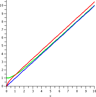
If you prefer graphical evidence then maybe the picture to the
right can help. It shows graphs of f(x)=x and g(x)=sqrt(x2+1) h(x)=sqrt(x2+x) on the interval
[0,10]. Although 10 is not very large, I think the asymptotic
relationships between the functions are already apparent.
Short cuts are good but ...
So I know limx-->infinityx=infinity and
limx-->infinitysqrt(x2+1)=infinity,
but limx-->infinitysqrt(x2+1)-x=0.
And I also know limx-->infinityx=infinity and
limx-->infinitysqrt(x2+x)=infinity,
but limx-->infinitysqrt(x2+x)-x=1/2.
Please notice that 1/2 and 0 are not
equal.
Therefore for this kind of limit, simple algebraic manipulations
are not guaranteed to give valid results. We all like
computational shortcuts, but limits involving infinity can be
difficult to manipulate. Such limits should be treated more as
descriptions of geometric situations rather that anything else.
Vocabulary?
On a well-known web page (concerning the Fungi
of Australia, the word conjugate is defined to mean
"copulation, especially isogamic copulation". I think I am too scared
to look up "isogamic" since it might mean something illegal.
How to evaluate limits
As was remarked in the previous lecture, if the limiting function were
defined with familiar formulas, I'd first try to "plug in" if there is
any chance this strategy can be applied. If this simplest method can't
be used, I'd try to "massage" the function (algebraically) and get to
some algebraically equivalent restatement where plugging in can be
used.
The derivative
Here is the most important single use of limit in Math 151.
Suppose f(x) is a function. Then we write f is
differentiable at x=a if
limh-->0[f(a+h)-f(a)]/h exists. If the limit exists, it is
called the derivative of f at a and
the notation f´(a) is used for
the value of the limit.
Comments There are other notations for the derivative (almost
every chunk of applied science and engineering has its favorite
notation!). We'll see some of them. Please notice that the quotient
involved in the definition of the derivative is exactly of the
form which prevents direct "plugging in". If we insert h=0 in
[f(a+h)-f(a)]/h we get [f(a+0)-f(a)]/0 and that's 0/0, a meaningless
arithmetic expression.
One nice example
Suppose f(x)=1/x2. We already looked at this function in
the lecture on September 13 (whose diary entry is not done, which I
regret). Let's look at [f(a+h)-f(a)]/h:
                        1         1
                     -------  - -----
  1/(a+h)2-1/a2       (a+h)2      a2
----------------  = ------------------
        h                 h
My goal is to understand what happens to this as h-->0. If I
"plug in" h=0 now I get no information. I will use part of my brain to
manipulate this mess algebraically, and hope that I will eventually
get to an equivalent algebraic form whose behavior as h-->0 will
be apparent (by plugging in: that would be the easiest thing). Now
what we have here is a compound fraction, and I will convert it to a
simple fraction (with one "division"). Experience tells me that's
easier to understand.
    1         1          a2-(a+h)2
 -------  - -----      -------------
 (a+h)2      a2          (a+h)2a2          a2-(a+h)2
------------------- = --------------- = --------------
       h                   h              h(a+h)2a2
The major "transition" here is done by multiplying
the top and bottom each by 1/h, and the resulting fraction
has 1 in the bottom and is therefore a "simple" fraction. Now we
expand part of the top, cancel a2 additively and h
multiplicatively:
  a2-(a+h)2       a2-[a2+2ah+h2]      -2ah-h2        h(-2a-h)      -2a-h
------------- = ---------------- =  ----------- = ------------ = --------
  h(a+h)2a2        h(a+h)2a2          h(a+h)2a2     h(a+h)2a2    (a+h)2a2
Now finally I can "plug in" h=0. More properly for this course,
I can see what happens as h-->0. The limit does exist, and
its value is -2a/{a2a2]. Usually people write
this as -2/a3.
We have verified that f(x)=1/x2 is differentiable, and
that f´(x), the derivative of f, is -2/x3.
Comments There are many opportunities to make algebraic
errors in what's done above. One amazing thing is that we will develop
very easy ways to compute derivatives for almost all familiar
functions combined in interesting ways (including algebraic
combinations and composition and "inversing"). Most of next week will
be devoted to stating and understanding these results. Although you
should (and will, darn it!) practice these rules (algorithms!),
learning them is not the peak of the course. There are very nice
programs which can compute such derivatives. A major purpose of the
course is to understand why derivatives are interesting to
people. We need to know how to use them. And maybe machines are not
yet up to that level of cognition.
Not a nice example
Consider f(x)=|x|. I would like to see if this f is differentiable at
a=0. Therefore I must consider:
f(0+h)-f(0)    |0+h|-|0|    |h|
----------- = ---------- = -----
    h              h         h
I need to understand what happens to |h|/h as h-->0. Any computations
with absolute value will go better if they are split into two parts,
one from each side.
| h<0 so we are considering h-->0- |
h>0 so we are considering h-->0+ |
| Here h is negative, and |h|=-h. Therefore |h|/h is -h/h and this
is -1: there's no appearance of h in this result. I think that the
limit as h-->0- of |h|/h must be -1.
|
Here h is positive, and |h|=h. Therefore |h|/h is h/h and this
is +1: there's no appearance of h in this result. I think that the
limit as h-->0+ of |h|/h must be +1.
|
But the limits from the two sides (+/-) don't agree. Therefore the
limit limh-->0[f(0+h)-f(0)]/h does not
exist.
We conclude that this function is not differentiable
at x=0.
Interpretations
Here are a collection of simple interpretations of what we are
discussing. Other interpretations will be shown in you in virtually
every technical course you take from now on.
| Math 151 | Geometry in the plane | Simple physical
motion |
|---|
| We're given some function f, and want to understand how it
"changes". |
The object studied is the graph of f, which is the collection of
points in the plane with coordinates (x,y) which satisfy y=f(x). |
Here we study rectilinear motion, where the position
of a point on the coordinate line is given by f(x) (usually the
variable is called t, not x, because this would help people remember
that f(x) is the position at time "x").
|
| The change in f over an interval from a to a+h is just f(a+h)-f(a).
| f(a+h)-f(a) denotes the difference in the heights of the
function at the x-values a and a+h.
|  f(a+h)-f(a) is the difference in position at the two times
indicated. This is also called displacement. In general, this
is not the distance that the point travels between those two
times, because the moving point could wiggle back and forth.
|
| [f(a+h)-f(a)]/h is called the average rate of change of f
over the interval.
| 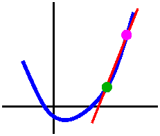 [f(a+h)-f(a)]/h is the slope of the secant line through the
points (a,f(a)) and (a+h,f(a+h)).
| [f(a+h)-f(a)]/h is called the average velocity of the
point over the time interval.
|
|
If, as h-->0, the average rate of change of f approaches a
limit, this limit is called the derivative of f at a and
written f´(a).
| 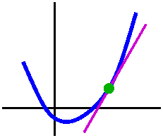 If, as h-->0, the slope of the secant line approaches a
limit, this limit is called the slope of the tangent line to y=f(x)
at x=a.
| If, as h-->0, the average velocity of the
point over the time interval approaches a limit, this limit is called
the instantaneous velocity of the point at the time x=a. The
limit in this case is frequently written ds/dt (difference in s, a
Latin abbreviation for distance, divided by a difference in t, meaning
time.
|
I will usually abbreviate the word "instantaneous" while discussing
velocity, because I will almost never again refer to average
velocity.
O.k.: a tangent line
Well, I made a mistake in class. I will not repeat the mistake
here. Here I will use a different function. I will try hard not to
make another mistake.
Suppose f(x) is the function defined by the formula
sqrt(17+x3). Then it turns out that this function is
differentiable (if you are "naive" this is not at all obvious and
would be quite difficult to verify directly from the definition!) and
f´(x)=[3x2]/[2sqrt(17+x3)]. Please: we will
very soon see how this formula gets computed! Suppose I ask for an
equation of the line tangent to the graph of this f(x) when x=2? We need some
information.
A point on the line Well, (2,f(2)) is a point on the line, and
f(2)=sqrt(17+23)=sqrt(17+8)=sqrt(25)=5.
Slope of the line Well, f´(2) is supposed to be the slope
of the tangent line, and this is
f´(2)=[3·22]/[2sqrt(17+23)]=3·4/[2·5]=6/5.
Therefore an
equation of the line tangent to the graph of this f(x) when x=2
is (y-5)=[6/5](x-2). I am lazy and I will not "simplify".
Some numerical "work"
Very very very few of you will need to write the equations of tangent
lines after getting through a first calculus course. But you will
almost certainly need to consider many, many derivatives and make
judgements based on these derivatives. What the heck is going on?
Well, let us think about the example above. Since f´(2)=6/5, I
know that
limh-->0[f(2+h)-f(2)]/h=6/5.
If I omit the "limh-->0" phrasing, then the equality is no
longer ture. But the limit definition implies that what is true is a
statement with an error term, and this error term is small when h is
small. That is:
[f(2+h)-f(2)]/h=6/5+{ERROR [small when
h is small]}. I can multiply by h and then add f(2)
and get the following equation:
f(2+h)=f(2)+(6/5)h+{ERROR [small when
h is small]}h
This equation is really why people study derivatives. The important
qualitative aspect is that the Error is multiplied by h, and when h is
small the Error is small. Products of "smalls" are even smaller, and
the effect on the output of changing the input to f by h for small h
is almost entirely determined by the multiplier, (6/5)h. Here are some
numbers.
Input value
x |
 | Output
value
f(x)=sqrt(17+x3) |
|---|
|
| x=2 |
f(x) is exactly 5. |
| x=2+h |
f(2+h)=f(2)+(6/5)h+{ERROR [small when h is small]}h |
| x=2.1 so h=.1 |
f(x) is about 5.124548 and
f(2)+(6/5)(.1) equals 5.12 |
| x=2.01 so h=.01 |
f(x) is about 5.012045 and
f(2)+(6/5)(.01) equals 5.012 |
| x=1.9 so h=-.1 |
f(x) is about 4.884567 and
f(2)+(6/5)(-.1) equals 4.88 |
| x=1.99 so h=-.01 |
f(x) is about 4.988045 and
f(2)+(6/5)(.01) equals 4.988 |
|
Reinterpreting the definition
The function f is differentiable at a if for any very small
{perturbation|kick|change} to the input, h, the output will be
approximately f(a) (the old output) plus a constant multiplying the
perturbation. That constant is the derivative of f at a.
Monday, September 25
Diary entry in progress!
Thursday ...
Students will need to hand in a writeup of a workshop problem and
several textbook problems. They will also have a computational test
about limits. An example of the test
is available, as are answers .
The strategies available now for computing limits are:
- "Plug in": if the function is given by a formula involving
standard functions and you know the darn thing is continuous.
- Transform what's given using standard algebraic manipulations into
a form where you can "plug in".
- There will be some other strategies, later.
Intermediate Value Theorem, restated
Suppose that the function f is
defined and continuous on the interval [a,b]. Then the equation f(x)=y
has at least one solution for every y which is between f(a) and f(b).
QotD, version 2 (fill in the blanks)
The QotD last time was not suitable. Here, maybe is something I should
have asked, an alternative QotD for the last lecture, with a
fill-in-the-blanks format.
Suppose
f(x)=x3+cos(7x2+5)+sin(3x4-8)+2.
Then
f(-2) is # 1
because (-2)3=-8 and the remainder of the formula
describing the function f(x) is at most # 2 at x=-2.
And
f(+2) is # 3 because 23=8
and the most negative the remainder of the formula describing
the function f(x) can be at x=2 is # 4 .
Since f(x) is # 5 in the interval [-2,2]
and the signs of f(x) at the endpoints differ, f(x) must have
# 6 root in [-2,2].
So the QotD would have been to fill in the blanks. Here we go:
- negative
- 4: the
"outputs" of sine and cosine are between +1 and -1, and therefore
cos(7x2+5)+sin(3x4-8)+2 must be somewhere in the
interval [-4,4]. The "stuff" inside the sine and cosine terms is
mostly irrelevant here.
- positive
- -4: the
reasoning is the same as for #2.
- continuous
- at least one
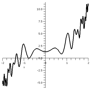
To the right is a graph of y=f(x) on the interval [-2,2].
Indeed, there is "at least one" root inside the interval. Actually,
there seem to be several roots.
Horizontal and vertical asymptotes: geometric and algebraic
vocabulary
The limit idea was fairly successful, and people over years decided to
use it to cover more and more situations. Sometimes the extensions
were not as simple as the original setting. One extension that is
useful describes certain geometric behavior of graphs called vertical
and horizontal asymptotes.
Near x=3
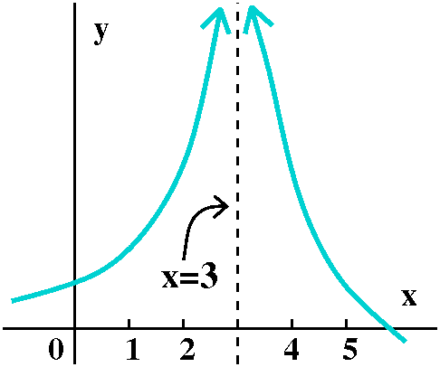 To the right is the graph of a function, f(x), whose
domain includes all x except for 3. The "arrows" at the top of the
curve are supposed to indicate that as x gets closer and closer to 3
(on either the right or the left side) then f(x) gets large. But
there's more, really. It doesn't just "get" large in some uncontrolled
way. The function is
supposed to
-
Get as large as "you" want So if any number is named
(10? 100? 100,000? 1010?), the function gets larger than
that number close enough to 3.
- Stay large Not only does it get large, but eventually it
stays large. For example, the graph is supposed to indicate that there
is some (perhaps small) positive number, epsilon, so that if
0<|x-3|<epsilon, then f(x)>1010. This is, for me,
difficult to imagine.
If both the "get large" and "stay large" statements are valid, then
x=3 is a vertical asymptote of f(x). And, further, this geometric and
numerical situation is abbreviated algebraically by
limx-->3f(x)=infinity.
I add immediately that I am not declaring that "infinity" is a
number. I am merely telling you that this particular limit statement
is supposed to be an abbreviation of the geometric situation shown.
Examples
1/(x-3)? 1/|x-2|?? 1/(x-3)2???
1/(x-3)EVEN POS INT???
A rational function
x2/[(x+2)3(x+4)6]
Horizontal asymptotic behavior
Be a bit careful ...
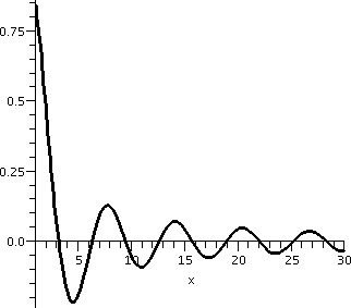 sin(x)/x
Not damned oscillation, just damped oscillation
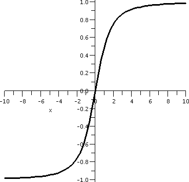 x/sqrt(x2+3)
Wednesday, September 20
Diary entry in progress!
Review of the definition of limit
Discussion, criticism, comments about the definition of limit
Framework of ideas supporting the definition of limit
Algebra
Order (1)
Wiggling
Squeezing the wiggling
Order (2)
Plugging in
An important official word: continuity
The Garden State Parkway, from Cape May to Montvale
and my friend Francine ...
 The
Garden State Parkway runs most of the length of New Jersey. Mile
0 is at Cape May, while the other end, mile 172, seems to be close to
Montvale. Suppose that my friend Francine leaves Cape May at 7 AM one
morning, and drives north on the Garden State Parkway. Further,
suppose she arrives at mile 172, the northern end, at, say, 10
AM. Must Francine at some time be at mile 135 (fairly near Busch
campus)? The parkway seal here was "borrowed" from a State of New
Jersey webpage.
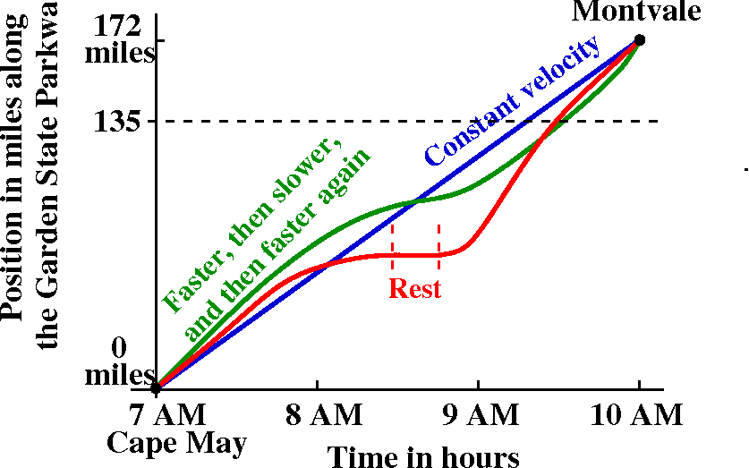 We discussed various curves which could represent the position of
Francine on the parkway in terms of miles from the start of the
parkway at time t, in terms of hours elapsed from 7 AM. I tried to
show that our everyday intuition lead to the graph being
increasing (as you travel from left to right, the points on
the graph go up). The graph can have level spots, where Francine pulls
over for a rest stop. Legally Francine isn't supposed to drive
backwards, though.
If we believe that motion is continuous (so Francine does not
have a Star Trek transporter or other device) then the graph of
Francine's position goes from (7 AM, 0 miles) to (10 AM, 172 miles)
and therefore the graph must have on it at least one point with
coordinate description (*,135). All of this, by the way, rests on some
complicated assumptions, some of them philosophical (why should
motion be continuous?). Today, though, I believe that motion
is continuous, and therefore at sometime Francine must be at Mile
135. By the way, I will retain this information for later, when we
analyze the rate of change of position (velocity) so that we can see
whether Francine deserves a speeding ticket.
The Intermediate Value Theorem
Suppose that the function f is
defined and continuous on the interval [a,b]. Then the equation f(x)=y
has at least one solution for every y which is between f(a) and f(b).
In mathematics, the word theorem is applied to results that are
deduced from basic principles, and usually the term is used for more
important conclusions in the subject. In this case, the Intermediate
Value Theorem follows from basic principles governing the real
numbers. A particular basic principle which is used in the proof of
the theorem is the "least upper bound" property of the real
numbers. This essentially declares that there are "no holes" in the
real numbers. A precise statement is fairly delicate, and this
property essentially shows that the reals and the rationals are
distinct. Several upper-level math courses spend quite a bit of time
exploring the statement. You can read about it in
Wikipedia but I do add that detailed knowledge of such
foundational material is not needed for success in Math 151 (or, for
that matter, for successful careers in almost all of science and
engineering!).
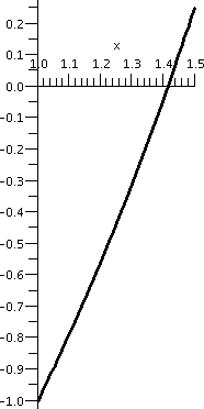
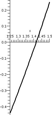
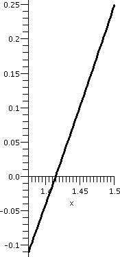
The square root of 2
If we were desperate to compute
sqrt(2) (that is, really, desperate to approximate sqrt(2)),
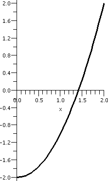
for example, we could look at f(x)=x2-2 on the interval
[0,2]. This f(x) is certainly continuous. (We already observed that we
could "plug in" values to evaluate limits for polynomials. I know that
f(0)=-2<0 and f(2)=+2>0. Therefore according to the Intermediate
Value Theorem there will be at least one x inside the interval [0,2]
so that f(x)=0: x2-2=0. This is a positive number whose
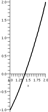
square is 2, which we call sqrt(2). Now we have "trapped" sqrt(2)
inside the interval [0,2]. If we compute f(1)=12-2=-1, we
know that a root must be inside [1,2] since the signs of f(x) at the
two endpoints differ. We can continue this "game", each time halving
the interval, and chosing a half-subinterval so that the signs of f(x)
differ on the endpoints. The graph of f(x) on the first few
subintervals is shown below.
| Interval: [0,2] |
Interval: [1,2] |
Interval: [1,1.5] |
Interval: [1.25,1.5] |
Interval: [1.375,1.5] |
|---|
 |
 |
 |
 |
 |
The bisection method for root-finding
I discussed this too rapidly and then asked the QotD about it. I
regret the hurry. In particular, I mentioned the word "algorithm". Let
me give some further information about this word in the form of quotes
from
The Art of Computer Programming by D. E. Knuth:
The modern meaning for algorithm is quite similar to that
of recipe, process, method, technique, procedure, routine,
except that the word "algorithm" connotes something just a little
different. Besides merely being a finite set of rules which gives a
sequence of operations for solving a specific type of problem, an
algorithm has five important features:
- Finiteness An algorithm must always terminate
after a finite number of steps.
- Definiteness Each step of an algorithm must be
precisely defined; the actions to be carried out must be rigorously
and unambiguously specified for each case.
- Input An algorithm has zero or more inputs, i.e.,
quantities which are given to it initially before the algorithm
begins. These inputs are taken from specified sets of objects.
- Output An algorithm has one or more outputs, i.e.,
quantities which have a specified relation to the inputs.
- Effectiveness An algorithm is also generally
expected to be effective. This means that all of the operations
to be performed in the algorithm must be sufficiently basic that they
can in principle be done exactly and in a finite length of time \e
Knuth continues on the same page to contrast his definition of
algorithm with what could be found in a cookbook:
Let us try to compare the concept of an algorithm with that of a
cookbook recipe: A recipe presumably has the qualities of
finiteness (although it is said that a watched pot never boils), input
(eggs, flour, etc.) and output (TV dinner, etc.) but notoriously lacks
definiteness. There are frequently cases in which the definiteness is
missing, e.g., "Add a dash of salt." A "dash" is defined as "less
than 1/8 teaspoon"; salt is perhaps well enough defined; but
where should the salt be added (on top, side, etc.)?
... a computer
programmer can learn much by studying a good recipe book
| Discussion of the bisection algorithm |
Specification of the bisection algorithm |
|---|
|
The bisection algorithm is one of the simplest and neatest
algorithms. It approximates roots very nicely. The entry conditions
are a continuous function defined on an interval which includes the
interval's endpoints. Also the sign of the function at the endpoints
differs: the function's value is positive at one endpoint and negative
at the other. Then, according to the Intermediate Value Theorem, there
must be at least one root (f(x)=0) inside the interval. Another entry
condition is a positive number, here called epsilon, which serves as
the error tolerance for the root.
|
Entry conditions
A continuous function f(x) defined on an interval [a,b], with
f(a)·f(b)<0;
a positive tolerance epsilon for the error.
|
| Here we check if the interval we're looking at already
fulfills the error tolerance condition. In later steps, we will be
altering the interval, and shrinking it.
| Exit condition
If b-a<epsilon, report the interval [a,b] as the answer.
|
|
Compute the value of f(x) at the middle of the interval.
| Computation
Let c=(1/2)(a+b). Compute f(c).
|
| Here's the heart (?) of the algorithm. If f(a) and f(c) have
different signs, then the root desired is in [a,c], the left half of
the interval. We then change the interval (shrinking it) and see if
the length of the interval is small enough. If the signs of f(a) and
f(c) are not different, the root we're looking for (whose presence is
guaranteed by the Intermediate Value Theorem!) is in the right
half of the interval. So we redefine [a,b] as the right half interval
and check if the exit condition is satisfied.
| Decision
If f(a)·f(c)<0, then change b to c, and return to check the Exit
condition.
Otherwise, change a to c, and return to check the Exit
condition.
|
Monday, September 18
Office hours
My formal office hours will be from 10:30 to noon on Wednesday and
Thursday. These are times when I will try to definitely be in
my office (or, sigh, in the building, at least!). You can certainly
talk to me before or after class, or communicate by e-mail, if you'd
like to see me at other times. I will most likely be on campus most
days.
Workshop work ...
Workshops are important, as I've said previously. And they will be
graded (by the recitation instructor and by me) equally for both
mathematical content and technical exposition. Please try to do both,
and please ask for advice about writeups from either of us.
Textbook homework assignments
The textbook homework assignments to be handed in on a Thursday should
be available each week on Monday. I hope this will help you schedule
your work.
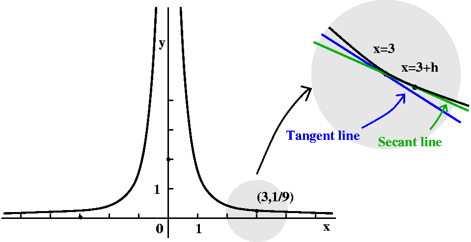 Slope of a tangent line
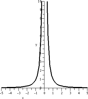
Let's look at the curve y=1/x2 near x=3. The point (3,1/9)
is on the curve, since 1/32=1/9. We can try to find the
equation of a line tangent to the curve at (3,1/9). Since we know a
point this line goes through, we will be able to find an equation for
the line if we know a slope. I'll call the slope of the tangent line
mtan. The traditional calculus way to find this slope is to
approximate it with msec, the slope of a secant line. This
will be a line which goes through the point (3,1/9) and
(3+h,1/(3+h)2) when h is small. We can get this slope by
writing it as the difference in the second coordinates divided by the
diffeence in the first coordinates:
   1      1
 ----- - ---
 (3+h)2 - 9
--------------
   (3+h)-3
I'd like to see what happens when h gets very very small. In the
geometric picture the secant line is held down at (3,1/9) and as h
gets small, the secant line will sort of revolve into the tangent
line, and msec will get close to
mtan. Algebraically, if I inspect the quotient I've just
written and try to quickly see the behavior as h gets small by
replacing h by 0, the result will be 0/0, and we can't assign any
value to this quotient. But let's try some simple algebra on the
quotient, first replacing the compound fraction by an equal simple
fraction:
   1      1            9-(3+h)2
 ----- - ---         -----------
 (3+h)2 - 9            9(3+h)2            9-(3+h)2
--------------  =  --------------  =  ---------------
   (3+h)-3              h                 h9(3+h)2
Now let's "expand" the top and cancel the 9's.
 9-(3+h)2        9-(9+6h+h2)        -6h-h2
-----------  =  -------------  =  -----------
 h9(3+h)2         h9(3+h)2          h9(3+h)2
But we can cancel factors of h from the bottom and from the top (we must cancel an h from both terms on the top).
  -6h-h2        -6-h
---------  =  ---------
 h9(3+h)2      9(3+h)2
Now the "asymptotic" nature of the fraction shouldn't be too difficult
to see: when h gets close to 0, the top of the fraction gets close to
-6 and the bottom gets close to 9·9=81. So I think that
mtan should be -6/81, which is -2/27.
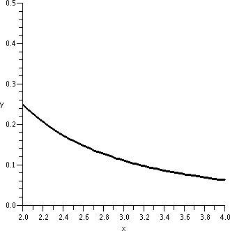
Is mtan=-2/27 "reasonable"? Well, if we look at the graph
we can see that the y values on the curve are getting smaller as the x
values increase (near x=3). So the tangent line should tilt down,
which makes the minus sign of the answer more agreeable. The magnitude
of the slope, 2/27, is small, and, in fact, if you really look
at the curve, the tilt is quite small. Some graphs are shown below. Of
course 0 is not in the domain of 1/x2.
| y=1/x2; x between -5 and 5 |
y=1/x2; x between 2 and 4 |
y=1/x2; x between 2.9 and 3.1 |
 |
 |
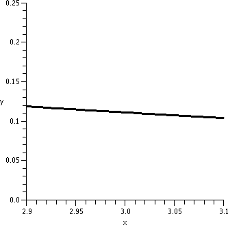 |
The graphs need to be looked at a bit carefully. The vertical interval
in the first graph is [0,20]. In the second graph it is [0,.5], and in
the third graph it is [0,.25]. This graph is locally
linearizable near x=3 in the following sense: if we "zoom in" on
it near the point (3,1/9) a sufficient number of times, the graph will
look as near to a straight line as we would like. The line that
results will got through (3,1/9), and will have slope -2/27.
 Possibly the slope of another tangent line
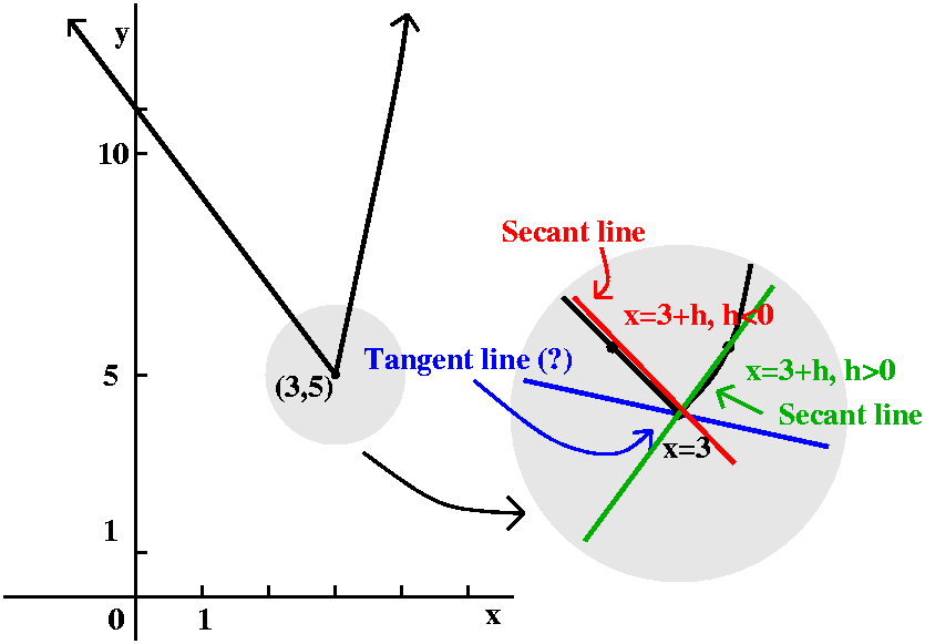
Suppose now that we define f(x) in a piecewise fashion:
      11 -2x if x<3
f(x)=
      x2-4 if x≥3
Now the analysis of the slopes of the approximating secant lines is
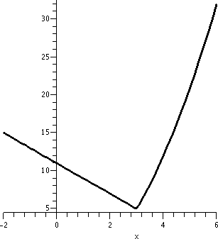
more complicated. A graph of the function (with lots of other "stuff")
is shown to the right. The point (3,5) is on the graph, and the point
(3,5) also satisfies y=11-2x and y=x2-4. There is no jump
or break in the graph at (3,5). Please note, though, that the vertical
and horizontal scales differ. Let's analyze msec if h>0:
 f(3+h)-f(3)      (3+h)2-4-5        9+6h+h2-9
------------  =  ------------  =  -----------  =  6+h
      h                h               h
Therefore as h gets small (with h positive) msec seems to
get close to 6. So 6 seems to be our candidate for mtan.
msec if h<0:
 f(3+h)-f(3)       11-2(3+h)-5        11-6-2h-5
-------------  =  --------------  =  ------------  =  -2
      h                 h                 h
Therefore msec seems to be -2.
There does not seem to be one value of mtan here. So I
guess there may not be a unique satisfactory tangent line. Some
pictures may help.
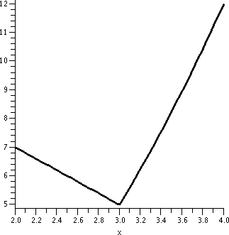
| y=1/x2; x between -2 and 6 |
y=1/x2; x between 2 and 4 |
y=1/x2; x between 2.9 and 3.1 |
 |
 |
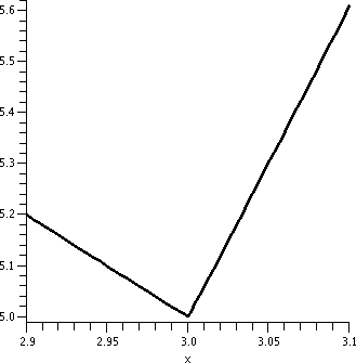 |
Again look closely at these pictures, which all have differing
horizontal and vertical scales. In this case, there's no amount of
"zooming in" which will make the graph look like a straight line
segment. This graph is not locally linerizable. The behavior is
qualitatively very different from the previous example.
Limits
The relationship between the approximating msec and
mtan needs to be investigated more precisely. There's a
name to the process: LIMIT. Limits are
fundamental to precise statements about asymptotic relationships of
all kinds.
 Exactness and reality
"Real" functions are not very exact. A chemical engineer might have
(I'm simplifying hugely) some process which produces the correct kind
of plastic if, say, a certain amount of benzene is used in the
mix. (Hey: benzene, with chemical formula
X3Y7Z11 (nah), was suggested by a
student. So a certain percent of benzene, say 3%, may produce a
plastic which has the desired amount of, say, translucence. But in
reality, even very precise measurements may not create an input with
exactly 3% benzene. Maybe some days we get 3.5, or 4.2. And maybe the
desired output measurement is not necessary -- we can deal with some
error in the output. Real measurements imply that we need to
contemplate error, not as a moral defect (at least in this case), but
as part of our mathematical model which we must deal with.
Output tolerance as controlled by input tolerance
So maybe we need to understand the following idea: we want a
certain output tolerance: that is what we can "live with" in the
material created. Is there an input tolerance describing inputs in an
interval around the ideal input which makes the corresponding outputs
close enough to the desired output? This is too darn abstract. Let me
consider a numerical example, with a very simple function.
x2 near x=3
|
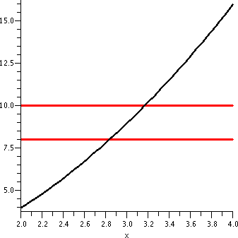
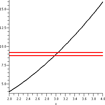
If the input to f(x)=x2 is 3, the output will be 9. Suppose
we are willing to live with a +/- error of 1 in the output. That is,
we can tolerate |f(x)-9|<1. Is there some simple specification of
an interval of inputs near 3 which will guarantee this? In this case,
almost everyone thinks that the simplest kind of input specification
would be an interval of x's centered at 3 (your feelings may differ
here, but this is what is usually done). So I ask if there is some
convenient number ("CN") so that if |x-3|<CN then
|x2-9|<9. Most people don't want an exact, precise, most
perfect (?) value of CN. It may be difficult to get something like
that. They are willing to settle for something convenient. In this
case, the graph to the right shows the needed output tolerance using
horizontal red lines.
|
|
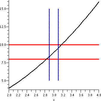
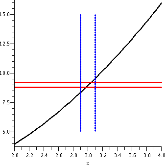
The next graph, shown here to the right, adds part of the vertical
lines corresponding to x=2.9 and x=3.1. The part of f(x)=x2
shown which is between the vertical blue lines is "clearly" forced to
be between the red horizontal lines. This geometry reflects the
following algebraic statement:
If |x-3|<.1 then
|x2-9|<1.
So an input tolerance of .1 around 3 will guarantee that the output
tolerance of 1 around 9 is true.
|
 |
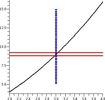
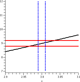
Change the output tolerance to .2
What if we changed the desired output tolerance to .2? That is, we
want to get |x2-9|<.2 by controlling the size of |x-3|.
x2 near x=10
Now let me change the game a bit. Suppose I want to consider the same
function, f(x)=x2, but now investigate what happens near
10. Since f(10)=100, the "ideal" input is 10 to get the "ideal" output
of 100.
|
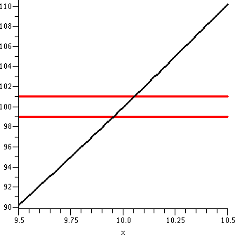
Suppose I want the outputs to be within 1 of the ideal output. That
is, I want |x2-9|<1. The horizontal lines shown indicate this restriction.
Warning!
There is a huge horizontal/vertical distortion in this graph. The
horizontal scale ranges from 9.5 to 10.5, a length of 1. The vertical
scale goes from about 90 to about 110, a length of 20. The "true"
picture is a long and thin vertical rectangle, with a 1-to-20 aspect
ratio.
|
|
|
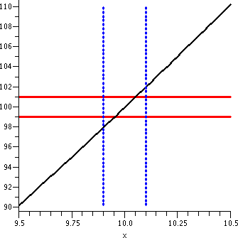
The vertical lines shown are x=9.9 and x=10.1, which would be the
geometric side of the input restriction |x-10|<.1, the input
tolerance we used in "If |x-3|<.1 then |x2-9|<1" The
same input tolerance won't work about different "ideal inputs". If you
really believe in the graph, this isn't too surprising since the graph
is much more tilted around x=10 than it was around x=3.
|
|
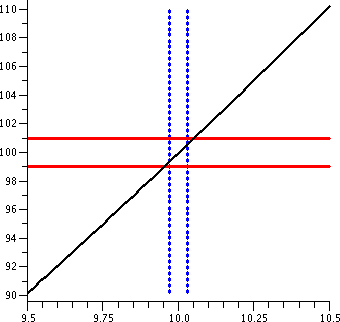
The vertical segments shown are parts of the lines x=9.97 and
x=10.03. I hope this is pictorial evidence that the following
implication is correct:
If |x-10|<.03 then
|x2-100|<1
An input tolerance of .03 satisfies the output tolerance of 1 near the
ideal input/output pair (10,100).
|  |
Complicated? Yes, it is.
These pictures should convince you that the limit business when
addressed "officially" is indeed complicated. In your courses and
careers, there may rarely be times when you'll need to cope with these
implications. But I believe you should have some idea of what's going
on.
Graphs don't really work too well for complicated functions or
irritating input/output pairs. People have therefore developed
extremely intricate strategies relating the inequalities
needed. Serious investigation of this algebra is not the aim of the
course but the equipment is there when/if you need it.
The official definition
The statement limx-->af(x)=L means:
Given any (positive) output tolerance,
there is a (positive) input tolerance so
that
If 0<|x-a|<the input tolerance, then
|f(x)-L|<the output tolerance.
Comments
The traditional algebraic abbreviations for "output tolerance" and
"input tolerance" are the Greek letters epsilon and delta. So the
definition above is frequently called the epsilon-delta definition or
criterion.
I also slipped in a slight change: on the input side, what's needed is
"{ 0<|x-a|<the input tolerance". The 0<|x-a| requirement was
not mentioned before. That's put in primarily because the most
immediate use we will make of limits will be to compute slopes of
tangent lines, what are called "instantaneous rates of change". In
that use you should see already that we sometimes will not be able to
just "plug in" the ideal input (otherwise we'll get a 0/0
situation). So plugging in the ideal input is NOT part of the
definition!
Wednesday, September 13
Diary entry in progress!
The piecewise linear function
The inverse(s)
Example
Some trig functions and their inverses
Some exponential functions and their inverses
Dwarf apple trees
Growth rate
Ultimate height
Chapter 2 and its fictions
Slope of a tangent line
QotD
Monday, September 11
More background
I discussed some of the purposes for some of the things I will do in
this course.
The diary
I mentioned the diary and remarked that it served several
purposes. First, even very enthusiastic students may sometimes miss a
class. The diary can help them find out what was covered. Another
reason for the diary's existence is so that I can fix errors which I
will certainly make, so while the diary will be a representation of
what went on in class it won't be a totally accurate one: improvements
may occur! Also, even if I don't make a mistake in the lecture,
sometimes I may not explain things optimally, so the diary may give
students another chance to understand the presentation. I really don't
think that a diary entirely takes over the teaching/learning aspect of
the lectures. There is still a good amount to be said about the
interaction between the instructor and the student, provided that
students are willing to ask questions and (sigh!) the instructor is
really willing to listen and answer. I will try to do the latter (also
with errors, of course, since I plead the defects of humanity!).
QotD
Most days I will ask students who attend the lecture a question or
two, and receive their answers in writing. Students will get full
credit for any answer. This "Question of the Day" has several
purposes. First and most minor, it is a way of taking
attendance. More important is that it serves as an additional method
of communicating between the lecturer and the audience. If I ask some
question which I think is "simple" and, hey, almost no one answers
the question correctly, well ... something's wrong. I will "grade" the
question very roughly, only retaining for records whether or not an
answer was made. For the student, this gives an opportunity to see if
some content in the lecture has been learned satisfactorily, and, if
not, maybe that also signals that something's wrong. I'll try
to get the graded QotD's back to you in recitation.
Study groups
I asked students in the class to tell me their e-mail addresses and
likely majors, and, with appropriate permission, this information is
now displayed on a web page. Now at the
beginning of this course, there may be little that is new to
students. I caution you, though, that even if you have seen much of
this material before, the course will move swiftly. It is a good idea
to form study groups meeting at appropriate times and durations to go
over homework, etc. I hope that the student list will help people get
in touch with each other.
Calculus [Advertisement]
Calculus originated as a way of describing certain methods used in
understanding and solving problems originating in geometry and
physics. The language of the subject shows this ancestry. Calculus has
been very successful. Calculus also "happens" to be suitable to
describe and study many problems in biology and economics. Any
problems which involve rates of change (how soluble is substance A in
substance B as the concentration of substance C varies?) or
accumulation of changes (what is the present value under
certain interest rate assumptions of a stream of mortgage payments to
be made monthly over the next 20 years?) is a problem which likely can
be described using calculus. Frequently this description will suggest
certain ways of solving the problems using the methods of
calculus. That's why the subject is required in so many majors.
Functions
The word function is used in a technical sense in calculus, and
is one of the most important vocabulary words. It is the logical
setting for how things are transformed to other things. In the case of
Math 151, the "things" are numbers. So functions will change numbers
to numbers. I decided to begin with what I hoped was a known example
described verbally.
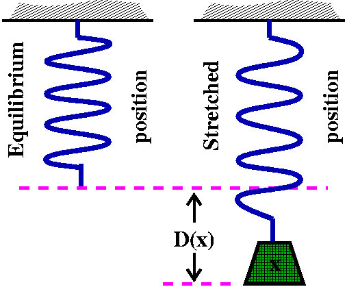
Hooke's law
Think of a spring with a rest or "equilibrium" position. Then Hooke's
Law states that the deviation from the rest position is in direct
proportion to the impressed force. There are many assumptions involved
in Hooke's Law, but to a considerable extent it is a widely valid
shorthand for a great variety of real phenomena. If I further add something like: the spring gets stretched 10 inches by a weight of 300 pounds, then I can formulate an equation relating the impressed force and the deviation from the equilibrium position:
D(x)=(1/30)x
Here D(x) is the deviation in inches from the
equilibrium position (with positive meaning the spring is forced to be
longer) and x is the impressed force in poinds (I'm thinking maybe of
a thick mechanical spring or something like that). x is called the
independent variable and D(x) is called the dependent variable. Notice
that sigh matters. If x is negative, then we could be compressing the
spring, and the end of the spring is higher than the equilibrium
position in our model.
Notice that as in all mathematical models, you need to be alert a bit about how "correct" this is. Uhhh ... if we stretch a rubber band with a force of six trillion tons, I don't necessarily think it will end up having a length of one lightyear.
Functions
 One metaphor I will use (and probably overuse!) in this course is the
idea of a function as a machine with an input and a unique output
associated to each input. The collection of all valid inputs to the
machine, those inputs which don't cause the machine to break, is
called the domain. The collection of all of the outputs for
these valid inputs is called the range.
Functions via formulas
Functions can be described simply with formulas. Actually, most of the
functions we will study in this course will have such
descriptions. Warning: students interested in obviously experimental
disciplines (engineering, physics, chem, etc.) will mostly encounter
functions which are described by data sets, and must work with them
using the techniques of this course which will mostly be presented
using functions defined by formulas. This can be ... irritating.
The domain of a function defined by a formula is usually assumed to be
what's called the natural domain: this is the collection of all
inputs of real numbers which make sense in the formula. But
there will be exceptions (see below!).
- Polynomials
Polynomials are sums of constant multiplies of monomials. So on
example of such a function is
f(x)=53x40-9.7x2+88. Polynomial formulas only
involve multiplication and addition, and therefore the natural domain
of a polynomial is all real numbers.
Exception!
Already, even in such a simple setting, we can have exceptions. Let's
consider the following paragraph, which is really the beginning to a
typical "toy" calculus problem:
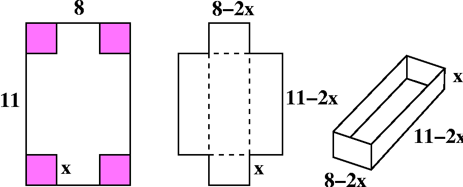
Equal-sized squares are cut from the corners of an 8 inch by 11 inch
rectangular piece of paper. The flaps in the resulting piece of paper
are folder up. Write a formula for the resulting volume which the
paper object encloses, using the edge length of the squares as the
independent variable. What is a useful domain for this formula?
I hope that the accompanying illustrations are helpful. I'll call the
edge length x. Then the "solid" brick will have volume, V(x), which
will be the product of the area of the base multiplied by the
height. The height is x, and the base has sides with lengths 8-2x and
11-2x. So V(x)=x(11-2x)(8-2x). This formula is "just" a polynomial of
degree 3. But please notice that x=-50 or x=200 makes no sense in this
problem. The physically reasonable domain, the x's that can actually
be used, are just those x's in the interval [0,4]. So already here is
an example of a function given by a formula where the applicable
domain for the mathematical model is much smaller than the natural
domain. You may think that this is unreasonable, and I'm being much
too picky. But the restriction is essential.
I was asked by one alert student to describe the range of V(x). I
refused and said I'd need to wait a week or two until we officially
had the correct technical equipment. Until then, I recommended that
many sheets of paper have squares cut from them, many little
containers be created, and then measure the volumes (fill with water
or maybe popcorn?).
- Rational functions
These are quotients of polynomials, for example
f(x)=(x4+6)/(x2-5). Since we are now "allowed" to
divide, we'd better avoid dividing by 0. Here we need to find out
where x2-5=0 which is x=+/-sqrt(5). So the domain is all
other x's: the intervals (-infinity,-sqrt(5)), (-sqrt(5),sqrt(5)), and
(sqrt(5),infinity). Things can get complicated, especially because if
you give a "random" polynomial, finding the roots exactly may not be
possible!
- Algebraic functions
Here we allow roots to occur, so we can get things like
f(x)=sqrt(x2-5). Since even powers can't be negative, we'd
better have inputs to square roots (and other even roots) be
non-negative. So here we need x2-5≥0, which means that
the domain needs to be (-infinity,-sqrt(5)] and [sqrt(5),infinity).
- Exponentials and logs
We'll deal more with these in the future, but exponentials are always
positive, so the domains of logs have restrictions to only positive
numbers. These functions are needed to model many sorts of growth
problems.
- Trig and inverse trig functions
So we need to consider sine and cosine and tangent (domain restricted
to not allow division by 0) in order to model periodic phenomena. The
inverse trig functions have various kinds of domain restrictions.
 Piecewise defined functions
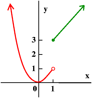
Here is a silly example:
      x2 if x<1
f(x)=
      x+2 if x≥1
Such examples will be useful to consider when we look at
limits. Here f(-2)=(-2)2=4 and f(5)=5+2=7.
Part of the graph of this function is shown to the right. Please note
the "empty circle" on the parabolic arc, because of the restriction
x<1 (x is not allowed to be equal to 1). There's a "filled circle"
on the other piece, a half line.
A more elaborate "real" example
Now here is a somewhat more complicated example:
f(x)=
     .1x if 0≤x≤15,100
     1,510+.15(x-15100) if 15,100<x≤61,300
     8,440+.25(x-61300) if 61300 <x≤123,700
     24,040+.28(x-123700) if 123,700<x≤188,450
     42,170+.33(x-188450) if 188450<x≤336,550
     91,043+.35(x-336,550) if 336,550<x
This is the U.S. individual
tax rate schedule (form 1040) for 2005. The function has many
weird numbers in it. This is an example of a piecewise linear
function because each of the pieces is defined by a polynomial of
degree 1. The slopes of the pieces increase as the x's increase
because this is a progressive income tax. But the other strange
numbers are caused by a desire to avoid jumps and breaks in the graph
of the tax function, so that strange situations don't arise (examples:
yes, you earn $1 more and therefore will pay $100 less in taxes,
etc.).
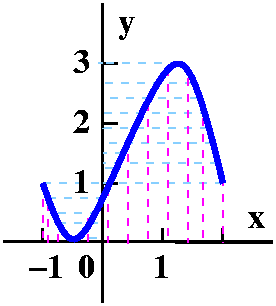
Graph of a function
The graph of a function is the collection of all points in the plane
with coordinates (x,f(x)) if x is in the domain of the function. To
the right is the graph of a function. A collection of points in the
plane is the graph of a function if every vertical line which
touches the graph intersects it exactly once. This is called the
Vertical Line Test, and corresponds to the fact that we want exactly
one output determined by every "legal" input. If we have the graph,
the domain is all x's on the x-axis for which the vertical line
through that x hits the graph. Similarly the range is all y's on the
y-axis for which the horizontal line through that y hits the
graph. Sometimes if you only have the graph and no other information,
precise descriptions of the domain and range can be difficult.
An inverse function
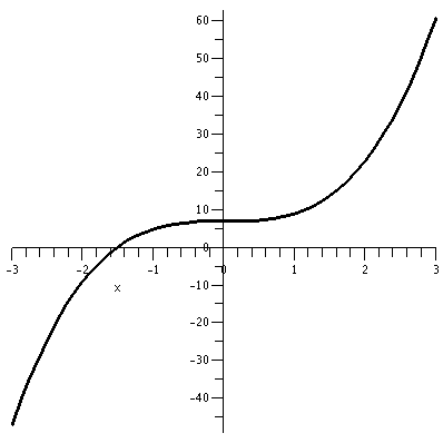
Consider the function defined by f(x)=2x3+7. Part of the
graph of this function is shown to the right. It was produced by my
silicon friend, Maple. (Available on eden, just type
maple). The graph is a bit deceptive. I asked that the
function be shown for x's in the interval from -3 to -3. The program
automatically "autoscales" and squeezes so that the image is in a
square. This can be confusing at times if you don't realize it. In
this case, the vertical range seems to be between -45 and 60.
|
|
The part of the graph I want to emphasize here is the qualitative
aspect: certainly every vertical line hits the graph once (the
Vertical Line Test) but so does every horizontal line. That is, every
output corresponds to a unique input. For this function, this
uniqueness claim can be verified algebraicaly quite easily: if w is an
output, we can write a formula for the unique x it came from.
w=2x3+7 --> w-7=2x3 --> (w-7)/2=x3 -->[(w-7)/2]1/3=x
A function which has unique outputs for each input is called
1-to-1. Such a function has an inverse.
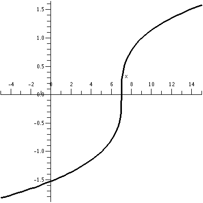
The function g(w)=[(w-7)/2]1/3 is inverse to f. It
undoes f, so that f(g(w))=w and g(f(x))=x. The graph of g is shown to
the right. It is gotten algebraically by interchanging the two
coordinates of each point. Geometrically the graph of the inverse
function is gotten by picking up the original graph of f and "flipping
it over" the main diagonal, y=x.
|
|
 A piecewise linear function to play with
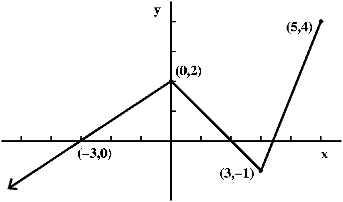
I defined a function by sketching its graph, as shown to the right. I
declared that the function, f(x), was piecewise linear. One part was a
half infinite line (a ray) passing through (-3,0) and ending at
(0,2). Then there was a line segment from (0,2) to (3,-1), followed by
a line segment from (3,-1) to (5,4). The domain of this function was
(-infinity,5] and its range was (-infinity,4]. My real intention was
to use this function to study the problems involved in specifying
inverses, but ...
QotD
Suppose H(x)=f(x2) and K(x)=f(x)2. I asked
students to tell me the domain and range of H and K.
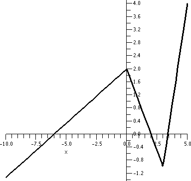
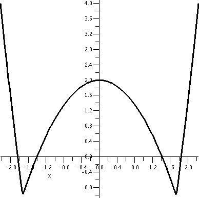
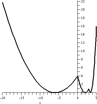
Below, by the way, are graphs of f and H and K, as Maple "sees" them. Notice again that vertical and
horizontal scales differ.
| Graph of part of f | Graph of all of H | Graph of part
of K |
 |
 |
 |
QotD answers
Let's see: H(x)=f(x2). The inputs to f are
(-infinity,5]. But squaring makes things non-negative, so the only
numbers I can push into x so x2 feeds into f are numbers
which won't square to bigger than 5. Therefore I should put in only
numbers between -sqrt(5) and +sqrt(5). So the domain will be
[-sqrt(5),+sqrt(5)]. The range will be the outputs of f when the
inputs of f are in the interval [0,5], and those outputs are [-1,4].
K(x)=f(x)2. Now K has the same domain as f: (-infinity,5]
because the domain of squaring is every possible number -- there are
no restrictions to worry about. The outputs, however, are squared. The
collection of outputs of f(x) are (-infinity,16]. When these are
squared we will get every non-negative number.
Here is more detail. For x>0, the outputs of f(x)2
go from 0 to 16. On the left, though, the outputs of f itself
go down to -infinity, so squaring means the results are all
non-negative numbers. The range of K is [0,infinity).
Wednesday, September 6
We wasted some time giving an "exam" which will be used to
help the math placement process. I believe this is a good thing
although I disliked using class time.
Numbers
- Positive integers
We can start with 0 (the "additive identity": anything plus 0 is
that anything) and 1 (the "mulitplicative identity": anything times 1
is that anything). 1's added to 1's create the positive integers.
- Integers
If subtraction is considered, then we need "additive inverses". The
additive inverses of the positive integers are negative
integers. These together with 0 are all integers.
- Rational numbers
Now multiplicative inverses force the consideration of reciprocals of
integers (except for 0, because that would lead to real algebraic
difficulties). Further multiplication makes the collection of rational
numbers.
- All the others (these are most of them!)
Rational numbers have finite or repeating decimal expansions. In this
course we will use various sequential approximation processes, and we
will need to consider numbers with all sorts of decimal expansions,
not just repeating expansions. These weird and "chaotic" numbers are
not rational: they are irrational. In various ways which can be
made quite precise, there are many more irrational numbers than there
are rational numbers: a typical number is irrational. Any physical
experiment or process when measured gives only an approximation to
some sort of "true" answer, and this sequence of approximations, like
the decimal expansion, is likely to be an approximation of an
irrational number.
Geometry
The real numbers are usually thought of as corresponding to a specific
geometric object, the real line. I usually think of this line
as horizontal with 0 sitting "in the middle". 1 is to the right of
0. And this geometric picture brings up the idea of order. In addition
to the algebraic structure, there is order: a<b. To me this means
(in my picture of the line) that a is to the left of b. Negative
numbers are to the left of 0 and positive numbers, including all the
positive integers, are to the right of 0. Here are some interesting
aspects to note.
The decimal expansion of a real number provides an "address" to locate
the number geometrically. For example, 23.4680472... means we first
move right from 0 by 23 steps, each 1 long. Then look between 23 and
24, and divide that length in tenths. The number we're looking for
resides (?) in the 4th subinterval. Now divide that
subinterval into tenths. The number is in the 6th
subinterval of that collection. Etc. The "Etc." of course conceals an
approximation process which will locate the real number with the
specified decimal expansion.
Some real numbers have two valid decimal expansions. This doesn't
bother me, since, say, a house on a corner of a grid system of streets
could also possibly have two valid addresses (if it is on the corner
of Cedar Avenue and Third Street, the house could have the address 12
Cedar Avenue and also 42 Third Street). So, for example, the real
number with decimal address 23.45999... (with the 9's repeating) also
have the decimal address 23.46, a terminating expansion (there are a
string of 0's which are usually not written.
Distance including a discussion of | |
The distance between two points is a non-negative real number whose
size expresses how far apart the numbers are. This will be important
when we study approximation schemes. We'd like to know that the
approximation gets "close" to the correct answer, and the closeness
will be measure by the distance. Algebraically, if the points
correspond to the real numbers a and b, the distance between them is
|a-b| and this is the same as |b-a|, so that distance has some
symmtery. But I just used absolute value, and here is the
piecewise definition of absolute value:
|x|=x if x≥0 and |x|=-x if x<0
Therefore absolute value is always a non-negative number. The absolute
value of a number is 0 only when the number itself is 0. And absolute
value of a product is the product of the absolute values (this
actually is not totally obvious, and needs a bit of thought, I
believe).
Intervals
Suppose we want to discover what numbers x are closer to 9 than a
distance of 4. Algebraically this requirement translates to
|x-9|<4. We can sort of "unroll" the inequality. The absolute value
will be less than 4 if the number itself is both less than 4 and
greater than -4. The two inequalities can be compactly written as
follows:
-4<x-9<4 which implies
5<x<13
This is an interval and an interval which does not contain
either endpoint is called an open interval. The notation for
this interval is (5,13). Intervals which
contain both endpoints are called closed. An examples of such
an interval is [-4,6], which means the numbers x satisfying
-4≤x≤6. There are also
half-open intervals, unbounded intervals (with notation using + or -
infinity), etc. Please see the textbook.
Warning!
If you wanted to "solve" (better: understand!) the inequality
|x-9|>4 you can't just "unroll" it to -4<x-9>4. This
inequality has no solutions. There is no number
which is simultaneously less than -4 and greater than 4. You
can't write this so compactly and using such implications represents
an invalid (wrong!) method of solution.
A valid method of solution would involve separately solving
the inequalities:
-4<x-9 orx-9>4 which gives
5<x or x>13. This is actually, therefore, two
intervals:
(-infinity,5) and (13,infinity). So the inequality
|x-9|>4 has a solution set which is two intervals.
The plane
The conventional way to describe the plane algebraically is to drop
down two lines perpendicular to each other: coordinate axes. A point
in the plane will then be described by an ordered pair of real
numbers. The first coordinate will usually be called the x-coordinate
and the second, the y-coordinate. This pair describes ordered
distances from the horizontal (the x-axis) and vertical (the y-axis)
lines. Please see the text for more about this.
The embarrassment of all this, especially with "new" students, is that
(3,8) could describe both a point in R2, the plane, and
could also describe an open interval (with [missing!] endpoints 3 and
8). The context is supposed to help, but still the notational
confusion is possible, and this is lousy.
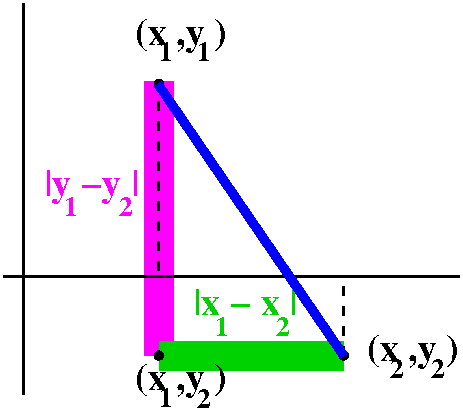 Distance in the plane, R2
Well, I went through the usual diagram to try to motivate the
algebraic definition of distance in R2. Look, please, at
the diagram to the right. In the plane, points correspond to ordered
pairs of numbers. So a point p might correspond to an ordered pair,
(x1,y1), and q might correspond to (x2,y2). Then the point (x1,y2) is
the vertex of a right triangle whose hypotenuse is a line segment
connecting p and q. One leg of the right triangle is on a line where
all the first coordinates are x1, and the length of that leg is given
by the one dimensional formula, |y1-y2|. The other leg is on the line
where all the second coordinates are y2, and the length of that leg is
|x1-x2|. Then by Pythagoras, the hypotenuse has length
sqrt(|x1-x2|2+|y1-y2|2). And usually the
absolute values are discarded since we are squaring the
quantities. Therefore we officially define:
dist(p,q)=sqrt((x1-x2)2+(y1-y2)2) if p
has coordinates (x1,y1) and q has coordinates (x2,y2).
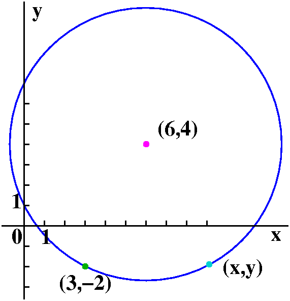
Example
The distance between between (3,-2) and (6,4) is
sqrt([3-6]2+[4-(-2)]2)=sqrt(32+22)=sqrt(13).
A circle and its algebraic description
Suppose we wanted to describe algebraically the collection of all
points which have distance sqrt(13) from (6,4). This is, of course, a
circle of radius sqrt(13) and center (6,4). Well, if (x,y) is such a
point, then sqrt([x-6]2+[y-4]2)=sqrt(13). This
does describe the circle. Of course, if you must, all sorts of
algebraic things could be done to the equation. But I am the laziest
person in the room, and therefore ...
A (non-vertical) line and its algebraic description
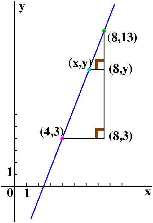 Suppose we wanted an algebraic description of points with coordinates
(x,y) which lie on the straight line which goes through (4,3) and
(8,13). If (x,y) is such a point, then look at the picture: two right
triangles indicated are similar, so the corresponding sides have the
same ratios:
13-y   13-3
---- = ----
 8-x    8-4
and the point (x,y) is on the line exactly when
y-13=([13-3]/[8-4])(x-8). The quantity ([13-3]/[8-4]) is called the
slope, and multiplies changes in x to give changes in y. It is
frequently designated with the letter m.
QotD
I gave two points and asked for an equation for the line containing
the two points. Most people were able to do this.
Maple
Much intricate algebraic computation can now be done by computer
programs. A course like Math 151 can therefore comcentrate more on
understanding rather than elaborate computational skills. On
the other hand, knowing what results should look like (if you
calculator declares that 56.007 is the sum of 1,345 and -14,891, do
you believe it?) is important, so a secure command of various
algebraic algorithms is still important. At Rutgers, the program Maple is widely available since there is a
university license for it. Students may also get copies under certain
circumstances.
Basic information about the program is here
and here
are some local help pages.
Read the text!
Please read the first few sections of chapter 1, as on the Math 151
syllabus.
Maintained by
greenfie@math.rutgers.edu and last modified 9/7/2006.
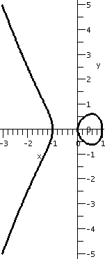
 The chain rule itself can be repeated. So here, for example,
we can try to differentiate cos(e3x2). Its
derivative is
-sin(e3x2)·(e3x2)·(6x).
I hope that you can pick apart the layers of the functions and their
compositions. One poor metaphor for using the chain rule is that it is
like peeling an onion very very carefully, layer by layer, and taking
care always of the outside most layer first. Confusion is certainly
possible, and that's an understatement. The "chain" in the chain rule
is, I think, a reference to the links (via composition) in a typical
algebraically described function.
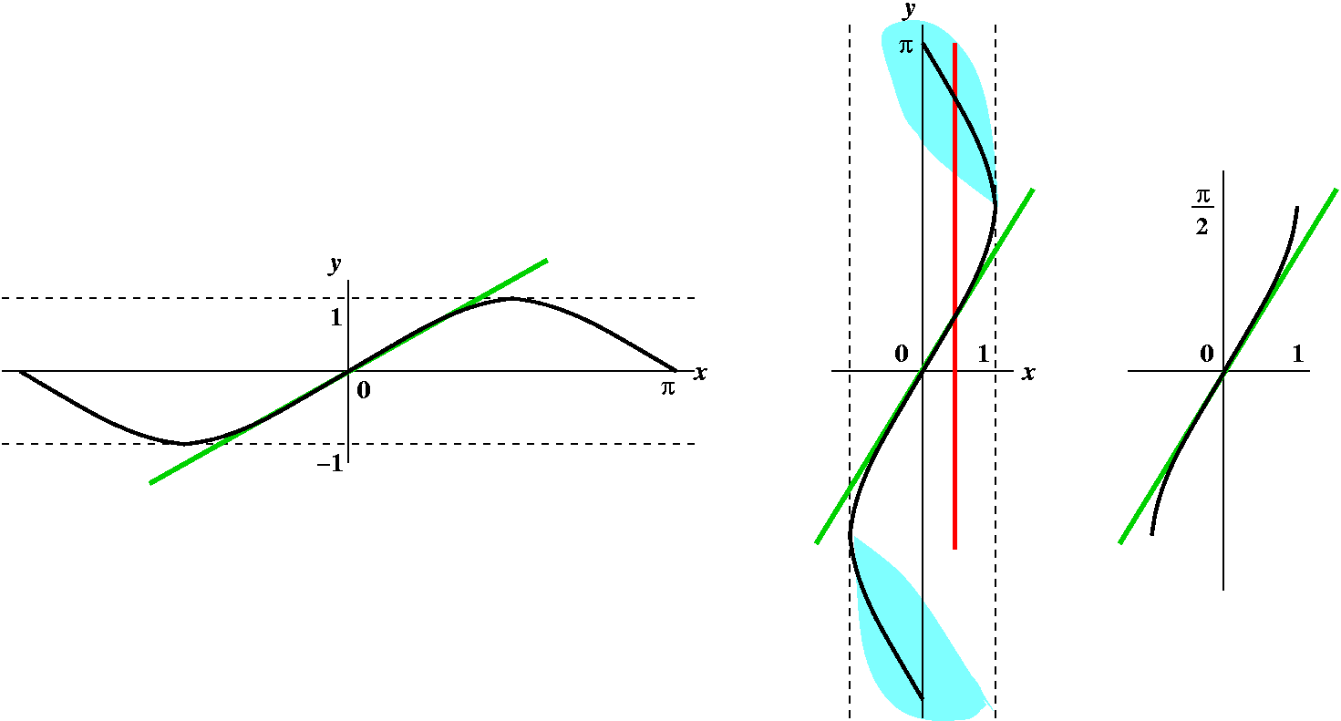
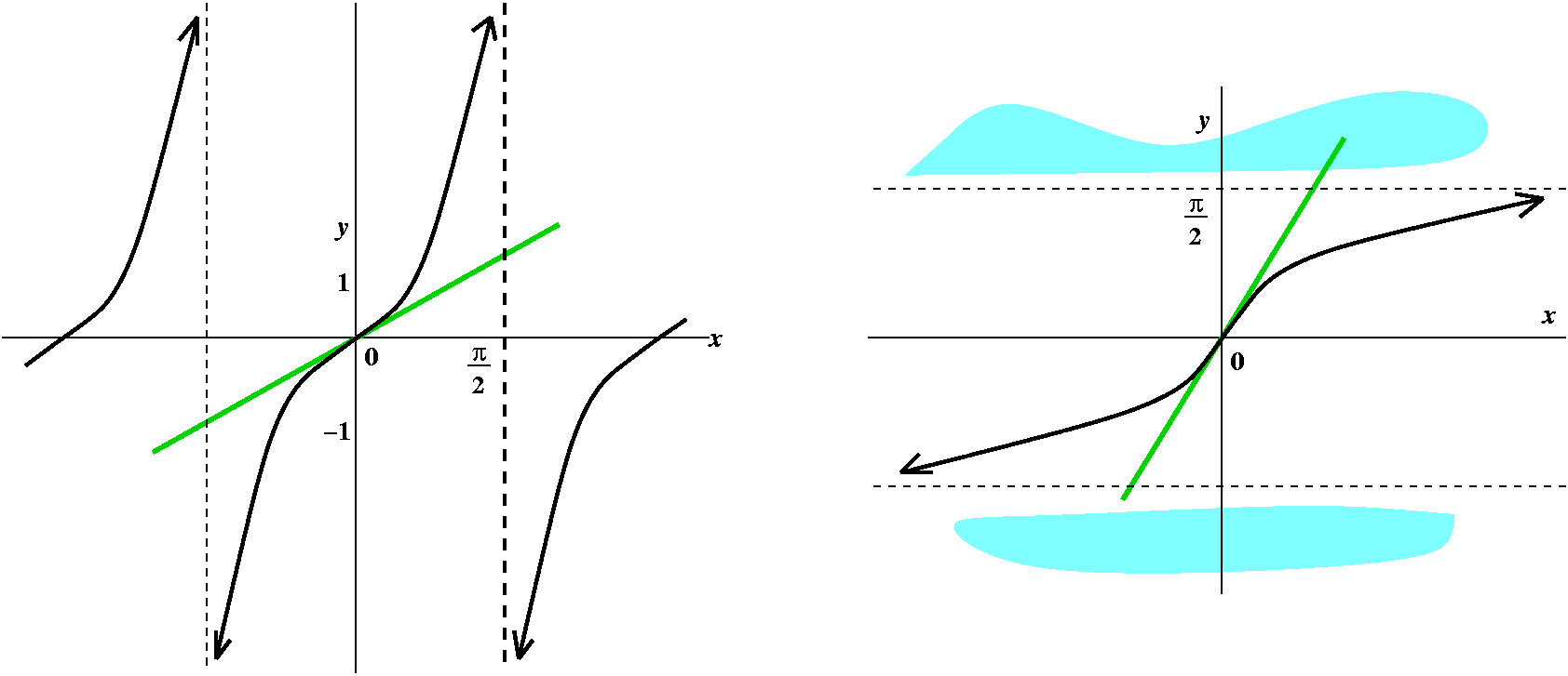
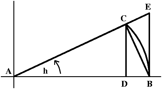
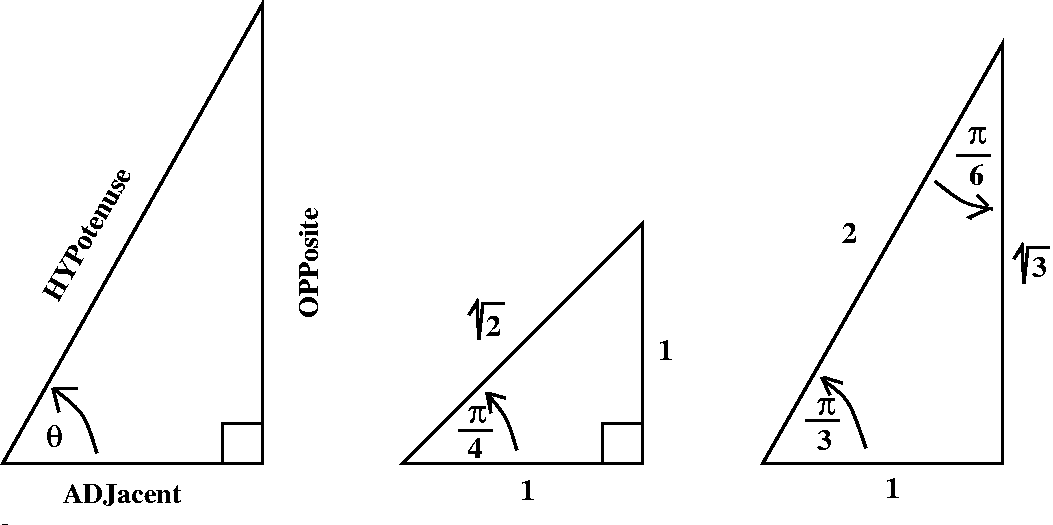 Here are the standard definitions of trig functions as related to
quotients of side lengths of right triangles:

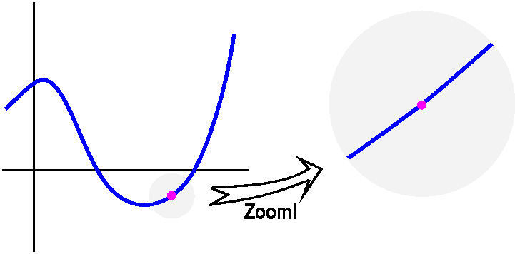
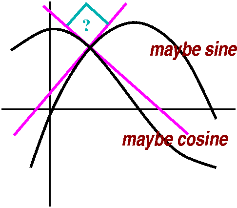 My final gasp was to draw a quick picture, the way we all do, of sine
and cosine. I distorted the bumps as almost everyone does. The bumps
are actually rather flat. But "clearly" the curves intersect, and,
look, look!, it seems that they intersect almost perpendicularly.
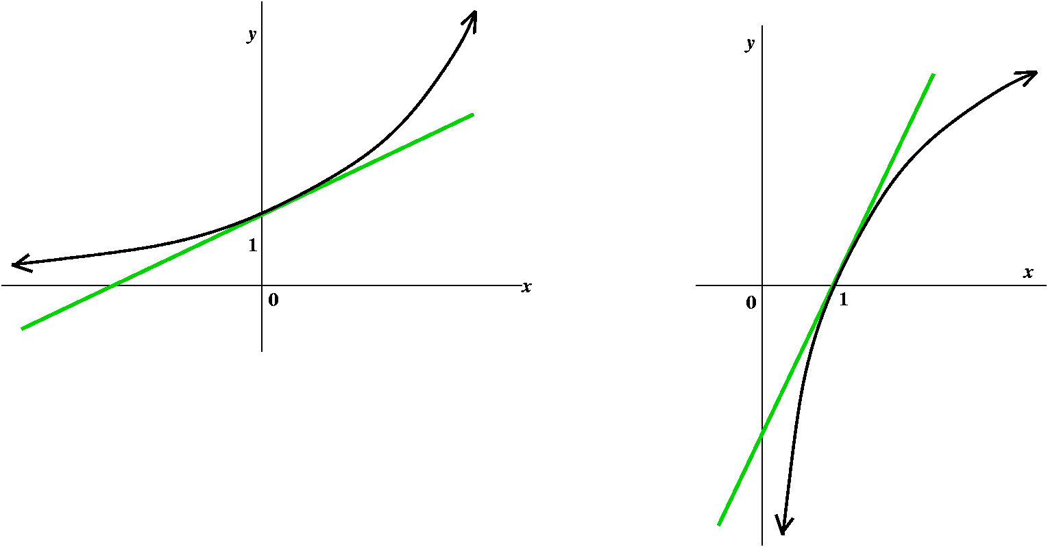
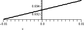
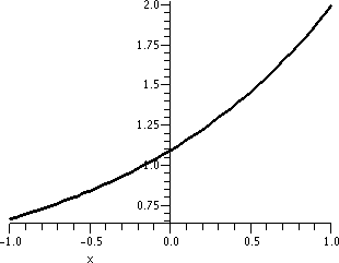
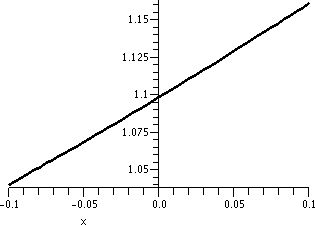
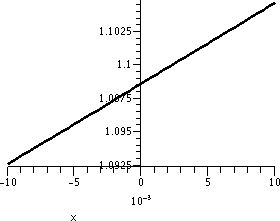
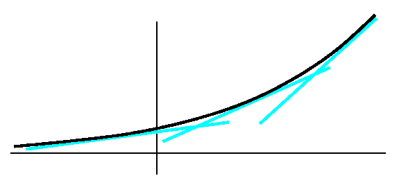 Your textbook next studies the exponential functions ax. If
a>1, this represents exponential growth. Consider the graph of an
"average" exponential growth function and the slope of the tangent
lines to this curve. As the point of tangency travels from left to
right, the slope, which is always positive, just increases. If we
could image a graph of the slope function (which is just a graph of
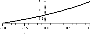
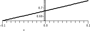
the function y=f´(x)) it might look a great deal like ax
itself. And that is the truth. A proof of this takes some
effort, and could be given now, but we are supposed to run as fast as
we can. So I will just write out some suggestive reasoning, following
more or less what is in your text. I'll also include some pictures,
mostly because pictures help me believe more.


 I needed 25 digit accuracy to get the last few entries in the first
row to 10 digit accuracy. Computations with small numbers which are
almost equal can be imprecise. But the numbers should help you
accept the previous results which were obtained with algebraic
manipulation.
 f(a+h)-f(a) is the difference in position at the two times
indicated. This is also called displacement. In general, this
is not the distance that the point travels between those two
times, because the moving point could wiggle back and forth.
 [f(a+h)-f(a)]/h is the slope of the secant line through the
points (a,f(a)) and (a+h,f(a+h)).
 If, as h-->0, the slope of the secant line approaches a
limit, this limit is called the slope of the tangent line to y=f(x)
at x=a.


 To the right is the graph of a function, f(x), whose
domain includes all x except for 3. The "arrows" at the top of the
curve are supposed to indicate that as x gets closer and closer to 3
(on either the right or the left side) then f(x) gets large. But
there's more, really. It doesn't just "get" large in some uncontrolled
way. The function is
supposed to
 sin(x)/x
 x/sqrt(x2+3)
 We discussed various curves which could represent the position of
Francine on the parkway in terms of miles from the start of the
parkway at time t, in terms of hours elapsed from 7 AM. I tried to
show that our everyday intuition lead to the graph being
increasing (as you travel from left to right, the points on
the graph go up). The graph can have level spots, where Francine pulls
over for a rest stop. Legally Francine isn't supposed to drive
backwards, though.


 Slope of a tangent line


 Possibly the slope of another tangent line




 Piecewise defined functions


 A piecewise linear function to play with


 Distance in the plane, R2
 Suppose we wanted an algebraic description of points with coordinates
(x,y) which lie on the straight line which goes through (4,3) and
(8,13). If (x,y) is such a point, then look at the picture: two right
triangles indicated are similar, so the corresponding sides have the
same ratios: