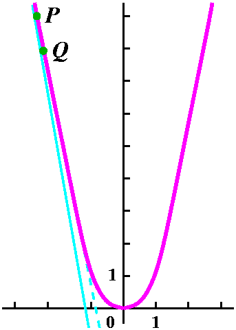
 The second example
What is the equation of the line tangent to y=x2 when x=-3?
What will we do?
I mentioned in class today that almost everyone who sees the material
we will begin to discuss today thinks that it is one of the high
points of human intellectual achievement. We surely have prepared for
this in earlier meetings of the course.
A useful quote?
The text in section 3.1 introduces the rate of change idea by
analyzing tangent lines to curves. "Students" are somehow intuitively
supposed to know what tangent lines look like. The quote I used in
class to emphasize this comes from U.S. Supreme Court
Justice Potter Stewart, who supposedly remarked about pornography, "I
cannot define it, but I know it when I see it." Analyzing tangent
lines is sort of like that. An exact definition is difficult, and you
are supposed to "know it" when you "see it."
My only quarrel is that I don't believe most students in the class
have majors where they will be interested in computing tangent
lines, so "tangent lines" themselves don't seem a rich source of
motivation.
The first example
What is the equation of the line tangent to y=x2 when x=1?
The equation of a line (let's suppose it is not vertical!) is y=mx+b. There are two constants, m and b. Geometric data which will yield m and b are generally in one of the following forms:
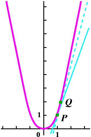 In the case of "the line tangent to y=x2 when x=1", I know
(because I know it when I see it!) that the line goes through the
point (1,12). I write the second coordinate as
12 and not just 1 because I want to emphasize that we got
it as a point on the graph of y=x2. We need to find a
slope, m. In fact, because it is the slope of the tangent line, I will
call it mtan.
Appoximating mtan by msec
The idea of this motivating example is containing in the picture to
the right. But please note that this picture has lots of information
implicit in it. The point I call P is supposed to be
(1,12). O.k.: it is (1,1). The point Q is
close to P: it has first coordinate 1+h. Therefore since Q is
on the graph of y=x2, the second coordinate of Q must be
(1+h)2. The line connecting P and Q is frequently called
a secant line (it is the dashed line in the picture) and you
are supposed to believe that this secant line has slope close to the
slope of the tangent line to y=x2 at (1,1,) when Q is close to P. That's the same as
asking that h be very small. I'll call the slope of this secant line
msec. What is msec algebraically? I can get this
from the points Q=(1+h,(1+h)2) and P=(1,1). So
msec=[(1+h)2-1]/[(1+h)-1]. It
would be nice to forget that right here in class the instructor made
an embarrassing algebraic error.
I am interested in what happens as h-->0. That is, what can we
say about limh-->0mh? Well, look at
[(1+h)2-1]/[(1+h)-1]. The bottom +1 and -1 cancel. So the
result is [(1+h)2-1]/h. If I try the "plug in" method to
see what happens, I get 0/0, which is bad. This is the model situation
for limits. In this case and in the others which I'll consider
today algebraic transformations (which I referred to in class as
algebraic massaging) will make the limit behavior clear.
So [(1+h)2-1]/h=[1+2h+h2-1]/h=[2h+h2]/h=2+h. Therefore limh-->0msec=limh-->02+h=2 and my "guess" for mtan is 2.
The answer
I now believe that the tangent line to y=x2 when x=1 goes
through the point (1,1) and has slope equal to 2. So the line is
(y-1)=2(x-1). Unless these is some reason or reward, I would probably
leave the answer this way (yes, I agree that I could write it as
y=2x-1 but why risk touching it since I might "break it": that is,
make some silly arithmetic error).
Comments
In this lecture and in the following lecture, I am interested in the
ideas. It turns out that for functions defined by simple
formulas, computing slopes of tangent lines is a nearly mechanical
process. Most of the examples of functions you will meet in the
real world will reveal themselves through graphical information or
numerical data. I doubt very much, for example, that a veterinarian
will learn that the usefulness of a canine tranquilizer is
4x2-9x+4. Much more likely ways of conveying what's know
would be a table of data or a graph. So please learn the ideas
right now.
 The second example
What is the equation of the line tangent to y=x2 when x=-3?
When x=-3, y=(-3)2=9. So I will put P at (-3,9). What about Q? Q will be located where x=-3+h, for some very small number h. The coordinates of Q, another point on the graph of y=x2, will be (-3+h,(-3+h)2). What information do I know about the line tangent to y=2 when x=3? I know the line passes through (-3,9), and that its slope, mtan, will be limh-->0msec where msec is the slope of the line through P and Q. I asked in class at this point in the exposition whether mtan could be 2, and I was told "Certainly not" because the sloe of the tangent line was "clearly" tilted down, so mtan should be negative.
Investigating msec
The coordinates of P and Q allow me to write a nice formula for
msec: [(-3+h)2-9]/[(-3+h)-(-3)]. First on the
bottom the -3's cancel. It is important to keep track of minus
signs. In my computations, when I'm working by myself, I sometimes
tend to lose track of them. But that's a terrible idea here, since
various cancellations are important. So msec=[(-3+h)2-9]/h.
As h-->0, if I try to "plug in" I get the unacceptable 0/0 again. Some algebra:
(-3+h)2-9   (-3)2-6h+h2-9   9-6h+h2-9   -6h+h2
--------- = ------------ = --------- = ------ = -6+h
    h             h            h         h
These algebraic transformations are all valid when h is not 0.
Therefore (as we say in math courses),
limh-->0msec=limh-->0-6+h=-6 and this
must be mtan.
The answer
I now believe that the tangent line to y=x2 when x=-3 goes
through the point (-3,9) and has slope equal to -6. The slope is
negative, even as predicted earlier from the picture. So the line is
(y-9)=-6(x-(-3)).
The third example
What is the slope of the line tangent to y=x2 when
x=x0?
I concentrate my attention on the slope because that's really the
interesting information.
Now the algebra will be more intense and I will also make the
situation more "interesting" by skipping a few steps. The point P has
first corrdinate x0 and is on y=x2 so it is
(x0,(x0)2). The point Q has first
coordinate x0+h where h is some small (but non-zero!)
number. Since Q is also on the curve y=x2, its coordinates
are
(x0+h,(x0+h)2). Now msec
is [(x0+h)2-(x0)2]/h. Here
I've already cancelled +x0 and -x0 from the
bottom of the fraction. You must practice this, please! Here we
go:
(x0+h)2-(x0)2   (x0)2+2x0h+h2-(x0)2    2x0h+h2
------------ = ------------------- = ------- = 2x0+h
      h                  h              h
which is valid when h is
not 0. Therefore
The answer
The slope of the line tangent to y=x2 when
x=x0 is 2x0.
Comments
I urged students to realize that when x0<0, the slope of
the tangent line was negative. Hey: the tangent lines and the curve
are both decreasing as we walk from left to right. Of course, when
x0>0, the reverse occurs. The tangent lines and the
curve both go up (increase) as we walk from left to right.
Of course, this discussion is about a simple function and simple
graph. But the ideas will work in situations which are much more
complicated.
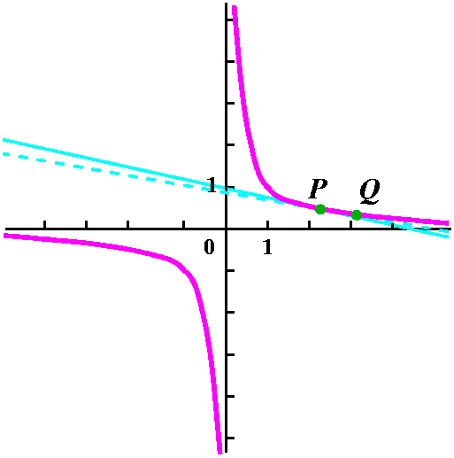 A hyperbola example
y=1/x is a hyperbola. What is the slope of the line tangent to y=1/x
when x=x0?
We looked at the graph of y=1/x and immediately (well, fairly soon)
recognized that the slope of the tangent line would always be
negative. This is sort of weird but true, and will allow us to check
the result we get, at least roughly. O.k, now to work. Here is what I
will mumble to myself:
P ... Q ... x0 ... 1/x0 ... x0+h
... 1/[x0+h] ... msec ...
The picture may not be that helpful. I am sorry.
You are not allowed to make algebraic errors in what
follows. So:
   1      1        x0-[x0+h]         -h
 ----  - ---     ------------      --------
 x0+h     x0        [x0+h]x0        [x0+h]x0     -h
------------- = -------------- = ---------- = ---------
     h                h                h      h[x0+h]x0
And now, since today only I am trying to be careful, I note that
since h is not 0, this is the same as
-1/[x0+h]x0. If h-->0, then
this-->-1/[x0]2. This is the slope of the
tangent line. I'll note again that your algebra needs to be
really clean, neat, and correct, otherwise you will have little chance
of getting the right answer.
Cheap check
Yes, the slope of the tangent line is
-1/[x0]2
and this is always negative for all
x0 in the domain of f(x)=1/x (that is, when x0
is not 0).
A hyperbola subexample
What is the equation of a line tangent to y=1/x when x=7?
Well, when x=7, f(7)=1/7. The tangent line passes through (7,1/7). The
slope of the tangent line is gotten by substituting x0=7 in
the formula -1/[x0]2 so the slope is
-1/(49). Here is the answer as I would write it:
(y-(1/7))=[-1/(49)](x-7).
Definition of derivative
f(x) is said to be differentiable at x0 if
limh-->0[f(x0+h)-f(x0]/h exists. If
this limit exists, then the value of the limit is called the
derivative of f(x) at x0. The usual notation for this limit
is f´(x0).
The future and the far future ...
The QotD last time
Is there a number x so that 2x+3x=4x?
Give evidence supporting your answer.
Possible answers:
|  |
|  | ||||||||
| Exponential rules | Log rules | AB+C=AB·AC (AB)C=ABC A0=1 A-B=1/AB |
logAB=C means B=AC logA(B·C)=logAB+logAC C·logAB=logABC logA1/B=-logAB logA1=0 |
|---|
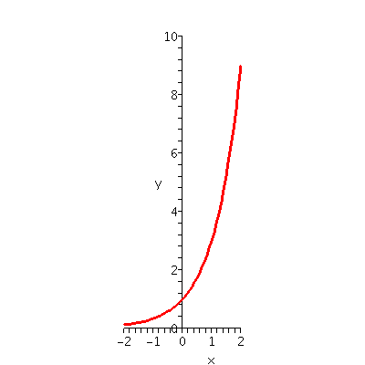
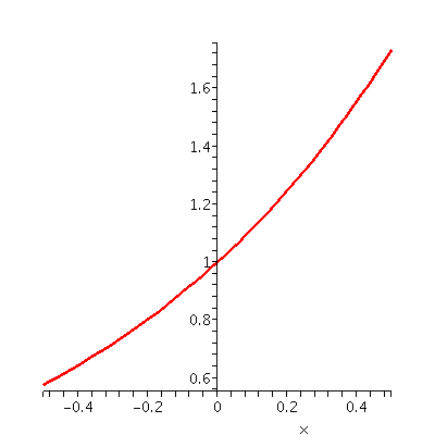
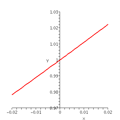
Here I began by asking people to use their graphing calculators to draw y=3x, and then start zooming in. Three views are shown below:
| y=3x for x in [-2,2] | y=3x for x in [-.5,.5] | y=3x for x in [-.02,.02] |
|---|---|---|
 |
 |
 |
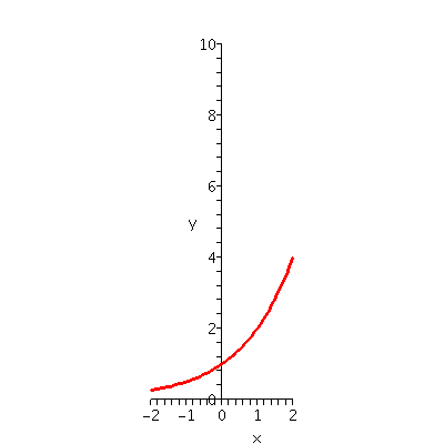
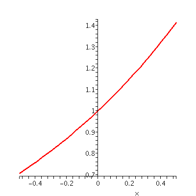
Now I asked people to do the same for y=2x. Here are some results.
| y=2x for x in [-2,2] | y=2x for x in [-.5,.5] | y=2x for x in [-.02,.02] |
|---|---|---|
 |
 |
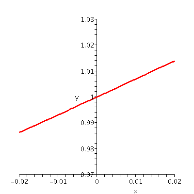 |
 The
large-scale qualitative aspects of y=2x are very similar to
those of y=3x. Now we zoom in, and the curve seems to
flatten out. The slope of the resulting (almost) line is about
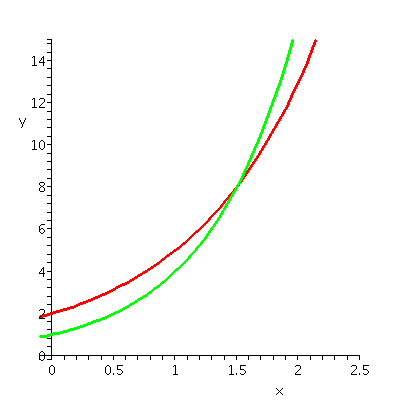
.693. Indeed, we could try to graph y=2x
(the green curve) and y=3x (the red
curve) together, as shown to the right. You can see that both
curves go through (0,1), and that the local growth rate (o.k., the
"slope") of the red curve is greater than that of the green curve. We
will be doing a great deal of computation of growth rates. If we
had to constantly work with .693 and 1.089 these computations
would be more tedious.
So what people use who do lots of computations with rates is to find a
positive number A so that the "local rate" of y=Ax near
(0,1) will be 1. So we will look for an A so that
limx-->0[Ax-1]/x will be 1. This number will be
something between 2 and 3, because 3x tilts too much
(1.089) and 2x tilts too little (.693)
"This porridge is too hot!" she exclaimed.
So, she tasted the porridge from the second bowl.
"This porridge is too cold," she said.
So, she tasted the last bowl of porridge.
"Ahhh, this porridge is just right," she said happily and she ate it all up.
The textbook suggests taking small x's (that would appear in the
limx-->0 idea) as 1/n, where n is a large positive integer.
Then [A1/n-1]/(1/n) will be close to 1 when n is large.
We can unroll this and get [A1/n-1] will be close to 1/n
when n is large, and further unroll so that
A1/n will be close to 1+(1/n). Hey, now take nth
powers (all of this is not obvious but has lots of cleverness
built in). Therefore the candidate for A will be approximately
(1+(1/n))n.
Here is a table somewhat more complete than what I wrote in class.
| n | 10 | 20 | 30 | 40 | 50 | 100 | 250 | 500 | 1,000 |
|---|---|---|---|---|---|---|---|---|---|
| (1+(1/n))n | 2.59374 | 2.65329 | 2.67431 | 2.68506 | 2.69158 | 2.70481 | 2.71268 | 2.71556 | 2.71692 |
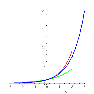 It turns out that there is exactly one number, usually called
e, so that y=ex has local growth rate equal to 1 at
(0,1). This number is the one which we (and virtually everyone else in
the world who analyzes growth and its decreasing counterpart, decay)
will use. To the right is displayed y=ex, "sandwiched" by smaller
pieces of the curves y=2x
and y=3x. The number e is
approximately 2.71828 (I am willing to bet that you will never
need to know a more accurate approximation, but if you do, here is
one: 2.71828182845904523536028747135.)
Financial stuff
The textbook has information about compounding interest and what's
called continuous compounding. The relevant formulas are on the
top of page 89.
My sloppy lab notebook
I could imagine that I am observing a colony of bugs, and I will
assume that the number of bugs in the colony increases
exponentially. Such assumptions are sometimes correct for short
periods of time, and reflect the biological idea that the rate of
increase of the population is directly proportional to the population
(if more bugs, then more bugs are born). So here is a section of my
lab notebook.
| Time | Number of bugs observed |
|---|---|
| 9 AM | 23 |
| 10 AM | Cocoa stain!!!! |
| 11 AM | 121 |
| Lunch mess!! | 188 |
Can we reconstruct the data that's been lost? Under the initial
assumption, the answer is yes. If we assume that B(t), the number of
bugs at time t, is Cer t, for C and r "unknown"
constants, then what do we know? First, I will clarify things a bit,
and measure t in hours starting from 9 AM. Thus B(0)=23. But since
B(t)=Cer t, I know that B(0)=C (since
e0=1). Therefore B(t)=23er t. But we also
know that at 11 AM there are supposed to be 121 bugs. So B(2)=121, and
in terms of the assumed formula, 23er 2=121. Now
"solve" for r:
er 2=121/23
Take "logs"
(actually, in terms of the way your book is written, we should take
"lns", natural logs, which are logs using the base e):
r 2=ln(121/23).
So r=(1/2)ln(121/23) which my calculator
tells me is approximately .830148.
Now I have a "mathematical
model" for my bug population:
B(t)=23e.830148 t
Under
the cocoa stain is
B(1)=23e.830148 1, which is about 52.75.
What time was lunch? We need to solve
188=23e.830148 t, and this gives
188/23=e.830148 t and then ln(188/23)=.830148 t
so that t=[1/(.830148)]ln(188/23) which is approximately 2.5308, so
lunch was slightly after 11:30.
QotD
Is there a number x so that 2x+3x=4x?
Give evidence supporting your answer. This evidence could be numeric,
or graphical, or even quoting some theoretical result of the
course, but I'd like some evidence.
Decay
I did not have enough time in class to discuss typical decay
curves. These are y=Ax where 0<A<1. They are related
geometrically to growth by reflection across the vertical axis. For
example, y=(1/2)x has the point (5,1/32) on it, and on
y=2x the corresponding point is (-5,1/32) (I'm using
A-B=1/AB.) Notice that
(1/2)x=2-x. So flip all the growth curves to get
decay curves. Decay curves also use only the top half of the plane,
and they decrease to 0 as x-->infinity.
HOMEWORK
Finish reading the parts of chapter 2 we need, and please do some
homework problems.
Section 2.2, #23
What is limx-->0[sin(2x)]/x? Here is how I thought about
this problem. I
wrote:
sin(2x)      sin(2x)      sin(2x)
------- = ------------ = --------· 2
  x         2x (1/2)        2x
Therefore limx-->0[sin(2x)]/x=limx-->0{[sin(2x)]/(2x)}·2=1·2=2. My efforts were entirely trying to get 2x "underneath" sin(2x) as x-->0, because then I could apply the logic of sin(something small) divided by the same something small is fairly near 1." The result gives me a 2 upstairs, and this turns out to be the result of the limit computation.
Section 2.2, #25
What is limt-->0[tan(5t)]/[tan(2t)]? Again, let me show
you how I tried to think through this problem.
 [tan(5t)]     [sin(5t)/cos(5t)]      sin(5t)·cos(2t)
----------- = -------------------- = -----------------
 [tan(2t)]     [sin(2t)/cos(2t)]      sin(2t)·cos(5t)
The first algebraic "thing" I did was motivated by my intense personal dislike of compound fractions. I find them complicated and sometimes difficult to understand. Of course, it is possible to make errors when changing the compound fractions into simple fractions, so some alertness is needed. Now here is what I did with the simple fraction:
 sin(5t)·cos(2t)     sin(5t)     cos(2t)       1
----------------- = --------- · --------- · --------
 sin(2t)·cos(5t)        1        cos(5t)     sin(2t)
Now what? Well, I have a picture of cosine installed in my brain, and therefore I know that cos(some small number) is close to 1. So I don't need to think too much about cos(2t) and cos(5t) as t-->0. But I want 5t underneath sin(5t) and 2t over sin(2t). When I put them in, I need to compensate:
 sin(5t)     cos(2t)       1         5  sin(5t)  cos(2t)      2t
--------- · --------- · --------- = --- -------- --------- ---------
    1        cos(5t)     sin(2t)     2    5t      cos(5t)   sin(2t)
Now I can analyze the limit. The first chunk (o.k., more properly,
the first quotient) gives me 5/2. The next is a sine of a small number
divided by the same small number, which gives me 1.
And the cosines just give me 1. And the last quotient also gives me
1. So I bet that
limt-->0[tan(5t)]/[tan(2t)] will be 5/2. A function is continuous if its graph has no jumps or breaks. For example, the crazy numbers in the U.S. tax table (Schedule X) occurred because as a consequence of public policy, the tax function should be continuous, and the graph should not have any breaks or jumps.
I asked the following question:
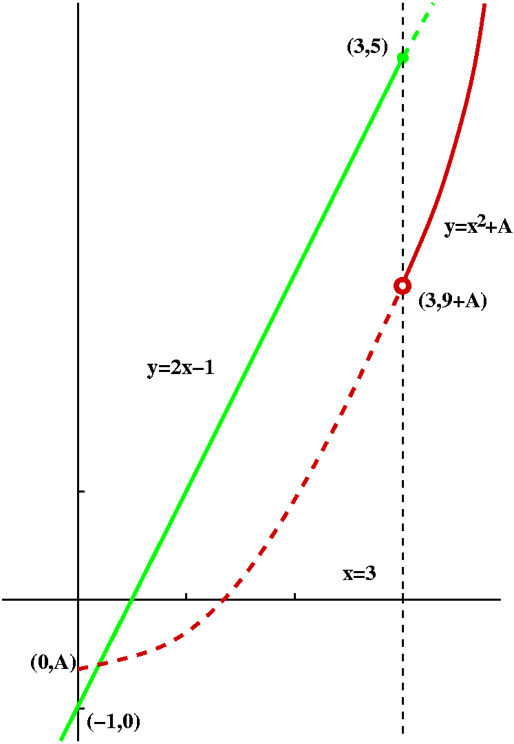 Suppose f(x) is defined piecewise by
     { 2x-1 for x<=3
f(x)={
     { x2+A for x>3
Can we find a value of A for which f(x) is continuous at x=3?
First I wanted to graph this function, since I, at least, think better when I have a picture to reason with. When x<3, f(x)=2x-1 and this is part of a straight line whose slope is 2 and whose y-intercept is -1. I just need the half-line which is to the left of x=3.
To the right of x=3, we need to think about f(x)=x2+A. Of course, y=x2+A is a parabola whose axis of symmetry is the y-axis. Its "vertex" (lowest point, the parabola opens up) is at (0,A). The graph of y=f(x) for this f(x) takes only the part of this parabola which is to the right of x=3.
The left-hand limit of f(x) at x=3 uses 2x-1, and the value of this limit is 2·3-1=5. This is also equal to the value of f(3). The right-hand limit uses x2+A, and as x-->3-, x2+A-->9+A. To make all three of these coincide (5 and 9+A and the "other" 5) we need just to choose A=-4. So this function will be continuous at x=3 exactly when A is chosen to be -4.
 The last QotD
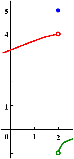
I asked for the graph of a function with the properties that
Precise definition of continuous for Math 135
A function f(x) is continuous at x=a if
limx-->af(x) exists and equals f(a).
This means that limits for continuous functions can be evaluated just
by "plugging in", so these functions are nice and tame. There is one
really important theoretical consequence of continuity
which almost everyone uses unconsciously. Let me lead up to this
result (the Intermediate Value Theorem) by describing driving on one
of New Jersey's jewels.
The Garden State Parkway, from Cape May to Montvale
and my friend Francine ...
I then discussed the Garden State Parkway. We spent quite a lot of
time on the question of the
length of the parkway. Mile 0 is at Cape May, while the other
end, mile 172, seems to be close to Montvale.
Suppose that my friend Francine leaves Cape May at 7 AM one morning,
and drives north on the Garden State Parkway. Further, suppose she
arrives at mile 172, the northern end, at, say, 10 AM. Must Francine
at some time be at mile 135 (fairly near Busch campus)? The parkway
seal below was "borrowed" from a State of New Jersey webpage.
I discussed various curves which could represent the position of Francine on the parkway in terms of miles from the start of the parkway at time t, in terms of hours elapsed from 7 AM. I tried to show that our everyday intuition lead to the graph being increasing (as you travel from left to right, the points on the graph go up). The graph can have level spots, where Francine pulls over for a rest stop. Legally Francine isn't supposed to drive backwards, though.
If we believe that motion is continuous (so Francine does not have a Star Trek transporter or other device) then the graph of Francine's position goes from (7 AM, 0 miles) to (10 AM, 172 miles) and therefore the graph must have on it at least one point with coordinate description (*,135). All of this, by the way, rests on some complicated assumptions, some of them philosophical (why should motion be continuous?). Today, though, I believe that motion is continuous, and therefore at sometime Francine must be at Mile 135. By the way, I will retain this information for later, when we analyze the rate of change of position (velocity) so that we can see whether Francine deserves a speeding ticket.
The Intermediate Value Theorem
Suppose that the function f is
defined and continuous on the interval [a,b]. Then the equation f(x)=y
has at least one solution for every y which is between f(a) and f(b).
Math 135 example for the Intermediate Value Theorem
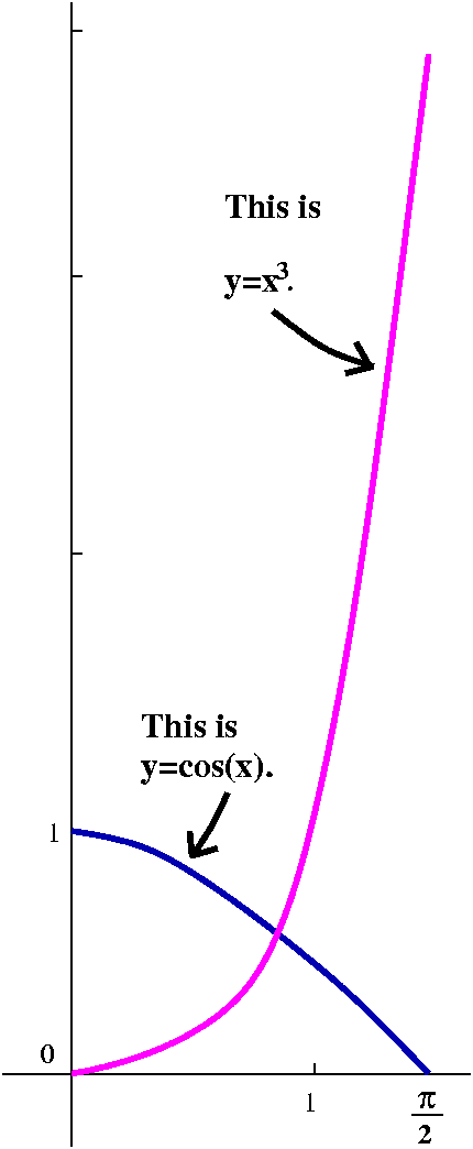
Look at cos(x) and x+x3 on [0,Pi/2]. I claim that there's a
number x in the interval from 0 to Pi/2 where
cos(x)=x3.
I tried to analyze this first by showing you what I had in mind when I thought initially about this problem. Well, Pi/2 is approximately 1.57, and (1.57)3 is approximately 3.86 or so (yes, I used an electronic friend for this). So if you look at the picture, you should see that the curves cross. Hey! Wow!!
Now to give the answer that Math 135 will recognize. Consider the function f(x)=cos(x)-x3. Then f(0)=cos(0)-03=1 which is a positive number, and f(Pi/2)=cos(Pi/2)-[Pi/2]3=0-[Pi/2]3, and this is a negative number. The functions involved (x3 and cos(x)) are both continuous. Then the Intermediate Value Theorem applies to this function f(x) and the interval [0,Pi/2], and shows that there exists at least one number x with f(x)=0. But f(x)=0 means cos(x)-x3=0 which means in turn that cos(x)=x3.
Comment This is what is known as an "existence result". I don't think anyone would feel that the root has really been discovered or approximated in any meaningful way by what we've done here. In fact, though, exactly such ideas are used by your hand calculator to find approximate solutions to equations. The calculator first "looks" for where the graphs cross each other, and then the calculator tries to sort of "localize", and get better and better approximations to the roots. The sort of approximation works well in a surprising variety of examples. The number x=.8654740331 comes out as an approximate root of cos(x)=x3 very rapidly from a machine.
QotD
Try to explain why the equation tan(x)=x must have
positive solutions.
HOMEWORK
Please continue to read chapter 2. Please hand in these problems at
Thursday's recitation:
2.2: 14, 18, 24, 43
2.3: 12, 19, 28, 43
|
lim f(x) = L x-->a |
We looked at a complicated, ferocious, horrible limit, and a nice baby lamb limit.
One example
What is the limit as x-->0 of
sqrt{45x34+
[1/sqrt{20x14+16}]+57x88
}?
This might look like a ferocious limit to people. I would try not to
get excited or anxious, and instead "parse" this expression
systematically. When x-->0 (which I read internally as "x gets close
to 0"), I look at, say, 45x34. In spite of the decorations
(?) of 45 and 34, this is really a simple and reasonable function. As
x gets close to 0, I think that the 34th power of x gets
close to 0. And multiplying this by 45 doesn't change that situation
much. So this piece of the "ferocious function" just -->0. The same is
true about 57x88. But what about
1/sqrt{20x14+16}? Well, one piece of this is
20x14 which also -->0. In fact, this bewildering (?) limit
is mostly just decoration: all the pieces -->0 except for the 16 which
is internal to two square roots and one reciprocal. Hey: I bet that
the limit exists, and that its value is sqrt{1/[sqrt(16)]}. By the
way, I would be happy with this sort of answer on an exam. If you must
"simplify", I guess another valid form of the answer is 1/2.
Another example
What's the limit as x-->0 of x/|x|? This is supposed to be the "baby
lamb" limit, I guess, because it such minimal typography. In fact, to
me this limit is much more complicated than the previous one. The
absolute value signs indicate that, to be really sure of the result,
I'd better analyze this limit in a piecewise fashion. So if x>0, I
know that |x|=x, and then x/|x| is 1. If x<0, then |x|=-x, and
x/|x|=x/{-x}=-1. So I hope you have a picture in your head of the
graph of x/|x|. It is -1 to the left of 0 and +1 to the right of
0. The notation "x-->0" is supposed to indicate no bias between left
and right: both sides should go to the same limit. Here that is
certainly not the case. The left-hand limit is -1 and the
right-hand limit is +1. Therefore the standard (two-sided) limit
does not exist. This "baby lamb" limit is actually much more
badly behaved than the first example, in some really profound sense.
The notation "limx-->a" denotes a two-sided limit.
If we wanted a left-handed limit, what's usually written is
limx-->a- and if we wanted a right-handed limit,
the notation limx-->a+ is used.
So limx-->0-x/|x|=-1 and
So limx-->0+x/|x|=1.
The two-sided limit exists when both one-sided limits exist and when
they agree. There are more examples in your textbook.
I think I tried one more example, something like, "What is the limit
of x+{|x-2|/(2-x)} as x-->-2-?" First, the notation is
somewhat confusing if you are new to this game, since "-2-"
has two minus signs. The minus sign in front of 2 indicates a negative
number, two units to the left of 0. The minus sign up in the corner
shows that I want to approach -2 from the left. So what can I do? If
x-->-2-, then x<2, and what can we say about x-2 itself?
Since x<2, x-2<0, so x-2 is negative and |x-2| is -(x-2).
Therefore x+{|x-2|/(2-x)} becomes x+{-(x-2)/(2-x)}=x+(-1(-1))=x+1, and
as x-->-2-, x+1-->-2+1=-1. The left-hand limit of
x+{|x-2|/(2-x)} at -2 is -1.
You can check that x-->-2+ the limit of x+{|x-2|/(2-x)} is
+1.
Serious note I've done lots of these computations. Even when I
am alone, I tend to use the inequality approach that I showed above. I
know that I can guess, and I know that my guess will
frequently be correct. But I've learned that sometimes my guesses will
not be correct, and this can be irritating.
The actual definition of limit is on the bottom of page 56 of your text. I won't discuss the definition here, but I should mention that the definition is quite precise, and the definition was arrived at after probably a century of controversy about "What is (or should be!) a limit?" People made many mistakes, and a precise definition was adapted so that fewer mistakes and misunderstandings would occur.
Section 2.2 of the text (page 61 and what follows) discuss a number of algebraic properties of limits (the limit of a sum, the limit of a product, etc.). You should read through these and use them. These rules are exactly what I used to "tame" and evaluate the initial ferocious limit in this lecture.
The QotD yesterday provides an example of how algebraic manipulation can be used. I asked people to consider
1   1
- - -
x   2
-----
(x-2)
as x-->2. If you try what I always try first ("plug in") the result is 0/0, which is at best equivocal (I don't know what the heck it means). We could also try graphing this mess. Or we could try some simple algebra:
1   1      2-x
- - -    ------
x   2     (2x)        (2-x)       -1
----- = -------- = ---------- = ------
(x-2)    (x-2)      (2x)(x-2)    (2x)
There are several comments to make about the stages in this algebraic process. First, I dislike "compound fractions" and I almost always try to get rid of them. That's why I "pushed together" the two pieces in the top of the original fraction. Then I needed to know how to change the compound fraction (two ------'s) into a simple fraction (one -------). I did that, carefully. The last step is one which is logically a bit perilous. If x is not equal to 2 (so x-2 is not 0) then I can divide the top and bottom of the fraction by x-2. I need to be careful, and I will get a minus sign on the top. But I remember that that phrase "x-->2" means "x is close to 2 but x is not equal to 2". So the original
1   1
- - -
x   2
-----
(x-2)
is actually (away from 2!) equal to
  -1
------
 (2x)
. The second form is easy to understand as x-->2: it must get close to -1/4. Therefore the limit exists and its value is -1/4.
There are a few common algebraic tricks. If you practice with the textbook homework problems and with WeBWorK, you will be in good shape for what we need to do with this course.
A function you know all about
Suppose I call S(x) the squaring function. So S(x) is defined by
S(x)=x2. I think you know this function well, and you know
what its graph looks like (a parabola with "vertex" at the origin,
opening up, symmetric with respect to the vertical axis). Certainly we
know limits involving S(x). So I know that
limx-->2S(x)=4 and limx-->5S(x)=25
and limx-->-3S(x)=9.
A mild change
What if I changed one value of S(x)? That is, let me define the
function T(x) by the following piecewise statement:
     {x2 for x not equal to 7
T(x)={
     {-4 if x=7
So now T(2)=4 certainly and T(5)=25 certainly, and, with this silly
definition, T(7)=-4.
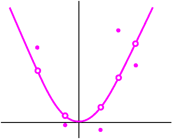 Aliens invade earth and change the squaring function!
Suppose that aliens invaded the earth, and took the function
S(x)=x2 and changed ten billion values of S(x). That is,
they created a new function, let me call it V(x), so V(x) has
the graph of S(x) except that ten billion of the points on the graph
have been moved, some up, some down. The domain of the function V(x)
is still "all real numbers" and V(x) squares all of the undisturbed
points of its domain. Otherwise V(x) does something alien. What do we
know about the limit of V(x) at, say, x=1? That is, what can we say
about limx-->1V(x)? One thing you don't need to worry about
is V(1). V's value at x=1 may have been changed by the aliens, but the
existence and value of the limit itself does not depend on V(1). So
don't worry about it. What happens as x-->1? Well, we might pass some
values of S(x) which have been changed by the aliens. For example,
between x=1.1 and x=1.01 we might pass by, say, a few million of these
changed values. Then between x=1.01 and x=1.001 we might go by some
more. Etc. But the aliens only changed ten billion or so
values, and eventually we will "pass" them all. There is infinitely
much room to the right and to the left of x=1. There are only finitely
many values which were changed. Eventually we get close enough to x=1
so that there are no more changes to be observed, and V(x) is the
"old" S(x)=x2 there. Hey: this means that
limx-->1V(x) exists, and is the same as
limx-->1S(x), and this limit is 12.
In fact, the same logic works at any point! limx-->wV(x)
will always exist, and it will always be the same as
limx-->wS(x)=w2. You may need to think this
through quite a bit. I can change the graph of S(x)=x2 in
any finite number of places, and I won't change the limits at
all! In order to change limits, I need to change an infinite amount of
data, which is quite different.
QotD Draw me a graph of a function with the following
properties:
The domain of f(x) is all real numbers, f(2)=5,
limx-->2+f(x)=4, and
limx-->2-f(x)=-1.
I did some problems in the textbook. Let's see if I can remember:
#5
What is
      z2+z-3
 lim --------
z-->1   z+1
Here I can just "plug in". There are no divisions by 0 to worry
about. The answer is -1/2.
        4-u2
 lim  --------
u-->-2  2+u
Of course here the top can be factored, and we get (2-u)(2+u) so that,
away from where 2+u is 0 (so u should not be equal to
-2) we can divide top and bottom by 2+u and we get 2-u as the result.
Now as u-->-2, 2-u-->4. So the limit exists and its value is 4.
Limits and inequalities
This was not well done in class. I rushed too much. I regret
the rush. Covering lots of stuff rapidly is much worse than doing a
few things well.
|
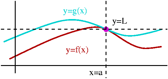
f(x)<=g(x) If I know that f(x)<=g(x) for all (relevant) values of x, and if I know that the limits exist, then limx-->af(x)<=limx-->ag(x). I think a picture supplies some substantiation, but I'll need to use this later in the course, and will return to it then. |
|
|
I also will need the Squeeze Theorem. f(x)<=g(x)<h(x) The logic is what is important. The hypotheses include the following: then limx-->ag(x), the middle limit, exists and equals the common values of the other two limits. Here the top and bottom functions are usually going to be something nice, and the middle function will be something weird. |
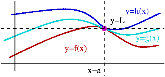
|
This early in the course the major use of the Squeeze Theorem is to analyze how sin(h)/h "looks" when h is a very small number. If you have a picture of sine then you know that sin(h) as h-->0 goes to 0. So sin(h)/h is definitely a "0/0" situation, and it is therefore one whose behavior can't be predicted, and whose limiting value, even if we assume the limit exists!, can't be predicted. Please believe me when I declare that sin(h)/h is an important 0/0 situation.
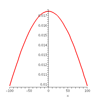
I did not use the Squeeze Theorem. For that, please see pages 67-68 of the text. I asked students whose last names began with the first half of the alphabet to use their graphing calculators to sketch sin(h)/h with radians, and I asked the students in the second half of the alphabet to sketch sin(h)/h in degree mode.
| Degrees: the "top" is about .01745 | Radians: the "top" is exactly at 1 |
|---|---|
 |
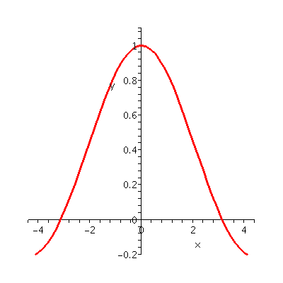 |
| This is part of the graph of sin(h)/h where I have forced the graphing program to evaluate sine in degrees. Look closely, please, at what happens as h-->0. The values of the function seem to be around .01745, and indeed, if you insist upon working with sine in degrees, the limit will be that rather unpleasant number. | Here is a picture of sin(h)/h where h is measured in what turns out to be much more natural units, "radians". The word is funny, but it just means the length of a piece of circular arc whose radius is 1 and whose angle is designated. This is a sort of "native" measurement, and you should please consult the textbook for a picture explaining why sine of a very small angle in radians is quite close to that angle itself. This is very neat, and very nice to use in practice. |
In this course I would rather cope with 1 than with .01745, so we will always use radian measure in calcuous applications.
|
Exercise E Consider E(x), which is defined by E(x)=1/K(x), where K(x) was my pet function.
BEGIN: PEDAGOGICAL RANT | ||
|
We have some precise information about K(x) in terms of four specific
points on its graph. I'd first try to exploit this precise information
as well as I could. For example, we know that K(1)=2 since (1,2) is on
the graph. Therefore, E(1)=1/K(1)=1/2, so that (1,1/2) is on the graph
of E(x). Also K(2)=4, so E(2)=1/K(2)=1/4, and (2,1/4) is on the graph
of E(x). Let me pause here, and ask if we can infer more information
for x's between 1 and 2. If I understand what the graph indicates, I
think that K(x) gets bigger (the "technical" word, I guess, is
increases) as x moves from 1 to 2. I know, darn it, that the
idea of x moving is silly (what the heck, there's the graph,
what is "moving" about that picture?). But I do think that way, and I
find it useful sometimes, and maybe you might also. So x goes from 1
to 2, and y, on the graph of K(x), goes from 2 to 4. What about 1/y?
When y is positive, 1/y, the reciprocal of y, is also positive. As y
increases, 1/y decreases. So the "chunk" of the graph of
E(x) for x between 1 and 2 decreases from 1/2 to 1/4.
Now the nice precise piece of information: E(3). Well, E(3)=1/K(3)=1/0 ALARM!. We don't divide by 0 in Math 135. In fact, here is the initial segment of
These manners must be minded when we worry about the domains of complicated algebraic functions. That won't often be the object of the game, so don't get maniacal. But E(3) has no value! We can, however, deduce much about the behavior of E(x) by observing the qualitative aspects of the graph of K(x). The graph goes from 4 to 0 as x goes from 2 to 3. The y-values decrease and are all positive. What about their reciprocals (1 over the y-values)? Again, they will be positive. And 1/{a smaller number} (if the numbers are positive) gives {a larger number}. So the values of E(x) increase on the interval from 2 to 3. How high do they go? Well, that's a more subtle question. Look again at the given graph of K(x). If you believe it, and "look" closely to the left of x=3, you should see the graph diving down towards 0. IF you thought, for example, that the graph of E(x) would never get bigger than, say, 100, that would be you believed 1/K(x) would be less that 100 so that K(x) itself would be greater than 1/100. (This is what I meant by sketching "with comprehension" -- this is work!) But, golly, I understand that the graph of K(x) does get closer and closer and closer to 0, and doesn't stop at 1/100. This means that E(x) should get bigger and bigger and bigger: it should have no upper bound, and, in fact, x=3 should be a vertical asymptote of the graph of y=E(x). Whew! | 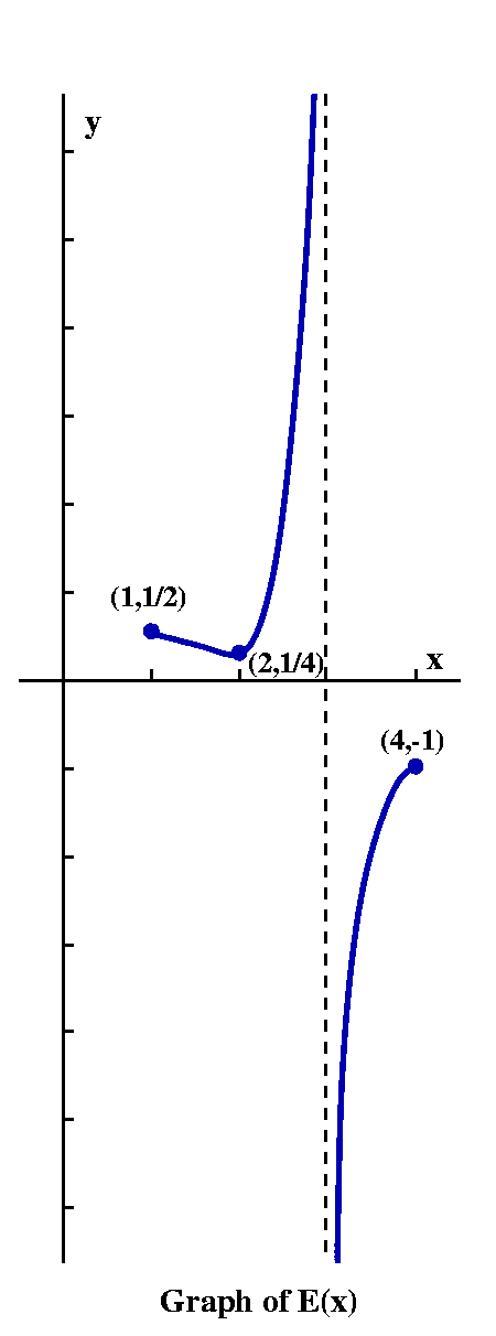 | |
|
What happens in the last chunk, for 3 to 4? Since K(4)=-1,
E(4)=1/-1=-1. Because K(x) is negative in 3<x<4, E(x) must be
negative also. But you've got to again think carefully and
critically. Let me make x move "left" from 4 in this case, move left
from 4 to 3. K(x) will then move from -1 towards 0, always being
negative. 1/K(x) will be negative, and its magnitude (size!) will be
the reverse of K(x)'s: K(x) small <==> E(x) large. So as x moves from
4 to 3, K(x) moves from -1 to 0 and E(x) "moves" from -1 to ... very
large negative. How large? Well, golly, as large as "you" want: E(x)
will have no lower bound, and will "tend towards" what some
folks call "minus infinity". Again, the graph of E(x) has the line x=3
as a vertical asymptote on the right and on the left of x=3.
Finally, we read off the domain and range of E(x). The domain was [1,3) and (3,4]. The range was [1/4,infinity) and (-infinity,-1]. Sketching E(x) was a difficult problem. | ||
|
Exercise F Consider F(x), as defined by F(x)=K(1/x). Here all of the precise information in the table of K(x) can be used to produce "precise information" (points on the graph of F(x)). The only secret is to realize that in order to get the desired inputs to the K(x) function, we need to input the reciprocal numbers to the F(x) function. x | F(x) ------------------------------------ 1/4 | F(1/4)=K((1/(1/4)))=K(4)=-1 1/3 | F(1/3)=K((1/(1/3)))=K(3)=0 1/2 | F(1/2)=K((1/(1/2)))=K(2)=4 1/1 | F(1/1)=K((1/(1/1)))=K(1)=2Yes, I know that 1/1 is just 1 but it seemed more natural to me to write it as 1/1. We can now graph these 4 dots and try to interpolate the remainder of the graph of F(x). The logic is parallel to but not identical with what we've just done. For example, as x "travels" from 1/4 to 1/3, 1/x goes from 4 to 3 (backwards?), and K(x)'s values go from -1 to 0, increasing. Each of the other intervals is similar. The domain of F(x) is [1/4,1/1]. The range is [-1,4], the same as the original range of K(x). So the "picture" is flipped, left to right, and then there is some strange proportioning going on: the stretching/compressing isn't the same in different intervals. | 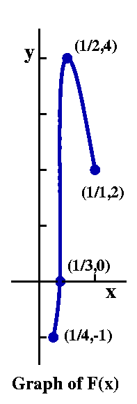 |
Fictions about rates of change
Mostly this course is about myths and, not lies, precisely, not
exaggerations, but certainly idealizations of reality, which
may not exist in any strict sense. I discuss this briefly before
we fling ourselves into the ideal swamp of calculus.
All of my warnings are correct. More or less, all of these rates are indeed fictitious. But everyone who works in those areas uses these rates as "truth" and the uses are almost always very convenient, and very useful, indeed. So the ideas turn out to be useful fictions about rates of change. I'm going to try to follow the text now and briefly postpone a direct approach to rates by looking at something that might appear to be simpler.
Functions on the edge
What can we say about the behavior of functions near where they are
not defined? This is a bit silly, as written, and I need to be much
more precise. But first let me give two examples, one geometric and one
algebraic, and then try for a general description.
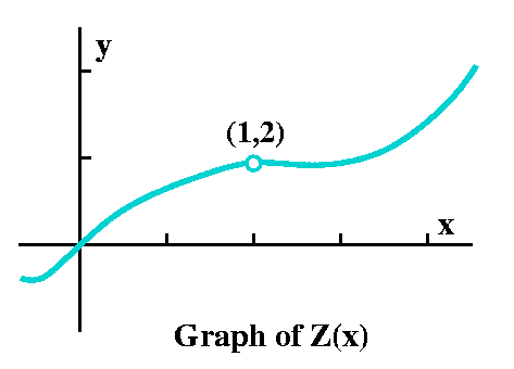 A geometric example
To the right is the graph of the function Z(x). I choose, by the way,
to specify only one point exactly on this coordinate plane, and that
point, (2,1), is supposed to be the one point which is a hole in the
graph!
So you are supposed to see, in this case, a function whose domain is all of the real numbers except for x=2. Aside from that the graph is not remarkable at all. My question for you to ponder is: what happens to the values of Z(x) as x moves towards 2? Again with the "kinetic" words: I am sorry, but that's how I think of it. O.k., rephrasing, if you think of Z(x) as a machine with an input and an output (no, not a biological model with an input and an output, too easy a joke!) then we could imagine putting in values of x close to 2 and inspecting the values of Z(x) which come out, and trying to see if there is any "simple" sense which can be made of them. Please, the picture and the question are probably (I hope!) almost too easy. I hope that you look at the picture and almost can declare that the values of Z(x) for x close to 2 (but not x=2!) are close to 1. That's the answer I want.
Important!
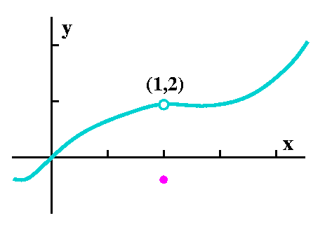
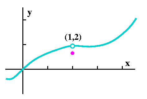
One thing I could use to confuse you: I could have given Z(x) a value
at x=2. Below that's the violet (magenta?) dot in the graphs. Then
(this is important!) any value I might choose to assign to Z(2) won't
change the answer to the question I originally asked, "What happens to
the values of Z(x) as x moves towards 2?" or to the thought
experiment, "Put in values of x close to 2 but not equal to 2
and inspect the results." So the answer would be the same if
the graph of Z(x) were any of the pictures below. I did not
emphasize this enough in class.
 Same answer |
 and same answer |
 and again, the same answer! |
An algebraic example
I defined the function Q(x) by the equation
Q(x)=[sqrt(x)-2]/[x-4]. Now and in the remainder of the course, when a
function is defined by an algebraic formula, the domain to be used is
"all the x's that allow everything to work". In this case, keeping in
mind the restrictions imposed by our manners
stated previously, we see that because of the square root, we can only
have x>=0. But also x-4 should not be 0. So the domain of Q(x)
should be [0,4) and (4,infinity). What happens to Q(x) when x gets
close to 4? We could try various approaches. One might be to
plug in numbers, not that there's anything wrong with that. I don't
especially want to compute values of Q(x) because that seems so
... "dirty". Wait. I have a silicon friend who has volunteered. My
friend gives me the following evidence:
  x     |    Q(x)
-------------------
  3     |  .26795
  3.5   |  .25834
  3.9   |  .25158
  3.99  |  .25016
  5     |  .23607
  4.5   |  .24265
  4.1   |  .24846
  4.01  |  .24984
The first 4 lines of the table give x's getting close to 4 from the left, and the next 4 lines five x's getting close to 4 from the right. Please look for the patterns, and see if the values of Q(x) seem to be getting close to "something".
We will use algebraic manipulations to be even more certain that the values are getting close to a unique "something", and to identify with precision what the "something" is. There are various tricks, almost all of which have been in use for hundreds of years. Here is one version that works with Q(x):
      [sqrt(x)-2]   [sqrt(x)+2]    [{sqrt(x)}2-22]        [x-4]             1
Q(x)= ----------- · ----------- = ---------------- = ---------------- = -----------
         [x-4]      [sqrt(x)+2]   [x-4][sqrt(x)+2]   [x-4][sqrt(x)+2]   [sqrt(x)+2]
Therefore, if x is not equal to 4, Q(x) can also be
described by the formula 1/[sqrt(x)+2]. I am trying to be almost
excruciatingly careful here. The reason I added the phrase "if x is
not equal to 4" is that in the algebra above we
canceled x-4 on the top and bottom. This step is only valid if the formula
canceled is not 0.
The advantage to having an alternative description of Q(x) is that maybe this one is not so sensitive to behavior near 4. Indeed, if we look at 1/[sqrt(x)+2], I hope it is not difficult for you to see that when x creeps (?) close to 4, this formula creeps close to 1/4. So Q(x) gets close to 1/4 when x gets close to 4, and changing the formula algebraically is one way to see this.
More from my silicon friend
O.k., my pal is electronic. But let us see what else it could tell
us. I asked for my friend's response to a request for Q(4.000000001)
(yeah, that's 4 plus a little bit, where the little bit is
1/1,000,000,000). If the algebra is correct, we'd hope that the
response is quite close to 1/4. The actual answer I got is 0. (Huh?)
On the other side, when Q(3.99999999) was requested, the answer was
.2, again not very close to 1/4. What is going on? The computations
are being done with about 10 decimal digits of accuracy. I'm asking
much to much of the program to give me accurate answers at the very
edge of its powers. You may need to keep this in mind when you use
electronic computational help.
|
The wonder of human vision There's another way to use computational data. Tabular data is nice, but the human brain, I have been told, has an enormous amount of its processing power devoted to analysis of images. We can ask that machine produce a picture of Q(x). One picture is shown to the right. The "machine" creates the picture by taking a bunch of data points and connecting the dots. The chance that one of the data points is a sample at exactly x=4 is small, so the machine isn't likely to run into much trouble. And human eyes like the picture, and the picture certainly seems to confirm that when x gets close to 4, Q(x) gets close to 1/4. | 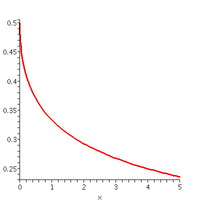 |
Limits
Well, I wrote three "excitement marks". The phenomena we have
been discussing are called limits. There are standard phrases to say,
and standard ways to write what we have been doing.
In the first example, we would say that, "The limit of Z(x) as x approaches 2 is 1." The notation used is limx-->2Z(x)=1. I like the little arrow underneath. In the second example, the notation is limx-->4Q(x)=1/4.
The whole limit idea is supposed to encapsulate the behavior of a function near, but not necessarily at the value. Here's where I recommend you begin reading chapter 2 of the text book.
Taxes, again?
I tried to revisit our two-bracket example of a tax
function. So:
      { (1/10)x if x<=10,000
T(x)= {
      { (2/10)x if x>10,000
What can you tell me about limx-->10,000T(x)? We discussed
this politely, as always (why does the guy in the front of the room
always talk so loud, though?). If x is near 10,000, and x is
above 10,000, then T(x) will be near 2,000. If x is near
10,000, and x is
below 10,000, then T(x) will be near 1,000. So there does
not seem to be one unique number that describes any sort of
clustering tendency for T(x) when x is near 10,000. Therefore, I will
say that limx-->10,000T(x) does not exist.
Yes, there are "one-sided" limits: look at the text, and I will mention them next time. But the genuine article, the two-sided limit, the one that's supposed to somehow, all by itself, represent T(x) for x near 10,000, does not exist. I remind you that this T(x) formula was one we had to fix, because it also did not adequately reflect certain societal requirements. Tricky, tricky!
QotD
Look at the quotient
1   1
- - -
x   2
-----
(x-2)
and use algebra to try to find the limit as x-->2 of this formula.
HOMEWORK
Please begin to read chapter 2. Please hand in these problems at
Thursday's recitation:
1.3: 12, 50, 61, 64
2.1: 1, 2, 5, 6
You will need to read 2.1 to understand the notation
in some statements of the problems.
Word of the day
Efficacy: capacity or power to produce a desired effect.
24 students indicated they were taking the course because it was "required". 32 wrote specific majors which needed calculus. Another 25 just remarked that Math 135 was needed by some unspecified major.
One brave student wrote that the course would "help me be successful", and another was taking the course "to get an A": I guess these were the optimists.
The idealists were few. A few students wrote such statements as, calculus is "kinda fun", "I enjoy math", and, better, "I love math".
So the overwhelming number of students are in Math 135 due to some outside compulsion: a lovely situation.
My job here is to teach math, and, I hope, to show you that the material is interesting and relevant. Let us see if I succeed. I certainly hope I will succeed.
I wrote Schedule X of the U.S. income tax form 1040 on the board as a function (look at the end of the last lecture). It is quite fascinating, and the details are complicated to me. By the way, I will mention Schedule X to any one who complains later in the course about the complexity of a computation! Understanding T(x), the Federal tax owed, as a function of the individual's taxable income takes some effort. I first wanted to assure myself that people understood how to compute T(x), so we discussed what the tax owed on an income of $35,000 would be: T(35000) would be computed using the third line of the table. It would be 4000 plus 25% (a quarter) of the amount over 29050, so 4000+(1/4)(35000-29050) which a calculator tells me is 4000+1487.5, or $5487.50. But as we consider the information defining T(x), there seem to be a bunch of almost random-looking numbers scattered. I mean, why is there 14,325.00? Why is there $35,717.00? The formulas for T(x) are all pieces of straight lines, which is why such a function is frequently called a piecewise-linear function.
Since I thought the intricacies of the real thing were perhaps too much for us, I decided to try to analyze a toy example.
Toy taxes
We could begin with a flat tax. Here the idea is that the tax
rate stays the same for everyone. For example, we could ask that
people owe 10% of their income: there are no tax brackets. Thus in
this scheme, T(x)=(1/10)x for all x>=0. Taxes don't just earn
revenue for government, of course. They are also frequently used as a
way of encouraging certain social policies. Therefore many localities
don't have a flat tax. The belief is that, somehow, if x is large,
then a higher proportion of x should be demanded as tax. Such a tax
system is frequently called progressive.
For example, we could complicate our original flat tax by asking that the tax rate be 10% for x's less than (or equal to!) 10,000, and the rate be 20% for incomes above 10,000. This seems imply that if we want to write a piecewise specification for this T(x), it might be
      { (1/10)x if x<=10,000
T(x)= {
      { (2/10)x if x>10,000
Is this a satisfactory formula? Well, what would the tax be for an
income of 9,999? I guess T(9999)=999.9. If income, x, increase by,
say, two bucks, what would the tax be using this scheme? T(10001),
would be (2/10)(10001)=2000.2. Let's see: earning two more dollars
increases the tax to be paid by over a thousand dollars! That doesn't
seem sane or fair (of course, tax policy need be neither sane nor
fair!). But here is a social rule that people like: if the income
changes a small amount, then probably the tax owed should only change
a small amount. The problem might be easier to see on a graph of this
T(x). I cheated a bit on this graph. The horizontal axis and vertical
axis don't have equal units. 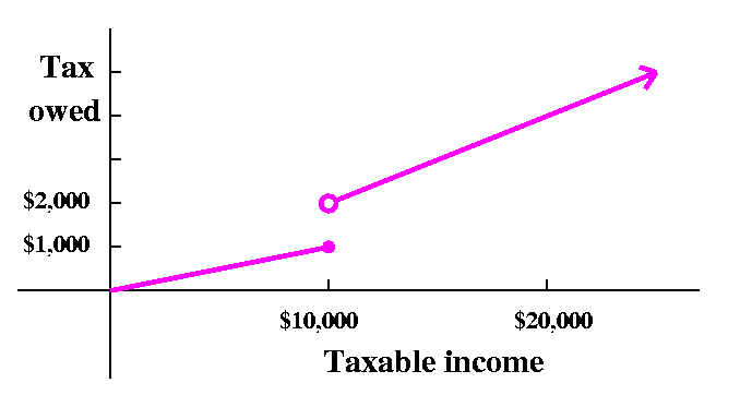
      { (1/10)x if x<=10,000
T(x)= {
      { (2/10)(x-10,000)+1000 if x>10,000
Now the graph looks nicer: there is no break, there is no jump in the
graph itself.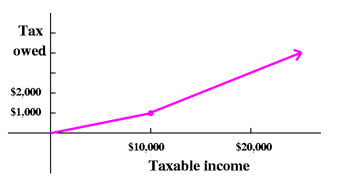
Before leaving the toy tax, I asked how to specify T(x) if we wanted a third rate, say 30% for incomes, x's, which are greater than 20,000. Again, some thought is required. When x is less than 20,000 and gets close to 20,000, then T(x) is given by (2/10)(x-10,000)+1000, so T(x) is getting close to (2/10)(20,000-10,000)+1,000, and this is 3,000. If we wanted to have three brackets, algebraically the formula would be
      { (1/10)x if x<=10,000
T(x)= { (2/10)(x-10,000)+1000 if x>10,000 and x<=20,000
      { (3/10)(x-20,000)+3000 if x>20,000
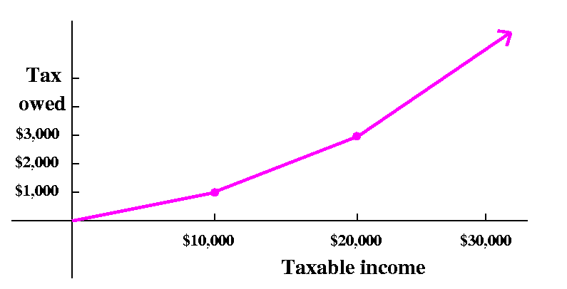
Well, back to Math 135. The due date for WeBWorK assignments for these sections (21, 22, and 23) will be Tuesdays at 9 PM. I'll have an office hour after class on Tuesdays on the Douglass campus. I should spend most of the 4th period in the Math Department's "satellite office", Chem 101. That's on the first floor of the building next to the Ruth Adams building. Please note that you don't need to do all of the WeBWorK problems in one session. The program will remember your progress. Also please try to keep up with the syllabus and suggested homework problems. You really won't be able to review them all immediately before an exam!

The trig functions
Sine and cosine are sort of the same, one is just shifted over a bit
compared to the other. The
tangent function is the quotient of sine over cosine. Wait: that's not
enough. Let's see:
Here is a graph of sine. From the graph the following can be seen:
I believe in radians as the true scale for inputs to the trig
functions. You should know the following coordinates of points on the
sine curve:
(0,0)
(Pi/6,1/2)
(Pi/4)
(Pi/3,sqrt(3)/2)
(Pi/2,1)
and from these you should be able to deduce lots of other values of
sine by symmetry and periodicity, since sine is periodic with period
2Pi:
sin(x+2Pi)=sin(x).
What are exact values of sin((7/4)Pi) and sin(-(5/2)Pi) and
sin((13/6)Pi)?
Pedagogical note After this course is over, I think forgetting
these exact values and freeing the few brain cells devoted to that
task should be an immediate goal. I believe that very few occasions
will require you to know the sine of Pi/6. But I am not in charge of
this course, and exams will demand exact answers to certain
questions. Sigh.
If you can demonstrate that you have 360 fingers and toes, I will attempt to get you an exemption to these requirements. Until then, please ... Also, as we will see later, doing calculus with degrees turns out to be much, much more awkward than doing calculus with radians.

Here is a graph of cosine. Please make sure that you know the
corresponding properties of cosine, such as:
There are many formulas from trig and precalc involving the sine and
cosine functions. I think we will generally reference only
I don't think you should forget every other formula but I doubt I will use others.
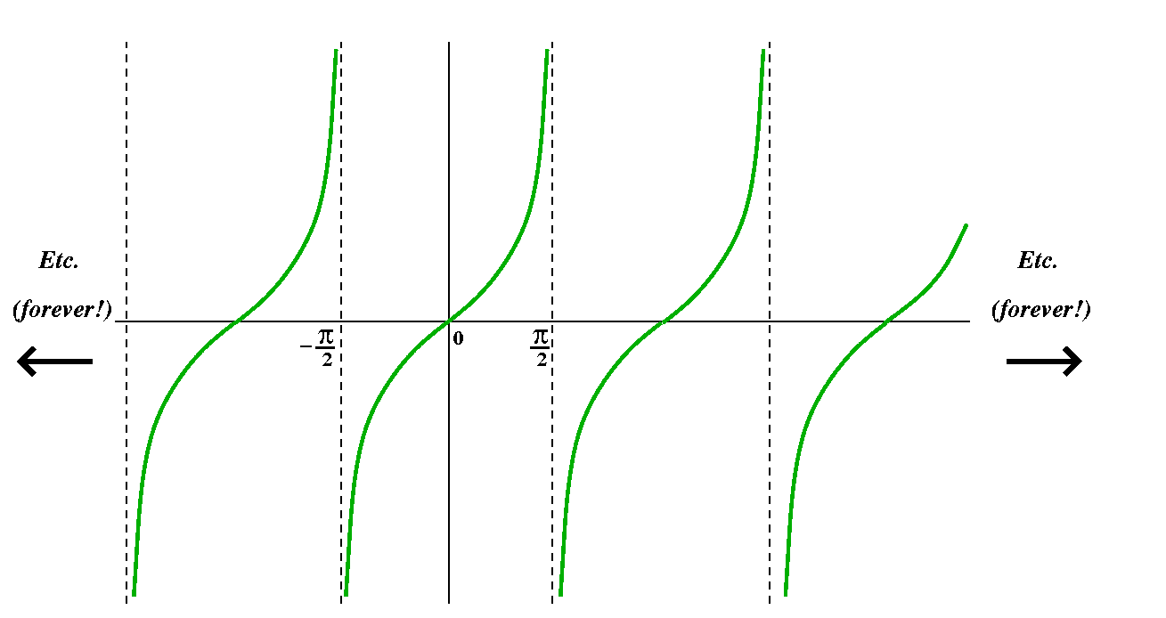
The tangent function is the quotient of sine divided by cosine. Since
cosine equals 0 when its input is an odd multiple of Pi/2, we should
expect weird behavior near odd multiples of Pi/2. The result is a
collection of vertical asymptotes. Etc., etc.
You are supposed to know all about these functions
already. Read the (expensive) text if you need more review,and do
the homework problems!
|
Exercise A Suppose A(x) is defined by the equation A(x)=-K(x). What does the graph of A(x) look like? What are its domain and range? This minus sign is on the outside of K(x), so it will primarily affect the range, the collection of outputs. In fact, we can use the table of K(x)'s values to write: x | A(x)=-K(x) --------------------- 1 | A(1)=-K(1)=-2 2 | A(2)=-K(2)=-4 3 | A(3)=-K(3)=0 4 | A(4)=-K(4)=-(-1)=1If you plot these points and try to interpolate a graph of the function A(x), you will see that it is the graph of K(x) "reflected" across the horizontal axis. The domain stays the same: 1<=x<=4, but the range changes to [-4,1]. It is conventional to write the more negative number on the left when using interval notation. |
 |
|
Exercise B Suppose B(x) is defined by the equation B(x)=K(-x). What does the graph of B(x) look like? What are its domain and range? This minus sign is on the inside of K, so it will primarily affect the domain, the collection of inputs. In fact, we can use the table of K(x)'s value's to write values of B(x). But here we need to be slightly tricky. To get values that are acceptable to B(x)=K(-x), we need to change the sign of the x's: x | B(x)=K(-x) -------------------------- -1 | B(-1)=K(-(-1))=2 -2 | B(-2)=K(-(-2))=4 -3 | B(-3)=K(-(-3))=0 -4 | A(-4)=K(-(-4))=-1The graph of B(x) turns out to be the graph of K(x) flipped over the vertical axis, the y-axis. The domain is [-4,-1] and the range is the same as the range of K(x), -1<=y<=4. |
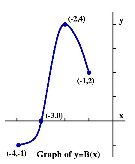 |
|
Exercise C Suppose C(x) is defined by the equation B(x)=3K(x). What does the graph of C(x) look like? What are its domain and range? The 3 is on the outside of K, so it will primarily affect the range, the collection of outputs. In fact, we can use the table of K(x)'s value's to write values of C(x). But here we need to be slightly tricky. To get values that are acceptable to C(x)=3K(x), we need to multiply K(x)'s values by 3: x | C(x)=3K(x) ---------------------------------- -1 | C(1)=3K(1)=3·2=6 -2 | C(2)=3K(2)=3·4=12 -3 | C(3)=3K(3)=3·=0=0 -4 | C(4)=3K(4)=3·-1=-1If we plot these points and interpolate correctly you should see that the graph of C(x) has domain [1,4] and range [-3,12]. The graph is K(x)'s graph stretched vertically by a factor of 3. |
 |
|
Exercise D Let's try D(x)=K(3x). Maybe this was the most difficult. The "3x" makes one think of stretching again, maybe in the domain. In fact, it is the opposite of stretching, a sort of compressing. For example, we know that K(1)=2. What can we deduce about D(x)=K(3x)? In order that 3x be equal to 1, we need to take x=1/3. Therefore D(1/3)=K(3·(1/3))=K(1)=2. Wow! So the 3x has the effect that to deduce values of D(x) from known values of K(x), we must divide the inputs to D(x) by 3. So here in tabular form, is our information about D(x): x | D(x)=K(3x) -------------------------------------- 1/3 | D(1)=K(3·1/3)=K(1)=2 2/3 | D(2)=K(3·2/3)=K(2)=4 3/3 | D(3)=K(3·3/3)=K(3)=0 4/3 | D(4)=K(3·4/3)=K(4)=-1We can deduce the domain: x's with 1/3<=x<=4/3. And the range is the range of K(x) because the change is inside. So the range is [-1,4]. |
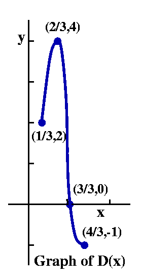 |
The QotD (Question of the Day) was to sketch the graphs of 1/K(x) and K(1/x). I think this is fairly difficult, so I asked that people work in groups of 2 to 4 individuals. As soon as I read the answers I will return here and discuss them.
HOMEWORK
Please read the sections of the book related to the first two
lectures, and at least look at the problems. Most of the exams will
resemble textbook problems. Also, spend a little time on WeBWorK.
 I began the class by writing some information about Quercus
imbrecaria, the Shingle Oak. To the right is a picture of one of
these. This is a species of tree, I have read, which is a "medium to
large oak reaching 50 to 60 feet" and it has "slow to medium growth of
12 to 18 inches per year".
Growth rate If the growth rate is 1 foot per year, that means
the tree will germinate from a seed and grow a foot in the first
year. (Maybe, but this a bit startling.) We can extrapolate a bit
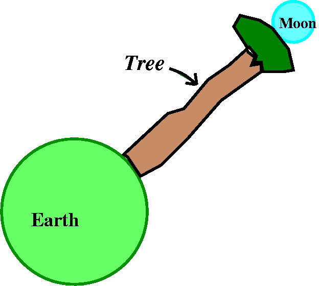
more. The distance from the Earth to the Moon is about 240,000 miles,
and if the tree grows 1 foot a year, then (since there are 5,280 feet
in a mile) the tree will hit the Moon in about a billion and a quarter
years. That's a tragedy. I show to the right a sort of impression of
what this might look like.
Well, of course just using the information "1 foot per year" as I did above is a bit simple-minded. The reality is that if H(t) is the height in feet of the tree after t years of growth, and if at germination we assert that H(0)=0, then initially growth is slow, and for large t's, the growth rate will be much less that 1 foot per year. "Growth rate" in the time interval between t1 and t2 (where t1<t2) will be the difference in the heights divided by the time span, or [H(t2)-H(t1)]/[t2-t1]. In reality the assertion that the growth rate is 1 foot per year means that for t1 and t2 somewhat away from 0 and not very large, this quotient will be approximately 1. Graphically, of course, the quotient [H(t2)-H(t1)]/[t2-t1] is the slope of the line connecting two points on the tree growth curve. It may be more than 1 (a good year, lots of moisture, sunlight, and required nourishment) or less than 1 (lousy weather, etc.).
What does a graph of the tree height look like? With the numbers 1 and
60 in mind, I suspect we may think that the collection of points whose
coordinates are (t,H(t)) may look as I display it.
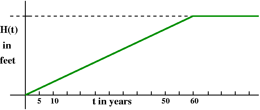 I actually doubt very much the graph is as simple as this: "piecewise
linear". I don't think that the tree grows until it gets to its
"ultimate height" and then just stays there. We will need more precise
language to analyze such questions.
I asked what the graph would look like. I got suggestions involving
"just any graph" (so maybe the tree height could be negative, or get
smaller as t gets larger?), or exponential (that would mean the tree
got really big really fast without any "ultimate" height. The
suggestion was made that the tree had logarithmic growth. Here we
needed to think a bit. I asked if log functions were bounded. For
example, consider log10. I know that
log10(1,000)=3, and I can even find a number W so that
log10(W)=7: take W=10,000,000 (seven zeros). I asked if we
could find a number V so that log10(V)>238. We thought
for a while. I finally suggested V=103,070. This will
work. So log10 is not bounded and couldn't be a
model of tree growth.
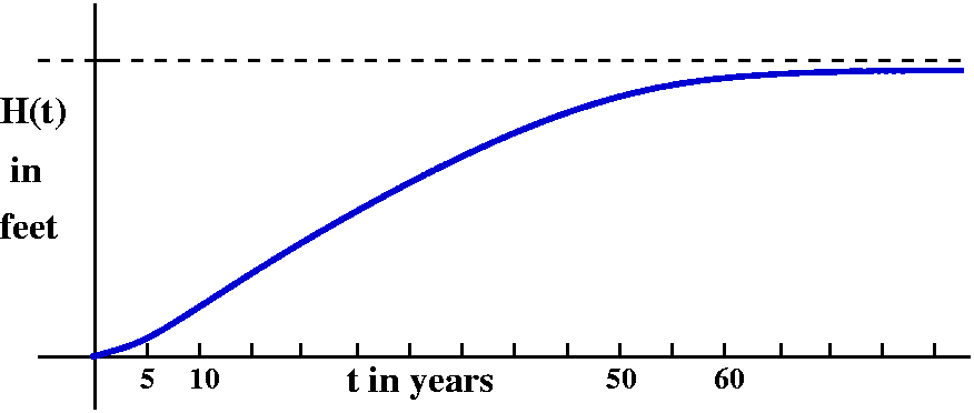 In fact, tree growth probably looks more like the graph displayed to
the right here. It is a complicated function, and even so, it is
really greatly simplified from reality, because I don't think that the
growth is ever as smooth as what is shown. Later in the course I will
try to return to this model, equipped with some vocabulary and
notation, and get a function that models the growth shown (the
logistic function).
The course is not a "pre-professional" course for math or CS or engineering majors. Those students should take Math 151. It is a course meant for students in certain biological sciences and intending to major in business areas. I will try to show the value of the vocabulary and techniques of calculus. This is my job, but I can succeed only with your good will and effort.
Grading I'll give two in-class exams (100 points each) and there will be a uniform (not written by me!) course final (200 points). Tentatively, I will make up a score of 150 points for the following activities: WeBWorK, textbook homework problems, quizzes in recitation, and activities in lecture.
Now, the world's quickest review of precalculus. (Look at sections 1.1 and 1.2 of the text.) This is supposed to be a review. If the material is not familiar, you must do many of the problems in the first few sections of the text.
Schedule X Single

If taxable income is
over-- 	        But not over-- 	The tax is:
$0 	        $7,150 	        10% of the amount over $0
$7,150 	        $29,050 	$715.00 plus 15% of the amount over 7,150
$29,050 	$70,350 	$4,000.00 plus 25% of the amount over 29,050
$70,350 	$146,750 	$14,325.00 plus 28% of the amount over 70,350
$146,750 	$319,100 	$35,717.00 plus 33% of the amount over 146,750
$319,100 	no limit 	$92,592.50 plus 35% of the amount over 319,100
I would like to try to analyze this function next time.
The Question of the Day was "Why are you taking this course?" I will report on the answers later.
HOMEWORK
Look at WeBWorK. Look at the text. Do the homework problems. On
Thursday, please hand in 1.1: 30, 42 and 1.2: 12, 40.
Maintained by greenfie@math.rutgers.edu and last modified 1/18/2005.