01:090:101:21, Experimental Math, the sixth meeting

Diary for 01:090:101:21, Experimental Math, fall 2008

The sixth meeting, 10/13/2008

I hoped that representatives of other question teams will report on their results, and indeed, I happily give thanks to Mr. Zimmerman of the Toad Team for explaning a solution to question #4, and to Mr. Weiner of the Horse Team for explaining a solution to question #5.

I will continue to consider recursively defined sequences, but with a rather different perspective. We will look at numerical approximations, not exact formulas, and end up with some analysis of a non-linear recursive sequence, that is, one where there are powers greater than 1.

Fibonacci, again

fibon:=proc(n) option remember; if n<=2 then 1 else fibon(n-1)+fibon(n-2) end if end proc;

The phrase option remember; may be new to you. This is an instruction which asks Maple to store old values which have been computed. For a recursively defined function, this can be a big saving of time and space. On my home PC, computing fibon(10000) with this definition took about a tenth of a second. But then the next Fibonacci number, fibon(10001), took less than .001 seconds because the old values were saved. When doing recursion, such economies can be significant. Without the option remember phrase, computing fibon(25) took about .2 seconds, computing fibon(30) took 3 seconds, and computing fibon(35) took about 32 seconds. Each increase of 5 seemed to multiply the time needed by 10! I didn't want to wait for fibon(100). I don't even want to think about fibon(10000) computed this way, because the glaciers would return several times while it was computed.

I recalled our previous results, which included the following: if we defined the growth constants and coefficients correctly, then we can get a formula for the Fibonacci numbers.

> gr1 :=(1+sqrt(5))/2; gr2 :=(1-sqrt(5))/2;
> A := sqrt(5)/5; B := -sqrt(5)/5;
> v := n -> A*gr1^n  + B*gr2^n

Then v(n) is the same as fibon(n). But I wanted to consider some numerical aspects of this formula. It turns out that Maple needs to be encouraged to evaluate things numerically. Its native method is to consider algebraic behavior. Look at these commands.

> tan(log(sin(2)));
                                tan(ln(sin(2)))
> tan(log(sin(2.)));
                                -0.09537061787
> tan(log(sin(evalf(2))));
                                -0.09537061787

So we can get numerical values by entering an argument with a decimal point (this is called a floating point number) or we can use the instruction evalf which tells Maple to convert the argument into a floating point number. Let me try this with the numbers we got for the Fibonacci sequence.

> f1 := evalf(gr1); f2 := evalf(gr2);
                       f1 := 1.618033988
                      f2 := -0.6180339880
> fA := evalf(A); fB := evalf(B);
                       fA := 0.4472135954
                      fB := -0.4472135954
> vf := n > fA*f1^n+fB*f2^n; 
                                   n        n
                   vf := n -> fA f1  + fB f2 
> vf(n);
                           n                               n
   0.4472135954 1.618033988  - 0.4472135954 (-0.6180339880) 

> vf(10)
                          54.99999973

There is good agreement between the real value of fibon(10), which is 55, and this value predicted by the formula. In fact, we can do better. The contribution to the formula from the f2 term is really small when n is large. This is because |f2|<1 and high powers of numbers with absolute values less than 1 get small very fast. Look:

> vfbig := n -> fA*f1^n; 
                                         n
                      vfbig := n -> fA f1 
> vfbig(10)
                          55.00363585

The simpler vfbig formula is quite close to 55 when n=10. This formula is simpler and easier to compute.

Then I tried to see the evidence of closeness by creating a graph. But powers grow quickly (at least powers of numbers larger than 1). So a way to tame the powers is to use logs. Since log(A^B)=Blog(A), the n's in the exponent become multipliers, and something like 37ⁿ will be n·log(37). When graphed as a function of n, this is a straight line. Let's see what happens. I will try to comment on each command. I won't bother to show the output until the final graph.

Command What's going on?

A:=seq([n,log(evalf(fibon(n)))],n=1..20);

This creates a collection of pairs of numbers. The second element of each pair is the log of the n^th Fibonacci number.

plot({A},style=point);
This plots the points (the curly brackets are needed to keep Maple happy). Think of this as "experimental data". This is part of what is shown in the accompanying graph.

B:=seq([n,log(vfbig(n))],n=1..20);

Here are numbers created with a formula. We want to "see" how closely they match the experimental data.

plot({B});

This generates a "curve" (really a straight line!) connecting the formula's points.

with(plots):

This command loads a package which has lots of elaborate plotting programs. In particular one of its commands will allow us to display two plots together on the same axes.

pA:=plot({A},color=blue,thickness=2,style=point); pB:=plot({B},color=green,thickness=2);

This creates two plots, and assigns them to the names pA and pB.

display({pA,pB});

The display command tries to show both of the pA and pB graphs together. The graph which was created with this sequence of commands is shown to the right.

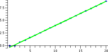This is pretty good agreement of a prediction by the formula. In this case, the "data" are the Fibonacci numbers, and the candidate for the predicting formula is vfbig.
In the graph to the right, the "true" values of the Fibonacci numbers are shown as blue points, and the green line which matches them fairly closely is the approximation gotten by taking the formula which only uses the bigger growth constant.
Remember that we used log(A^B)=Blog(A) so that the formula vfbig(n)=0.4472135954(1.618033988)ⁿ changed to log( 0.4472135954)+(1.618033988)n) which is -0.8047189564+(0.4812118246)n, a straight line. The slope is about 1/2: check with the picture, please.

Command	What's going on?
`A:=seq([n,log(evalf(fibon(n)))],n=1..20);`
	This creates a collection of pairs of numbers. The second element of each pair is the log of the n^th Fibonacci number.
`plot({A},style=point);`
	This plots the points (the curly brackets are needed to keep Maple happy). Think of this as "experimental data". This is part of what is shown in the accompanying graph.
`B:=seq([n,log(vfbig(n))],n=1..20);`
	Here are numbers created with a formula. We want to "see" how closely they match the experimental data.
`plot({B});`
	This generates a "curve" (really a straight line!) connecting the formula's points.
`with(plots):`
	This command loads a package which has lots of elaborate plotting programs. In particular one of its commands will allow us to display two plots together on the same axes.
`pA:=plot({A},color=blue,thickness=2,style=point); pB:=plot({B},color=green,thickness=2);`
	This creates two plots, and assigns them to the names pA and pB.
`display({pA,pB});`
	The display command tries to show both of the pA and pB graphs together. The graph which was created with this sequence of commands is shown to the right.
This is pretty good agreement of a prediction by the formula. In this case, the "data" are the Fibonacci numbers, and the candidate for the predicting formula is vfbig. In the graph to the right, the "true" values of the Fibonacci numbers are shown as blue points, and the green line which matches them fairly closely is the approximation gotten by taking the formula which only uses the bigger growth constant. Remember that we used log(A^B)=Blog(A) so that the formula vfbig(n)=0.4472135954(1.618033988)ⁿ changed to log( 0.4472135954)+(1.618033988)n) which is -0.8047189564+(0.4812118246)n, a straight line. The slope is about 1/2: check with the picture, please.

Something more strange ...
Now let's try something (maybe) more interesting.

> qfib:=proc(n) option remember; if n<=2 then 1 else qfib(n-1)+qfib(n-2)^2 end if end proc;

This recurrence is sort of the same as the Fibonacci rule, except that the "older" term, at n-2, is squared. I looked at this about 10 years ago, because I wanted to play and not work.

Here are a few terms. The option remember is very valuable in this case, because the terms get very big very fast. Look:

> seq(qfib(n),n=1..20);
1, 1, 2, 3, 7, 16, 65, 321, 4546, 107587, 20773703, 11595736272, 431558332068481, 134461531248108526465,
    186242594112190847520182173826, 18079903385772308300945867582153787570051,
    34686303861638264961101080464895364211215702792496667048327,
    326882906438860977154700726416259589991324369642278784888886456292858687899190928,
    1203139675581901612090570226442112857286846629264360460858253297925243660821490254528135651541164200107720542452689857, 106852\
    43452191713927725532729169455375269635012985468141090948568014383760138473439189515451932815803934664945833959351807102464428\
    8785133742254989047939450191041

These are really big numbers. For example, qfib(20) has 161 digits (a silicon friend assured me of this).

So we can take logs and graph. Here are some commands.

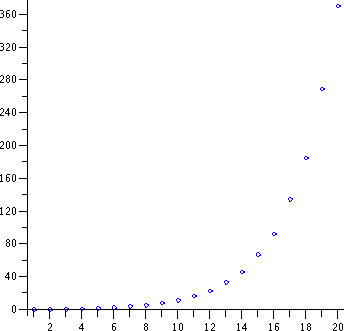
> QA:=seq([n,log(evalf(qfib(n)))],n=1..20):
> plot({QA},style=point,color=blue);

Taking logarithms of the qfib numbers makes them smaller, but not that much smaller. They still seem to grow, and not along a straight line! What could we do?

We could take another log, and see if that gets things under control, and if the resulting numbers seem more predictable. Here we go:

> Al2:=seq([n,log(log(evalf(qfib(n))))],n=1..30);
Al2 := [1, Float(-infinity)], [2, Float(-infinity)], [3, -0.3665129205], [4, 0.09404782792], [5, 0.6657298105], [6, 1.019781440],
    [7, 1.428967586], [8, 1.752921811], [9, 2.130847686], [10, 2.449802228], [11, 2.824303087], [12, 3.143026788], [13, 3.517451065],
    [14, 3.836174038], [15, 4.210598245], [16, 4.529321218], [17, 4.903745426], [18, 5.222468399], [19, 5.596892606], [20, 5.915615580],
    [21, 6.290039787], [22, 6.608762760], [23, 6.983186968], [24, 7.301909940], [25, 7.676334148], [26, 7.995057121], [27, 8.369481329],
    [28, 8.688204302], [29, 9.062628509], [30, 9.381351482]

The first two numbers are weird, because log of 0 is not defined. So I will restrict n, and make it at least 3 in all further computations. In particular, my seq command will have n=3..30.

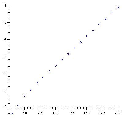
Now we can plot things, and so the result of the command plot({Al2},style=point,color=blue) is shown to the right.

What sorts of formulas would give us straight lines with log-log computation? Well, suppose you have A^{(B^C)}. Then log of this brings "down" the exponent, and we have B^C multiplied by log(A), that is, log(A)(B^C). Then log again. The result is log(log(A))+Clog(B). So if the resulting graph is a straight line, than C must be the variable, n, and A and B must be constants.

I would rather not lie to you. I didn't see things this clearly a decade ago. I think what I did was mess around with numbers. First, I looked at log(log(evalf(qfib(n)))). Here are some numbers:

> seq(log(log(evalf(qfib(n)))),n=3..20);
-0.3665129205, 0.09404782792, 0.6657298105, 1.019781440, 1.428967586, 1.752921811, 2.130847686, 2.449802228, 2.824303087, 3.143026788,
    3.517451065, 3.836174038, 4.210598245, 4.529321218, 4.903745426, 5.222468399, 5.596892606, 5.915615580

This didn't give me much insight. So I looked for how these numbers changed – that is, I wanted to understand the slope of the "line" that seemed to appear.

> seq(log(log(evalf(qfib(n))))-log(log(evalf(qfib(n-1)))),n=4..30);
0.4605607484, 0.5716819826, 0.3540516295, 0.409186146, 0.323954225, 0.377925875, 0.318954542, 0.374500859, 0.318723701, 0.374424277,
    0.318722973, 0.374424207, 0.318722973, 0.374424208, 0.318722973, 0.374424207, 0.318722974, 0.374424207, 0.318722973, 0.374424208,
    0.318722972, 0.374424208, 0.318722973, 0.374424208, 0.318722973, 0.374424207, 0.318722973

These are strange numbers. But they seem to be alternating, if you look at them a bit. They alternate (I'll look just at the last pair) between 0.374424207 and 0.318722973. What are these numbers? Well, it turns out there is a wonderful web page called the Inverse Symbolic Calculator which tries to identify numbers for you. The ISC can't identify these numbers, but their sum is 0.6931471 which the ISC guesses is an approximation for log(2) which you may know it as ln(2) and half of this by properties of logs is ln(sqrt(2)). This isn't what I actually did because I wasn't this clever. I just looked at the numbers, and then I guessed that the average "rate of change" or slope was log(2)/2 between integers because 0.6931471 looked familiar (the virtues of being a math nerd).

This means that log(log(evalf(qfib(n)))) should be approximately (1/2)*log(2)n. So let's look at what remains. Remember, if the original numbers are A^(Bⁿ) then what we are looking at is log(log(A))+log(B)n. If I want to see what else is there, I should take the log-log numbers and subtract{log(2)/2}n. I am assuming that log(B) is log(2)/2 which is log(sqrt(2)). Here are some commands which can be used to look at what's going on, and the resulting graph is shown to the right.

> points:=seq([n, log(log(evalf(qfib(n))))-(log(2.)/2)*n],n=2...30);
  [3, -1.406233692], [4, -1.292246533], [5, -1.067138142], 
  [6, -1.059660102], [7, -0.997047546], [8, -1.019666911], 
  [9, -0.988314626], [10, -1.015933675], [11, -0.988006407], 
  [12, -1.015856296], [13, -0.988005609], [14, -1.015856226], 
  [15, -0.988005610], [16, -1.015856227], [17, -0.988005609], 
  [18, -1.015856226], [19, -0.988005609], [20, -1.015856225], 
  [21, -0.988005608], [22, -1.015856225], [23, -0.988005607], 
  [24, -1.015856225], [25, -0.988005612], [26, -1.015856229], 
  [27, -0.988005611], [28, -1.015856228], [29, -0.988005611], 
  [30, -1.015856228]
> points := {%};
> plot(points, style = point, color = blue, symbolsize = 12);

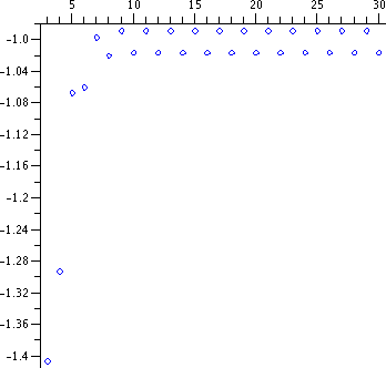The result of the plot command is shown to the right. I was very, very, very surprised to see this result. Actually, I wasn't clever enough to see things graphically when I started looking at this sequence. I first just had a mess of numbers to look at, and such a picture, exposing the weirdness and telling me what was true, was not something I thought of until weeks later!

What's happening?
In fact, qfib(2n) is approximately equal to A^{(sqrt(2)^2n-1)} where A is approximately 1.668751581493687... and qfib(2n+1) is approximately equal to B^{(sqrt(2)²ⁿ)} where B is approximately 1.693060557587684... and these formulas, for the odd and even subsequences, are different. This is a bit surprising. The earliest reference is here. I don't know an exact formula for the qfib's and I doubt there is one in terms of standard functions, but I am not sure if that is true (sorry!). This sequence is A000278 in Sloane's Encyclopedia.

Student "assignments"
I would be really happy if some students investigated some of the following questions.

What can you expect about a_n=a_n-1+(a_n-2)³? Discuss the behavior and get some numbers. The initial conditions are still 1 and 1.
What can you expect about a_n=a_n-1+(a_n-2)⁴? Discuss the behavior and get some numbers. The initial conditions are still 1 and 1.
What can you expect about a_n=a_n-1+(a_n-2)^power? Discuss the behavior and get some numbers. The initial conditions are still 1 and 1. What happens as the power indicated increases? The computations may not be so easy because the elements of the sequences get very large very fast.
What can you expect about a_n=a_n-1+(a_n-3)²? Discuss the behavior and get some numbers. Now the initial conditions could be 1 and 1 and 1. What happens?
What can you expect about a_n=a_n-1+(a_n-4)²? Discuss the behavior and get some numbers. Now the initial conditions could be 1 and 1 and 1 and another 1. What happens?
What can you expect about a_n=a_n-1+(a_{n-some integer})²? Discuss the behavior and get some numbers. Now the initial conditions could be all the 1's necessary. What happens?

Maintained by greenfie@math.rutgers.edu and last modified 10/12/2008.