Sequences and limits and algebra: sums of convergent sequences are convergent, and the limits are the sums of the limits. The saem with products, etc. I said that a more complete statement was in the textbook.
Sequences and limits and inequalities: if a_n<=b_n and a_n converges to L and b_n converges to M, then L<=M. We talked about whether just knowing that a_n converged implies that b_n would have to (it wouldn't).
A squeeze result: if a_n<=b_n<=c_n, and if a_n and c_n both converge with the SAME limits, then b_n would have to converge, and would share the common limit. I applied this to considering w_n=(3^n+4^n)^(1/n). This was difficult. Here I bounded w_n below by (4^n)^(1/n)=4 and above by (4^n+4^n)^(1/n)=2^(1/n)4 so the common limit was 4. This was not obvious. After much further discussion (including the asymptotic behavior of (3^n+4^n+5^n)^(1/n)!) we arrived at the following result: if A and B are positive, then the sequence (A^n+B^n)^(1/n) converges and its limit is the MAXIMUM of A and B (the largest of the two, or, if the two are equal, the common value).
I tried to echo the definition of infinite series which is in the book. I defined partial sums and sequence of partial sums and sum of an infinite series.
Problems due Tuesday: 9.3:16,17; 11.1:36,59,61; 11.2:10.
We discussed sequences and series again and did a homework problem. In this course we will have convergent and divergent improper integrals, convergent and divergent improper sequences, and convergent and divergent improper series: complicated terminology. I defined again what a sequence was, what a series was, and what the sequence of partial sums of a series was. This last concept allowed the definition of a convergent series and the sum of a convergent series (as the limit of the sequence of partial sums). We saw:
- If a series converges, then the sequence of individual terms must also converge, and the limit of this sequence is 0.
- The converse of the previous statement is in general false: that is, there are series whose nth term --> 0 but which do not converge.
For a while I would discuss series with nonnegative terms. For these series, the sequence of partial sums was increasing, and there were two mutually exclusive possibilities: EITHER the partial sums had some upper bound, and the series converged, OR the partial sums were unbounded.
Then I discussed the series sum (from 1 to infinity) of 1/(n^2) and sum (from 1 to infinity) of 1/sqrt(n). I remarked that so far we knew how to handle geometric series, and reminded people about such series. I asked if the series sum (from 1 to infinity) of 1/(n^2) was a geometric series. After some thought (What's a? What's r?) we seemed to convince ourselves that this series was not a geometric series.
Then I compared the partial sum 1+1/4+1/9+1/16 with an integral. By writing certain "boxes" correctly, we cleverly saw that this was less than 1 + the integral of 1/x^2 from 1 to 4. This integral I could compute, and we saw that the partial sum was less than 1+the integral from 1 to 4 of 1/x^2, and this was an overestimate which was easy to compute. Then I asked about the partial sum s_{700}, and we agreed that an overestimate was 1+the integral from 1 to 700 of 1/x^2: this was (if I remember correctly) 2-1/700. More generally we saw that just 2 alone was an overestimate of any partial sum of this series. Therefore the sequence of partial sums was bounded above, and the series converged.
The series sum_{n=1}^infinity 1/sqrt{n} was also not a geometric series. Here it turns out that the series diverged. For a partial sum one uses a comparison with the integral from 1 to T of 1/sqrt{x} dx, where T was some positive integer. This was 2sqrt{T}-2, and it --> infinity as T --> infinity. Since the partial sums are greater than this integral, the partial sums are unbounded.
I stated the Integral Test, as in the textbook. I then applied the Integral Test to analyze the convergence of sum_{n=1}^infinity 1/n, called the Harmonic Series. We saw that the series diverged since int_1^T=ln(T)-->infinity as T-->infinity. But I then asked: can we find a specific partial sum which is bigger than 100? I remarked that this is not a task to assign (directly!) to a computer for reasons which would become clear. I underestimated this partial sum by the integral from 1 to T+1 of 1/x, and therefore in order to be sure that the partial sum was > 100 I needed ln(T+1)>100, or T>e100-1. Since e^2 is approximately 9, it turns out that this means T should be about 1045 (the exponenet is halved). This is one heck of a lot of terms!
Further, we know that sum_{n=1}^infinity 1/n^2 converged. What partial sum will be within .01 of the true value? For this I split up the infinite series into s_N (a partial sum) + t_N, an "infinite tail", the sum from N+1 to infinity of 1/sqrt{n}. I overestimated this infinite tail by the integral from N to infinity of 1/x^2 which was 1/N. So s_{100} will be within the true value of the sum of the whole infinite series. In fact, Maple tells me that s_{100} is 1.634983903 while I just happen to know that the "true value" (to 10 decimal places) is 1.644934068. We are correct.
First I wrote a review of what we've done so far: for sequences with positive terms, bounded partial sums and covergence coincide, and unbounded partial sums and divergence coincide. Also, I rewrote the integral test, and remarked that it could be used to estimate infinite tails and also to get underestimates for partial sums. And I wrote that p-series (sum as n runs from 1 to infinity of 1/n^p) converges if p>1 and diverges otherwise.
I tried to give some reason for what we are doing now. That is, suppose one is trying to analyze some physical phenomenon, or maybe some computer algorithm. One gets experimental evidence and builds a mathematical model. Frequently the model involves some differential equation or maybe (especially in the case of the algorithm) what's called a difference equation. Then how to "solve" the equation? One can try for a polynomial solution, because polynomials can be easily computed (just multiplications and additions). But what happens? The "polynomial" solution turns out to have infinite degree -- to be a a power series. Then how can values of this solution be computed? The techniques which we are studying are used to give good approximations to these values, which are in turn used to go back and study the model, refining and changing it if necessary.
All this is too abstract. I then asked if sum_{n=1}^infinity 1/n^3 converged. I was told that it did (p-series, p=3>1). I asked what partial sum s_N=sum_{n=1}^N 1/n^3 was within .0001 of the "true value". I broke the series up into a partial sum, s_N, + an "infinite tail", t_N=sum_{n=N+1}^infinity 1/n^3 which I over estimated using the integral from N to infinity of 1/x^3. When I got that (1/2N^2) I asked what value of N would make this < .0001 and got one such N: 80 (I think). Maple reports that the partial sum here is 1.201979 while the "true value" is 1.20205: looks close, doesn't it?
I then asked the same questions for the series sum_{n=1}^infinity 1/(n^3+sqrt{n}). Here the question of convergence was settled with the following logic: since a bigger series converged, its partial sums are bounded, and therefore the partial sums of the smaller series must be bounded and THEREFORE (sigh!) the smaller series must converge. This comparison technique is used quite a lot. Again, the same partial sum will be within .0001 of the true sum.
I then asked the same questions of the series sum_{n=1}^infinity 1/(2^n + sqrt{n}). Here I said that each term satisfied the following inequality: 1/(2^n + sqrt{n})< 1/sqrt{n} and since 1/sqrt{n} diverged (p-series, p=1/2<1) can we assert that the smaller series must diverge? The answer is no, actually. So I asked how to determine that the series with general term 1/(2^n + sqrt{n}) converged? Well, look at the fastest growing part of the denominator (if that's what the bottom is called!): so compare this series with 1/2^n which is a convergent geometric series (a=1/2, and r=1/2 so |r|<1). Now how about a partial sum which is within .0001 of the true sum? Here the infinite tail of the overestimating series is sum_{N+1}^infinity 1/2^n, which is again a geometric series, with a=1/2^{N+!} and r=1/2. The sum is 1/2^N so to make this less than .0001 takes N=14 I think.
We then looked at a problem in the book for a while: for which p does the sum_{n=1}^infinity ln(n)/n^p converge? First we analyzed the case p=1. This can be done with the integral test, since ln(x)/x^2 has a neat antiderivative (look at the substitution ln(x)=u). It can also be done by comparison with the divergent harmonic series whose n'th term is 1/n since ln(n)>1 for n at least 3. Now ln(n)/n^p is also larger than ln(n)/n^1 for p<1, so, again, the series diverges for p less than or equal to 1. For p>1 the situation is more complicated. I suggested looking at an example. We considered the series whose nth term was ln(n)/n^1.0007. I rewrote this as 1/n^1.003 multiplied by ln(n)/n^.0004. This was motivated by the workshop problems involving rate of growth. Which of the functions (ln(x) and x^.0004) grows faster as x-->infinity? Here a graph of x^.0004 reveals very litte on the interval [1,5], say -- it essentially looks like a horizontal line at height 1. But l'Hospital's rule applied to the quotient ln(x)/x^.0004 actually shows that the limit is 0. Therefore the series with nth term ln(n)/n^1.0007 actually grows smaller than a series with nth term 1/n^1.0003, a p-series with p=1.0003>1, so it therefore converges. In fact, the series with nth term ln(n)/n^p converges if p>1.
I wrote the comparison test and the limit comparison tests, as in the text.
Problems due Tuesday: 11.3:22,23,34;11.4:32,36;11.5:28
I analyzed the alternating harmonic series, sum_{n=1}^infinity (-1)^{n+1}/n. We saw that the even partial sums moved "down" (decreased) and the odd partial sums moved "up" (increased). The even partial sums were bounded below by each of the odd partial sums, and the odd partial sums were bounded above by each of the even partial sums. Therefore the odd sums converged and so did the even sums (calling on results from sequences discussed a while ago). Since the difference between the odd and even partial sums were essentially the n^th term of the series and that -->0, we saw that the limits of the odd and even partial sums were identical and the series converged. I contrasted this result with the fact that the harmonic series itself (with all positive signs) did not converge.
I stated the Alternating Series Test as in the text. I gave another example of how this test applies. I also mentioned (and exemplified) that the nth partial sum of a series satisfying the hypotheses of the Alternating Series Test was within a_{n+1} of the true sum. So it is very easy to get an estimate of the error when using a partial sum in place of the full sum.
Then I copied the text's discussion of the fact that if sum |a_n| converges, then sum a_n must also converge. We discussed the text's discussion (!) and I tried to insure that people understood it. I gave a siumple example (something like the sum_{n=1}^infinity (cos(5n^3-33n^{3.6}+ etc)/n^5) of a complicated-looking series whose terms can be handled easily by realizing that values of cosine are between -1 and +1, so |(cos(5n^3-33n^{3.6}+ etc)/n^5)| is at most 1/n^5 and that series converges. Therefore by comparison, the original series with absolute value signs must converge, and by our result just verified, if the series with absolute value signs converged, then it must without absolute value signs. We noted that the converse to the result just used is generally false, and an example was the Alternating Harmonic Series.
I went on as in the text. I defined absolutely convergent series and conditionally convergent series. I translated our previous result as asserting that any absolutely convergent series must converge. I tried to give a metophor making sense almost surely only to me comparing series to folding and unfolding rulers with hinges. If the total length of the ruler totally unfolded is finite, then the lenght of the rule folded up any way must be finite.
The text then discusses the Ratio and Root Tests. I went on to discuss the first of these. First we reviewed again what a geometric series was. I asked how to identify a geometric series, and we discussed that for a while. Then I asked if the series sum_{n=1}^infinity (10^n)/n! converged. The first three terms seemed to be increasing. But what happens after, say, the 20^th term? The ratio between successive terms seems to always be LESS THAN 1/2. Then (this series has positive terms!) by comparison with a geoemtric series with ratio 1/2, this series converges. I then stated the Ratio Test carefully: if lim_{n-->infinity}|a_{n+1}/a_n| exists and equals L, then the series converges absolutely if L<1 and diverges if L>1. We applied the Ratio Test to the series sum_{n=1}^infinity (10^n)/n!, and had to be careful with the transition from compound fraction to simple fraction, and then with cancellation, using (n+1)!=(n+1)n!. Here we got L=0 so the series converged.
I then asked: For which x does sum_{n=0}^infinity ((-1)nx2n)/(2^2n(n!)2) converge? For those students who were still conscious (!) I explained that the sum of this series is important in analyzing the vibrations of a circular drumhead. We did this using the Ratio Test, and had to make sure that the algebra was correct. The answer: the series converges for all values of x.
I asked that students be sure to look at 11.5 and 11.6 before the workshop class tomorrow.
I began by discussing the Ratio and Root Tests. I tried to carefully apply these tests to Problem 5d) of the past workshop: sum_{n=1}^infinity {8/n^{1/5}}x^n. I used the Ratio Test as instructed, and got the results indicated in the answers: absolute convergence (and so convergence) if |x|<1, divergence if |x|>1. A separate investigation was needed for the other x's: for x=+1, p-series, p=1/5<1, divergence; alternating series test for for x=-1, convergence.
I introduced a heuristic idea for background on both the Ratio and Root Tests. Here's an appropriate definition for heuristic:
adj.
1. allowing or assisting to discover.
2. [Computing] proceeding to a solution by trial
and error.
If a_n is approximately arn, that is like a geometric series, then the quotient a_{n+1}/a+n is approximately like (arn+1)/(arn)=r, and the approximation should get better as n-->infinity. This gives a background for the Ratio Test. For the Root Test, if we assume that a_n is approximately arn and take nth roots, then some algebra shows that (a_n)1/n is approximately a1/nr, and we know
Limit fact 1 lim_{n-->infinity}a1/n=1 if a>0.
so we get the Root Test, similar to the Ratio Test but with (|a_n|)^(1/n) replacing |a_{n+1}/a_n|. I applied this to the example above, with a_n=8/n^{1/5}x^n. Here we needed to do some algebraic juggling and also needed
Limit fact 2 lim_{n-->infinity}n1/n=1.
We got results about convergence using the Root Test which were (comfortingly!) the same as what we got using the Ratio Test.
I analyzed the series sum_{n=1}^infinity n^n x^n, first with the Root Test and then with the Ratio Test. The Root Test was definitely easier, and the algebra gave n |x|, which (tricky!)-->infinity if x is NOT 0 when n-->infinity, but which has limit 0 when x=0. So the series converges ONLY when x=0. Then I tried the Ratio Test. Here some possibly tricky algebra is needed to get the same answer. Also needed is the following limit:
Limit fact 3 lim_{n-->infinity}(1+(1/n))1/n=e.
With this limit, the same result was gotten as with the Root Test, although with quite a bit more work. I then verified the limit, by taking ln of (1+(1/n))1/n and using l'Hospital's rule.
In general we have been studying Power Series. I defined a power series centered at c" it is sum_{n=0}^infinity a_n (x-c)^n, a sort of infinite analog of a polynomial. Almost all of our examples would have c=0.
Guiding questions:
- For which x does such a series converge? (Remark: such series always converge for x=0. Is there anything useful and general one can say about the x's for which the series converge?)
- What are the properties of the sum of such a series? (Still to be understood!)
- Why should we look at this? What are the rewards, and what are the reasons?
We concluded that if the series converged for |x|=R then it must
converge for x's with |x|
We saw even more from the comparison with geometric series. If we
wanted to analyze how to compute the series for |x|=r with r
The sum of a power series inside its interval of convergence
must be a continuous function.
This will be a partial answer to question #2 above, but much more and
much nicer things are actually true and will be discussed later.
Students should prepare to hand in these problems next Tuesday:
11.6:25,32;11.7:13,35;11.8:13,30.
I finished the theory of power series (as much as I would do):
Suppose now that a player wins $10 if the spinner hits red, loses $18
if it hits green, and wins $24 if it hits blue. What is the average
winning? It is (1/2)(10)-(1/3)(18)+(1/6)(24)=3. So a fair "entry fee"
to play this game would be $3: that is, in the long run, neither the
contestant nor the proprietor of the game would win/lose money if such
an entry fee were charged.
Now a more complicated game: consider a "fair coin" with a head and a
tail. Toss the coin until it lands heads up. How many different ways
are there for the game to play? It could land H (heads), 1/2 the
time. It could land tails then heads, TH, 1/4 of the time. It could
land TTH, 1/8 of the time. Generally, it could have the sequence
TTT(n-1 times)TTTH, which is n tosses, 1/(2^n) of the time. There are
infinitely many different ways for this game to end.
Suppose the proprietor of the game will pay the contestant n^2 dollars
if the game ends after n tosses. What is the average amount that could
be won in the game? Analogous to what was done above in the simpler
game with a finite number (just 3) outcomes, here the average winning
amount would be sum_{n=1}^infinity (n^2)/(2^n)?
Does this sum converge? That is, can one expect on average to win a
certain finite amount in this game? We used the ratio test to show
that it did indeed converge. But what is the sum, exactly?
Here we need to think a bit. The sum of the series sum_{n=1}^infinity
x^n is x/(1-x), the sum of a geometric series. The derivative of both
sides gives the series sum_{n=1}^infinity nx^{n-1} on the series side,
and on the other side (using the quotient rule) 1/(1-x)^2. If we
multiply both sides by x, we'll get sum_{n=1}^infinity nx^n on the
series side and x/(1-x)^2 on the function side. So if we let x=1/2,
the series will be sum_{n=1}^infinity n/2^n and the function value
will be (1/2)/(1-1/2)^2=2. So the sum of this series is 2.
To get n^2 to appear on top we need to differentiate again. That is,
take sum_{n=1}^infinity nx^n =x/(1-x)^2 and differentiate. The series
side becomes sum_{n=1}^infinity n^2 x^{n-1} and the function side
(again using the quotient rule) is (1+x)/(1-x)^3. If we multiply by x,
the series becomes sum_{n=1}^infinity n^2 x^n and the function side
becomes (x+x^2)/(1-x)^3. If we substitute x=1/2, the series side is
sum_{n=1}^infinity n^2/2^n (finally what we want!) and the function
side is (1/2+(1/2)^2)/(1-(1/2))^3 which is 6. So $6 is a "fair entry
fee" to pay the proprietor of this game. I don't think the sum is at
all obvious. What I've done is find what is called the
expectation of this game.
I announced that the next exam would be on the Thusday after
Thanksgiving, which is Thursday, November 29. It will cover
differential equations and the material of chapter 11. An old exam
will be gone over in the workshop session on Tuesday, November 27. A
draft of a formula sheet will be given out earlier.
We returned to power series, and used the general name, Taylor series,
to indicate that if f is the sum of a series, sum_{n=0}^infinity a_n
(x-c)^n, then a_n=f^{(n)}(c)/n!. The partial sum sum_{n=0}^N a_n
(x-c)^n is called the N^{th} Taylor polynomial. The difference between
the partial sum and the true value of the function is called the
remainder, R_N(x) (this is what I previously called the "infinite
tail", and is sum_{n=N+1}^infinity a_n (x-c)^n).
The game is to usefully estimate R_N(x) and use the idea that when the
series converges (R_N(x)-->0) then the series can be manipulated (inside
its radius of convergence) to yield other series which converge. The
manipulations can either be algebraic (add, multiply, etc.) or from
calculus (differentiate, integrate). So how to estimate R_N(x)? The
techniques we've already learned to estimate "infinite tails" can all
be applied here, but they can be supplemented by a powerful new idea.
Taylor's Theorem: f and T_N and R_N as before. Then |R_N(x)| is less
than or equal to (M_{N+1} |x-c|^{N+1}}/(N+1)!. Here M_{N+1} is an
overestimate of the absolute value of the (N+1)^{st} derivative of f
on the interval whose endpoints are c and x.
I indicated that I would try to show a lot of simple examples
explaining why Taylor's Theorem is useful both as a computational
mechanism and as a theoretical tool.
First looked at exp(x)=e^x. Here c=0 (almost always c=0,
actually!). Then all the derivatives of exp are exp, and
f^{(n)}(0)=exp(0)=1, so the Taylor series is
\sum_{n=0}^infinity(1/n!)x^n, a very very simple series. I applied the
Ratio Test to show that the radius of convergence was infinity
(because the limit was always 0, and didn't depend on x, and 0 is less
than 1). But how can one use the series to compute values of exp?
How can exp(-.3) be computed with an accuracy of .001? So we can try
to write exp(-.3)=T_N(-.3)+R_N(-.3), and select N (if we can) with
|R_N(-.3)| less than or equal to .001. If we can do that, then
T_N(-.3) is a finite sum and can be directly computed. So here R_N is
what? . Here M_{N+1} is an
overestimate of the absolute value of the (N+1)^{st} derivative of f
on the interval whose endpoints are c and x.
I indicated that I would try to show a lot of simple examples
explaining why Taylor's Theorem is useful both as a computational
mechanism and as a theoretical tool.
First looked at exp(x)=e^x. Here c=0 (almost always c=0,
actually!). Then all the derivatives of exp are exp, and
f^{(n)}(0)=exp(0)=1, so the Taylor series is
\sum_{n=0}^infinity(1/n!)x^n, a very very simple series. I applied the
Ratio Test to show that the radius of convergence was infinity
(because the limit was always 0, and didn't depend on x, and 0 is less
than 1). But how can one use the series to compute values of exp?
How can exp(-.3) be computed with an accuracy of .001? So we can try
to write exp(-.3)=T_N(-.3)+R_N(-.3), and select N (if we can) with
|R_N(-.3)| less than or equal to .001. If we can do that, then
T_N(-.3) is a finite sum and can be directly computed. So here R_N is
what? (M_{N+1} |x-c|^{N+1}}/(N+1)!. Here c=0 and x=-.3 and what
should M be? M is a max of the (N+1)^{st} derivative of exp (just exp)
on [-.3,0]. But exp is increasing so a max is just exp(0), which is 1,
There's NO N in the answer. This simplifies things a great deal. So
what we need is an N so that |-.3|^{N+1}/(N+1)!<.001 and think about
this: the TOP-->0 and the BOTTOM-->infinity, so we should expect some
N for which this is actually <.001, so I wrote a list of N!'s, which
seemed to grow very quickly. We found out that N=6 actually works, and
so T_6(-.3) will be within .001 of exp(-.3).
Then I worked on exp(2). Here the situation was more complicated. x=2
and c=0 and what is M_{N+1}? It is an overestimate of exp on
[0,2]. This is e^2. But we want to compute e^2? Isn't it silly to need
to know e^2 in order to compute e^2? Ahhhh ... but the key here is
OVERESTIMATE: loose information about e^2 can be converted to better
and better estimates. For example, e^2 is certainly less than 10
(since e<3, e^2<3^2=9<10). So we know that |R_N(2)| can be
overestimated by 10(2^{N+1})/(N+1)!. Now both the top (2^{N+1}) and
bottom ({N+1}!) go to infinity. The key here is that factorials grow
much faster than "geometric" growth. We saw this explicitly because I
wrote a list of powers of 2 and factorials for N going from 1 to
10. In this case we needed to go to N=8 to get T_8(2) within .01 of
the true value of e^2.
Note that life is actually a bit complicated here. One gets, even for
a fairly simple function (and exp is very simple in this context!)
that the N's can be different for different x's, and for different
error tolerances.
Then I tried to compute sin(2). For this I found the Taylor series of
sine. This involved taking derivatives of sine, and finding that these
derivatives repeated every fourth time (sine --> cosine --> -sine -->
-cosine --> sine). So the values at 0 (necessary for getting the
Taylor series) were 0, 1, 0, -1, etc. I wrote the Taylor series for
sine centered at 0: sum_{n=0}^infinity (-1)^n x^{2n+1}/{2n+1}!. To
compute sin(2), I needed again to estimate
(M_{N+1}|x-c|^{N+1}}/(N+1)!. Here how should we estimate M? We need to
know a useful max of the absolute value of some derivative of
sine. But, all of these functions (there are exactly 4 of them!) can
be estimated by 1 (amazing, and easy!). So if x=2 and c=0 we need
2^N/(N+!)! < .01. This can be done with, I think, N=7. We then
discussed what T_7(2) for sine. It is actually the first 4 terms of
the series: sum_{n=0}^4 (-1)^n 2^{2n+1}/{2n+1}!, since these terms go
up to DEGREE 7. This is a case where the number of terms and the
degree of the terms do NOT coincide.
I also mentioned the series for cosine: : sum_{n=0}^infinity (-1)^n
x^{2n}/{2n}!
I gave out a draft review sheet for the second exam, and a schedule
for the last part of the course.
I reviewed Taylor's series, the Taylor polynomial, and Taylor's
Theorem, with attention to the remainder estimate. The simplest
functions to apply this "machine" to are exp and sine and cosine
because these have simple families of derivatives. I reviewed much of
what we did last time, giving numerical evidence for the truth of our
estimate. For example, in the first problem we did then, the Taylor
polynomial T_6(-.3) is approximately .7408182625 while the "true
value" of exp(-.3) was reported by Maple to be .74089182207. This is
quite a bit more accurate than the pessimistic .001 error given by
Taylor's Theorem.
I remarked that the graph of sin x and T_7(x) (which is
x-(1/6)x^3+(1/120)x^5-(1/5040)x^7) when looked at on the interval
[0,2] were actually very close, certainly within .01, and that
therefore for many practical purposes the functions could be exchanged
with one another.
One application of such ideas could be to the evaluation of difficult
integrals. The example I chose to look at was the integral from 0 to
.3 of cos(x^2). This function actually arises in a number of
applications, such as optics. How could we compute int_0^.3 cos(x^2)dx
to an accuracy of .001? One technique might be to try to find an
antiderivative of cos(x^2). This turns out to be impossible (that is,
finding an antiderivative in terms of known functions). It isn't easy
to see that getting such an antiderivative is impossible. Another
method might be to use some numerical techniques to approximate the
integral, such as the Trapezoid Rule or Simpson's Rule. But there is
also a third approach, which I carried out in the lecture.
The Taylor series of cos(x) is sum_{n=0}^infinity (-1)^n/(2n)!
x^{2n}. I also know that the Remainder is going to be something like
M|x|^{a power}/{that power}! and that the M here will be at most 1,
because the derivatives of cosine are +/- sine and +/- cosine, and
these are all bounded in absolute value by 1. In fact, I know that the
Remainder will -->0 because factorial growth in the bottom will
overcome power growth in the top. So the series will actually equal
cosine for all x's. Then cos(x^2) is gotten by substituting x^2 in the
series for cosine, so we get sum_{n=0}^infinity (-1)^n/(2n)!
(x^2)^{2n} which is sum_{n=0}^infinity (-1)^n/(2n)! x^{4n} because
repeated exponentials multiply. If we want the integral of cos(x^2),
we just need to antidifferentiate the series sum_{n=0}^infinity
(-1)^n/(2n)! x^{4n}, treating it like an infinite polynomial. So the
result will be sum_{n=0}^infinity (-1)^n/(2n)! (1/(4n+1))x^{4n+1}.
This is then an indefinite integral, and we need to evaluate it at .3
and subtract off its value at 0. The value at 0 is 0, since all the
terms have powers of x in them. The value at .3 is sum_{n=0}^infinity
(-1)^n/(2n)! (1/(4n+1))(.3)^{4n+1}. This is actually an alternating
series, and its value can be approximated by a partial sum with
accuracy at least that of the first omitted term. But the third term
(with n=2) is actually less than .00001, so the integral is just the
sum of two fractions, the one with n=0 and with n=1. I did this
computation both in summation notation and by writing out the first
few terms, in order to give people practice in understanding "sigmas".
Then I went through problem 6 of the previous workshop, making sure
that the power series for arctan was discussed. I went through all
parts of the problem (a & b & c & d & e & f). The total number of
students present was the same as the number of parts in the problem.
I found a power series expansion for ln(1+x) by taking the derivative,
1/(1+x), setting it equal to a sum of a geometric series,
sum_{n=1}^infinity (-1)^n x^n, and integrating each term to get
sum_{n=1}^infinity (-1)^n/(n+1) x^(n+1). The radius of convergence of
the series resulting is 1, since the original geometric series
converges for |x|<1 and integration (and differentiation) don't change
the radius of convergence. I mentioned that ln(x) can't have a nice
Taylor series because it has a vertical asymptote at x=0, so
alternatively a Maclaurin series for ln x centered at x=1 is given by
rewriting the series just obtained: ln x= sum_{n=1}^infinity
(-1)^n/(n+1) (x-1)^(n+1).
I attempted to use the series just derived to show how ln(1.5) could
be computed to accuracy .00001 (1/100,000). Here I used the fact that
sum_{n=1}^infinity (-1)^n/(n+1) (.5)^(n+1) was an alternating
series. We found that n=10 would make (.5)^(n+1) certainly less than
1/(100,000) so that the partial sum of the first 19 terms would be
close enough. Here we needed results on alternating series and their
partial sums.
I remarked that the series for exp and sin and cos were widely used
for computation but the series for arctan and ln were not, becuase
they converged relatively slowly. The first three series converged
rapidly because factorials grow very fast.
Then I asked what x^{1/3} "looked like". This was very fuzzily
stated. To compute x^{1/3} one can use various buttons on a
calculator. For example, 8^{1/3} is 2. The computation is probably
done using some variant of Newton's method. That is, a starting
"guess" x_0 is gotten, and then x_{n+1} is some interesting (?)
rational combination of x_n, a recursively defined sequence. This will
tell you rather rapidly what x^{1/3} is like. But in some sense it
doesn't give you a feeling for the function. It is an algorithm, but
not with much information directly. For example, we know that if x is
close to 8 then x^{1/3} should be close to 2 (this is because x^{1/3}
is continuous). Maybe not even that is totally clear from the Newton's
method iteration.
I asked what the first Taylor polynomial of x^{1/3} centered at x=8
was. We found out that it was T_1(x)=2+(1/12)(x-8) (this is
f(8)+f'(8)(x-8) when f(x)=x^{1/3}). I asked people to graph T_1 and f
in the window 6
I chose this example so that the numbers would work up relatively
nicely when done by hand, but the general philosophy works with little
change in much more complicated situations. So one can frequently
"locally" replace a function by a polynomial.
I asked for questions about the material of chapter 11.
I did two problems from the text: #37 and #41 of section 11.10.
Then I began parametric curves. I first studied the "unit circle"
(x=cos t, y=sin t) and discussed how this compared with
x^2+y^2=1. There is more "dynamic" information in the parametric curve
description, but there is also more difficulty: two equations rather
than one.
I sketched (x=cos t,y=cos t) and (x=t^2,y=t^2) and (x=t^3,y=t^3): all
these are pieces of the line y=x: I tried to describe the additional
dynamic information in the parametric definitions.
I showed some parametric curves from book Normal Accidents by
Charles Perrow: pictures of ship collision tracks.
Then I tried to sketch the parametric curves (x=2 cos t, y = 3 sin t)
and (x=1+sin t, y= cos t -3) which I got from another textbook. The
first turned out to be an ellipse whose equation is (x/2)^2+(y/3)^2=1
and the second turned out to be a circle of radius 1 centered at
(1,-3). These curves intersect, but do they actually describe the
motion of particles which have collisions? Well, one intersection is a
collision and the other is not (this is generally not too easy to
see!).
I tried to describe the parametric curves for a cycloid. This is done
with a slightly different explanation in section 10.1 of the
text. This took a while.
Then I described my "favorite" parametric curve:
(x=1/(1+t^2),y=t^3-t).
Next time: calculus and parametric curves. These problems are due
Tuesday: 10.1: 12,18; 11.11: 11,14; 11.12: 5,28.
I started again to discuss parametric curves, beginning by sketching
again my favorite, x=t^3-t, y=1/(1+t^2). I wanted to do calculus with
parametric curves. The object was to get formulas for the slope of the
tangent line to a parametric curve and for the length of a parametric
curve.
If x=f(t) and y=g(t), then f(t+delta t) is approximately
f(t)+f'(t)delta t +M (delta t)^2 (this is from Taylor's Theorem). Also
g(t+delta t) is approximately g(t)+g'(t)delta t +M (delta
t)^2. The reason for the different "M" is that these are different
functions to which Taylor's Theorem is being applied. Then we analyze
the slope of the secant line, (delta y)/(delta x): this is
(g(t)+g'(t)delta t +M -g(t))/(f(t)+f'(t)delta t +M (delta t)^2)
and we see that the limit as delta t --> 0 must be g'(t)/f'(t), and this
must be the slope of the tangent line, dy/dx. The formula in the book,
developed in a different way using the Chain Rule, is also nicely
stated in classical Leibniz notation as (dy/dt)/(dx/dt).
I applied this to find the equation of a line tangent to my favorite
curve, x=t^3-t, y=1/(1+t^2), when t=2. I found a point on the curve
and I found the slope of the tangent line, and then found the line. It
sloped slightly down, just as the picture suggested. Then I found the
angle between the parts of the curve at the "self-intersection",
t=+/-1. This involved some work with geometry and with finding the
slopes of the appropriate tangent lines. The best we could do is with
some numerical approximations to the angles.
I asked people what the curve x=sin t+2 cos t, y-2 cos t - sin t,
looked like. We decided it was bounded because sine and cosine are
always between -1 and +1, so the points of the curve must be in the
box -3
I remarked that for "well=behaved" parametric curves, vertical
tangents occur when dx/dt=0, and horizontal tangents, when dy/dt=0.
Then I briefly discussed the arc length between (f(t),g(t)) and
(f(t+delta t),g(t+delta t)). With the approximations f(t+delta
t)=f(t)+f'(t)(delta t) and g(t+delta t)=g(t)+g'(t)(delta t) we saw
that this distance (using the standard distance formula) was
approximately sqrt(f'(t)^2+g'(t)^2) delta t. We can "add these up" and
take a limit. The length of a parametric curve from t=START to t=END
is the integral_START^END sqrt(f'(t)^2+g'(t)^2) dt.
How useful is this formula? Maybe not too. As a first example, I tried
to find the length of the loop in my favorite parametric curve. I
ended up with int_{-1}^{1} sqrt((3t^2-1)^2+(-2t/(1+t^2)^2)) dt, which
is a very intractible integral. I would not expect to be able to use
the Fundamental Theorem of Calculus to "do" this integral. That is, I
would not expect that I could find an antiderivative in terms of
familiar functions. I'd expect to need to compute this integral
numerically, approximately.
The integrand in the arc length formula for parametric curves is
horrible if one wants to compute the length exactly. It is difficult
to find many examples. Here are a few, and section 10.3 has others. I
first looked at x=cos t and y=sin t. for t=0 to 2Pi. This is, of
course, the unit circle. I found the length of this curve and it was
easy because the integrand turned out to be exactly 1!
I looked at the curve x=(1-t^2)/(1+t^2) and y=2t/(1+t^2) for t=0 to
t=1. This looks initially very forbidding. But direct computation of
sqrt(f'(t)^2+g'(t)^2) yields (miraculously?) 2/(1+t^2). This
integrated from 0 to 1 is exactly Pi/2. Remarkable! (In fact, 10.3's
problem section has a number of such "accidents" which take a great
deal of dexterity to create!) What "is" this curve? It is a curve
going from (1,0) (when t=0) to (0,1) (when t=1) and has length
Pi/2. Sigh. It is one-quarter of the unit circle! This is a famous
"rational parameterization" of the unit circle: a description using
rational functions, quotients of polynomials.
These problems are due Tuesday: 10.1: 9,10; 10.2: 3,8; 10>3: 4,7.
We talked a bit about parametric curves, and then began polar
coordinates. I "wrote" an excerpt from a really lousy adventure novel.
I introduced polar coordinates and got the equations relating (x,y) to
(r,theta). I looked at the point (3,0) (in rectangular coordinates)
and saw that there were infinitely many pairs of polar
coordinates which described the position of this point (I gave
examples). I remarked that in many applications and computer programs,
there were restrictions on r (usually r is non-negative) or on theta
(say, theta must be in the interval [0,2Pi) or in the interval
(-Pi,Pi] or something) in an effort to restore uniqueness to the polar
coordinate representations of a point's location. No such restrictions
were suggested by the text used in this course. I sketched the regions
in the plane specified by the inequalities 2
What about other polar curves? We spent some time sketching the curve
r=2+cos theta. This curve was inside the circle r=3 and outside the
circle r=1. I tried to sketch what it might looklike. Even with this
rather simple curve we got into difficulties. It looked "smooth" but
when theta was 0 or Pi, it wasn't clear whether the curve has a
"point", that is, a cusp.
Therefore I studied tangent lines to polar curves and we derived a
formula in rectangular coordinates for the slope of a tangent line to
a polar curve r=f(theta). Here I noted that polar curves were a
special type of parametric curve. So, since x=r cos theta, we know
that x=f(theta)cos theta and y=f(theta)sin theta. Then using the ideas
previously derived, namely that dy/dx= (dy/d theta)/(dx/d theta), I
got the formula in the book for dy/dx in polar coordinates.
I used this to find the equation of a line tangent to y=2+cos theta
when theta was Pi/6. This was ugly and difficult, but at least we got
the correct sign (a negative one!) for the slope. Then we looked at
what happened when theta=Pi. It turned out that dy/d theta was not 0
and dx/d theta =0. For this we inferred that the curve had a vertical
tangent at that point. Iwas able to refine my picture a bit. There was
no cusp (a cusp is what happens at the origin in the curve
y=x^{3/2}). I also used this to try to get the "top" of the curve:
where dy/dx=0. We needed to solve an equation with cosine and sine
approximately to see where this was, and we were able to with the help
of calculators.
I wasn't finished with the curve r=2+cos theta yet. I asked if the
point r=-3 theta=Pi was on this curve. Discussion followed. The answer
was yes although the equation was NOT satisfied by that pair of polar
coordinates, but it was satisfied by another pair of polar coordinates
describing the same point (r=3, theta=0). This is a difficulty with
polar coordinates.
I wasn't finished with the curve r=2+cos theta yet. I asked how this
curve could be describe in rectangular coordinates. We multiplied by r
and got r^2=2r+r cos theta which was x^2+y^2=2+/-sqrt{x^2+y^2}+x. Then
if we wanted a polynomial equation, we wrote
(x^2+y^2-x)^3=4(x^2+y^2). This is quite unwieldy, and could only be
graphed with some effort, while the polar representation could be
graphed much more easily.
We looked at the curve r=(1/2)+cos theta. This had a new difficulty,
in that in part of the theta range the curve had negative r. We traced
out this curve, including moving "backwards" for theta in that range.
Next time students will present some polar coordinate area problems.
Take a spool of red thread which is 150 yards long. How much
heart-shaped area can be enclosed by this thread (as a Valentine's Day
present)? For a heart-shaped area I suggested as a model a cardioid,
r=H(1-cos theta) with a parameter H to be specified later.
We used various formulas in section 10.5. The arc length of a polar
curve r=f(theta) between theta=alpha and theta=beta is int_alpha^beta
sqrt{f(theta)^2+f'(theta)^2 d theta. So I tried to find the integral
where theta=0 and theta=2Pi and f(theta)=H(1-cos theta). Here we
needed to use double- (actually, half-) angle formulas and be fairly
careful. The length turned out to be 8H. So for our curve, H would be
150/8.
The area enclosed by r=f(theta) and theta=alpha and theta=beta is the
int_alpha^beta (1/2) f(theta)^2 d theta. Here the integral turned out
to be 3Pi(150/8)^2, approximately 1600 square yards. In this integral
and the one above, we needed 1=cos^2+sin^2 and
cos(2theta)=cos^2-sin^2.
I tried to answer some question about area in polar coordinates. For
example, consider the curve r=(1/2)+cos theta. This has loop inside a
loop. We tried to figure out how to get the area of the big loop and
the little loop. For the little loop (between theta = 2Pi/3 and theta
=4Pi/3) r is negative, but the r^2 is still positive. We tried to
figure out how to get the two loops. We then looked at the spiral
r=theta, and figured out what limits to put to get various areas
enclosed by the spiral.
Students put 4 problems from section 10.5 on the board.
I mentioned when the final would be given, and said that I would be
available in Hill 542 from 10 AM to Noon to answer questions, and I
would certainly try to answer questions by e-mail.
Generally the radius of convergence is half the length of the interval
of convergence -- it is the distance from the center to the boundary
of the interval of convergence. This is the answer to question 1 above.
Two applications: I worked through how to get a formula for the
Fibonacci numbers. See [Postscript]
| [PDF] for this
material.
 Then I discussed playing games and fare entry fees. Suppose we have a
"spinner", that is, a circular piece of material with an arrow pivoted
to swing around the center. Half of the area is red, one-third is
green, and a sixth is blue. Then the chance that the spinner hits red
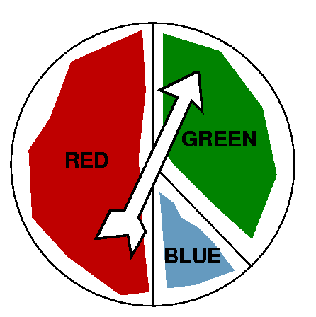
is 1/2, hits green is 1/3, and hits blue is 1/6.
Then I discussed playing games and fare entry fees. Suppose we have a
"spinner", that is, a circular piece of material with an arrow pivoted
to swing around the center. Half of the area is red, one-third is
green, and a sixth is blue. Then the chance that the spinner hits red
is 1/2, hits green is 1/3, and hits blue is 1/6.
This is a very complicated statement. The estimate for |R_N(x)|
actually has 4 different algebraic variables: x and c and N and
M_{N+1}.
The reason why the theorem is true is not straightforward. The text
has one method. I prefer to use a technique involving integration by
parts, a method similar to what I indicated was used for estimating
the error in various integration approximation techniques. In this,
int_c^x f'(t)dt=f(x)-f(c), and the parts are u=f'(t), dv=dt, and
du=f'(t)dt and v=the non-obvious t-c. I didn't pursue this, but it
really does work.
This is a very complicated statement. The estimate for |R_N(x)|
actually has 4 different algebraic variables: x and c and N and
M_{N+1}.
To see that the theorem is true is not straightforward. The text
has one method. I prefer to use a technique involving integration by
parts, a method similar to what I indicated was used for estimating
the error in various integration approximation techniques. In this,
int_c^x f'(t)dt=f(x)-f(c), and the parts are u=f'(t), dv=dt, and
du=f'(t)dt and v=the non-obvious t-c. I didn't pursue this, but it
really does work.
Go to the old dead tree at dawn. Then at sunrise, walk ten paces in a
north-north-east direction from the tree. Dig there for treasure.