Math 421 diary, fall 2005
Partial Differential Equations and Boundary Value Problems
I "reviewed" the two-dimensional heat equation on the Pi-by-Pu
square. We discussed the Steady State and Transient solutions, both
qualitatively (flow lines, isothermals, etc. and -->0 for steady
state) and quantitatively (the formulas involving trig/hyperbolic
series for the Dirichlet problem, and involving double sine series for
the transient solution).
Waving
A thin plate made of homogeneous material vibrating with no friction
(no dissipation) would move according to the two-dimensional wave
equation:
utt=uxx+uyy. A simple
boundary value problem for this PDE on the Pi-by-Pi unit square
is:
(PDE) utt=uxx+uyy.
(BC) u is zero on all of the boundary all of the time: that is,
u(x,0,t)=0 and u(x,Pi,t)=0 for all x in [0,Pi] and
u(0,y,t)=0 and u(Pi,y,t)=0 for all y in [0,Pi].
(IC) Here both an initial position (displacement) and velocity will be
specified: u(x,y,0)=J(x,y) and ut(x,y,0)=K(x,y).
The boundary condition of course corresponds to the edges of the
square plate somehow fixed to the equilibrium position. This is a
rather simple boundary condition. Boundary conditions for the wave
equation can be much more complicated. In particular, the BC here is
not what is called a clamped plate which is important in
practice. That problem is much more complicated.
The additional information in the initial conditions satisfies the
physical "intuiion" that the motion of an object should depend on two
initial conditions (position and velocity). Also, from the
mathematical point of view, the PDE is second order in time, t, and
initial value problems for such equations need two chunks of
information. When we try initial data like sin(3x)sin(8y)FUNC(t),
which satisfies all the (BC)'s, then
FUNC´´(t)=-[32+82]FUNC(t) if we want
the wave equation to be true. Thus FUNC(t) should be a linear
combination of sin(sqrt(32+82)t) and
cos(sqrt(32+82)t).
Just J
Let's look for u(x,y,t) satisfying
(PDE) utt=uxx+uyy.
(BC) u is zero on all of the boundary all of the time: that is,
u(x,0,t)=0 and u(x,Pi,t)=0 for all x in [0,Pi] and
u(0,y,t)=0 and u(Pi,y,t)=0 for all y in [0,Pi].
(IC) u(x,y,0)=J(x,y)=sin(3x)sin(8y) and
ut(x,y,0)=K(x,y)=0.
FUNC is
a function chosen to be 1 at t=0 and to have derivative 0 at t=0. Also
its second derivative should almost be itself. We hesitated for a
while and then, in a dramatic display of delayed competence, we
asserted:
u(x,y,t)=sin(3x)sin(8y)cos(sqrt(32+82)t)
You can (you should!) check this. By now, though, you should
appreciate that everything is chosen to work out correctly. Two
derivatives of cos(sqrt(32+82)t) will "spit out"
two copies of sqrt(32+82) and a minus sign, and
this is exactly what uxx+uyy does to
u(x,y,t). Wonderful!
Additionally, the t part shows that the plate vibrates up and down,
just as we could imagine an ideal plate would behave.
and now K alone
Let's look for u(x,y,t) satisfying
(PDE) utt=uxx+uyy.
(BC) u is zero on all of the boundary all of the time: that is,
u(x,0,t)=0 and u(x,Pi,t)=0 for all x in [0,Pi] and
u(0,y,t)=0 and u(Pi,y,t)=0 for all y in [0,Pi].
(IC) u(x,y,0)=J(x,y)=0 and
ut(x,y,0)=K(x,y)=sin(44x)sin(83y).
Let's just write the answer:
u(x,y,t)=sin(44x)sin(83y)cos(sqrt(442+832)t)
Again, I don't think that this is too surprising after all of our
experience. You could go back and consider the one-dimensional
formulas again, and check that they are gotten using the same ideas.
Together? Does linearity ever stop?
So now
(PDE) utt=uxx+uyy.
(BC) u is zero on all of the boundary all of the time: that is,
u(x,0,t)=0 and u(x,Pi,t)=0 for all x in [0,Pi] and
u(0,y,t)=0 and u(Pi,y,t)=0 for all y in [0,Pi].
(IC) u(x,y,0)=J(x,y)=135sin(3x)sin(8y) and
ut(x,y,0)=K(x,y)=-403sin(44x)sin(83y).
The solution is
u(x,y,t)=135sin(3x)sin(8y)cos(sqrt(32+82)t)-403sin(44x)sin(83y)cos(sqrt(442+832)t)/sqrt(442+832)
and I might write in class on the board the word, Clearly! and this is almost true if you have
followed the discussion.
I wrote an answer out in disgusting detail in termms of the double
Fourier sine series of what is called here J(x,y) and K(x,y).
Conservation of energy with this wave equation
Diary entry in progress! More to
come.
 One more detail
But it isn't a tiny detail. We've just seen how to solve what are called
initial value problems with zero boundary data provided that the
initial conditions are given as linear combinations of
sin(n x)sin(m y) with n and m positive integers. But what if
there aren't any natural expressions for the initial data? Look at the
following:
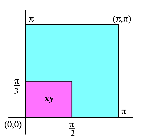
Suppose J(x,y) is xy when x is between 0 and Pi/2 and when y
is between 0 and Pi/3. Otherwise J(x,y) is 0.
To use the methods we discussed above, we need to represent J(x,y) as
a sum of constants multiplying
sin(n x)sin(m y) with n and m positive integers. How can we
do this?
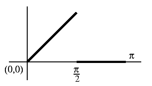 Well I just happen to know that if we take the function
J1(x), defined by J1(x)=x for x in [0,Pi/2] and
0 otherwise, then
J1(x)=SUMn=1infinityansin(n x)
where
an=(2/Pi)
Well I just happen to know that if we take the function
J1(x), defined by J1(x)=x for x in [0,Pi/2] and
0 otherwise, then
J1(x)=SUMn=1infinityansin(n x)
where
an=(2/Pi) 0PiJ1(x)sin(n x)dx=(2/Pi)0Pi/2x·sin(n x)dx
(hey, I could compute that if I wanted to, but I've already done 205
integrations by parts in this course).
0PiJ1(x)sin(n x)dx=(2/Pi)0Pi/2x·sin(n x)dx
(hey, I could compute that if I wanted to, but I've already done 205
integrations by parts in this course).
 y stuff
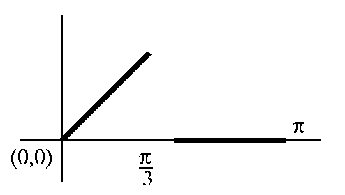
Well I just happen to know that if we take the function
J2(y), defined by J2(y)=y for y in [0,Pi/3] and
0 otherwise, then
J2(y)=SUMm=1infinitybmsin(m y)
where
bm=(2/Pi)0PiJ2(y)sin(m y)dy=(2/Pi)0Pi/3y·sin(m y)dy
(and I'm not going to do this computation either).
So we have the Fourier sine series for J1 and
J2. If we multiply the two series and notice (!) that
J(x,y)=J1(x)J2(y), then
J(x,y)=SUMn,m=1infinityanbmsin(n x)sin(m y)
This is a double Fourier sine series for J(x,y) and if we
had to (!) we could now solve (or approximate solutions of) the
PDE's we just looked at.
Double sine series
Suppose that J(x,y) is defined on the square with x and y between 0
and Pi. Compute
cnm=(4/Pi20Pi0PiJ(x,y)sin(n x)sin(m y)dxdy
Then J(x,y)"="SUMn,m=1infinitycnmsin(n x)sin(m y)
This is called the double Fourier sine series for J(x,y). The
(4/Pi2) comes from squaring the one-dimensional
normalization constant 2/Pi. The reason for the quotes around the
equal sign is that this Fourier expansion has the same defects and
virtues as the one-dimensional example. For J(x,y) you are likely to
see, the expansion will converge to J(x,y) except maybe on a very
small collection of points in the square, and you would have to be
very unlikely (or be in a math course [maybe that's the same!]) to
even observe the difference.
One last example
Here is a slightly more complicated example than the xy function I
started with. I began this example in class. I cheated with the xy
function because I got the double sine series as a product of two
one-dimensional sine series. But what if I wanted a double sine series
for, say, a function like J(x,y) which equals x+y when x+y is between
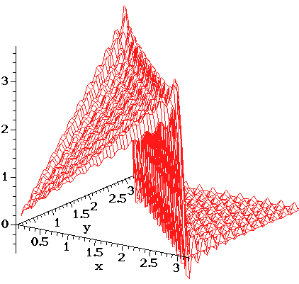
0 and Pi and which is 0 otherwise. Let me try to use Maple on
this function. The function is a tilted plane over a triangular region
in the xy-plane, and is 0 otherwise. As you can see, Maple
does not handle the two-dimensional discontinuities of the function
nicely. I don't know how to fix that. | 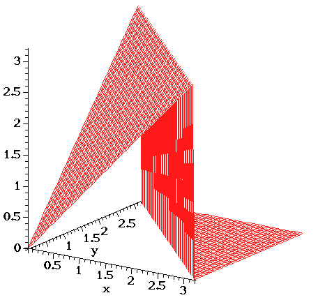
|
|
I wrote Maple commands to compute the two-dimensional Fourier
sine coefficients for this function, and then assemble these
coefficients and the appropriate sine functions into a partial sum of
the two-dimensional Fourier sine series. I had Maple graph
a partial sum.
Plotting this function took a lot of time. The 25th partial
sum has 252=625 Fourier coefficients, and then I asked that
the plot be done on a 50-by-50 grid (2500 evaluations). I did
cheat a little bit. If you examine the plot instruction closely
(the instruction is written below), you will see that I had the
partial sum plotted on the square whose sides both run from .01 to Pi,
and not from 0 to Pi. That's because there is horrible misbehavior of
the graph near the boundary, since this is a graph of sines, and the
boundary values all have to be 0. Additionally, there is Gibbs
bouncing around on these borders. You can still see some of the Gibbs
stuff in the graph here, though. I tried the graph from 0 to Pi on
each side, and the shape of the graph away from the edges was
difficult to see.
|
|
Here are the Maple commands I used.
The plot3d function is part of the package plots and
one way of using it is to type with(plots): earlier in the
Maple session.
>f:=(x,y)->evalf(piecewise((x+y<Pi),(x+y),0));
>a:=(n,m)->evalf((4/Pi^2)*int(int(f(x,y)*sin(n*x)*sin(m*y),x=0..Pi),y=0..Pi));
>T:=(N,x,y)->add(add(a(n,m)*sin(n*x)*sin(m*y),n=1..N),m=1..N);
>plot3d(T(25,x,y),x=.1..Pi,y=.1..Pi,axes=normal,style=hidden,color=N,grid=[50,50],orientation=[-56,74]);
HOMEWORK
Come to review sessions if you can:
Wednesday, December 14 at 4-6 PM in Hill 425
Laplace transforms
& linear algebra.
Thursday, December 15 at 4-6 PM in Hill 425 Fourier series, the
wave/heat equations, & associated boundary value problems.
and
please come to the final exam:
Math 421:01, Friday, December 16, 8 AM-11 AM, SEC 216
| What every child should know about
trig and hyperbolic functions ... |
|---|
TRIG
onometric |
cosine | cos(0)=1
cos´(0)=0 |
y´´=-y | cos(t)=([eit+e-it]/2)
| It wiggles between -1 and 1
always | 
|
|---|
| sine | sin(0)=0
sin´(0)=1 |
y´´=-y | sin(t)=([eit-e-it]/2i) |
It wiggles between -1 and 1 always | 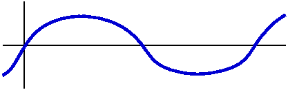 |
HYPER
bolic |
cosh | cosh(0)=1
cosh´(0)=0 |
y´´=y | cosh(t)=([et+e-t]/2)
| It gets big both ways
both sides are + |
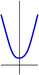 |
|---|
| sinh | sinh(0)=0
sinh´(0)=1 |
y´´=y | sinh(t)=([et-e-t]/2) |
It gets big both ways
+ on the right; - on the left |
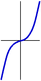 |
 Let's try to do some two dimensional problems. I'll try the heat
equation first. Consider a thin homogeneous object, lying over a
region R in the plane. The same analysis as we went through for heat
in a bar will work here: Newton's law of cooling, heat proportional to
temperature, etc. If u(x,y,t) is the temperature at a point (x,y) in
the region R at time t, then (setting all the physical constants equal
to 1, again, which should irritate those who live in the real world!),
we have ut=uxx+uyy. This is the
two-dimensional heat equation. Again just setting up a good problem to
study takes some preparation. There will be the (PDE) and certain
(BC)'s, boundary conditions, and, of course, an initial condition,
(IC). One arrangement which has been studied and might be useful in
the "real world" is the following:
Let's try to do some two dimensional problems. I'll try the heat
equation first. Consider a thin homogeneous object, lying over a
region R in the plane. The same analysis as we went through for heat
in a bar will work here: Newton's law of cooling, heat proportional to
temperature, etc. If u(x,y,t) is the temperature at a point (x,y) in
the region R at time t, then (setting all the physical constants equal
to 1, again, which should irritate those who live in the real world!),
we have ut=uxx+uyy. This is the
two-dimensional heat equation. Again just setting up a good problem to
study takes some preparation. There will be the (PDE) and certain
(BC)'s, boundary conditions, and, of course, an initial condition,
(IC). One arrangement which has been studied and might be useful in
the "real world" is the following:
(PDE) u satisfies the two-dimensional heat equation,
ut=uxx+uyy.
(BC) We prescribe the boundary temperature for all time for points,
(x,y), on the boundary of R.
(IC) We give an initial temperature distribution, u(x,y,0), for all
points (x,y) inside R.
This works. It's turns out to be what's called a "well-posed boundary
value problem". There's exactly one solution, and it has properties
which are expected from physical models. And, again, the solution
turns out to be the sum of a transient solution depending more or less
on the (IC) and a steady-state solution, which really depends on the
(BC)'s. The steady state solution has no dependence on time. In the
one-dimensional case, with ut=uxx, solutions
which don't depend on time just solve uxx=0. So these
functions are Ax+B for constants A and B. We can understand these
well. Geometrically their graphs are just straight lines. For
example, they are simply and totally determined by the correct
combination of temperatures at the end of the rod or by insulating
conditions.
More complicated things occur in two dimensions. I will try to study
just one steady-state solution to give an example. In two dimensions,
with ut=uxx+uyy, if there is no t in
the u function, then the equation
uxx+uyy=0
must be satisfied. This is called
Laplace's equation. I remarked that 6x2-5y+44xy-12t
was a solution to Laplace's equation, and we checked this by
differentiating. I then said, "So what?" By that I meant that I wanted
to find physically meaningful solutions of Laplace's equation. For
this I need (BC)'s. I don't need initial conditions, since there is no
t in this problem.
I'll look at a very simple choice of region R in the plane. In the
plane, this usually means one of two domains: either the inside of a
circle (a disc) or a rectangular region. Studying the disc introducing
the complications of Bessel's equation. You should know about Bessel's
equation (see chapter 15), but I won't tell you. I will instead choose
the somewhat simpler rectangular region.
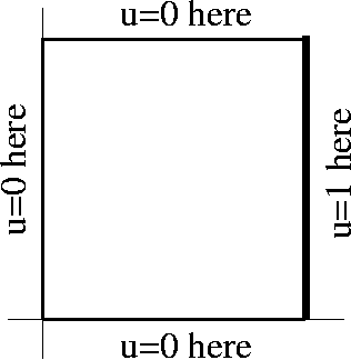 Here is the boundary value problem I want to study:
(PDE) u satisfies the two-dimensional heat equation,
uxx+uyy=0 for x and y between 0 and Pi.
(BC) The boundary temperature is 0 when y=0 and y=Pi and x=0, and it
is 1 when x=1. A picture is really good here.
This should be enough information to determine a unique steady-state
solution. What should this steady-state solution "look like"? I hope
that class discussion will suggest:
- The temperature range on the inside will always be between 0
and 1.
- Close to the edge with temperature 1, the temperatures should be
close to 1. Close to the other edges, the temperatures should be close
to 0.
- There should be no interior maximums or minimums to the
temperature (this is steady-state, and otherwise there would be heat
flow and there is no reason for spontaneous lumps of heat to form
inside the plate).
- The temperature graph should be really smooth: no jumps, no
creases or shocks. Just smooth, locally averaging again.
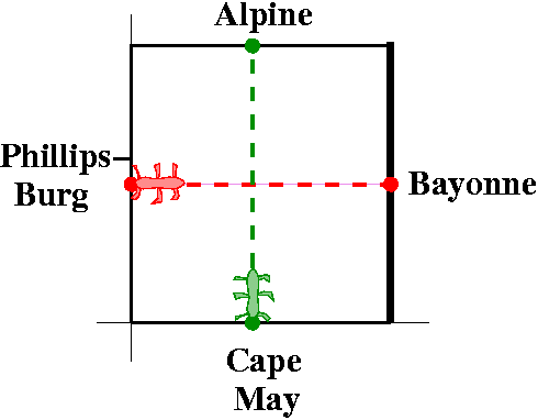 Additionally, we might think of two ants, crawling say from left to right
and from down to up.
Additionally, we might think of two ants, crawling say from left to right
and from down to up.
From Phillipsburg to Bayonne, I would expect the temperature to
increase from 0 to 1. I don't know much more than that.
From Cape May to Alpine, I would expect the temperature to increase
from 0 to a maximum and then back down to 0. The max would of course
be something less than 1. And I would expect the graph to be symmetric
about 1/2.
This is all nice and qualitative, but an engineer might also want
numbers: what the heck is the temperature at, say, (1,2)? So
I'd like to at least roughly check the qualitative predictions, and
get some guess about u(1,2).
Consider uxx+uyy=0 and separate variables. Now
we will guess that u(x,y) is X(x)Y(y), and Laplace's equation becomes
X´´(x)Y(y)+X(x)Y´´(y)=0 or Y´´(y)/Y(y)=-X´´(x)/X(x). Again, this must
be a constant. I'll call the constant, C.
What is Y(y)?
So we've got Y´´(y)=CY(y). The boundary conditions at y=0 and y=Pi are
0.
What if C=0?
Now the solutions of Y´´(y)=0 are Ay+B. If Y(0)=0
then B=0. If Y(Pi)=0 then A=0. So this solution is only the
identically 0 solution, which is not of much help in finding a
non-zero product solution.
What if C>0?
The solutions of Y´´(y)=CY(y) are the linear combinations of
sinh(sqrt(C)y) and cosh(sqrt(C)y). Thus
Y(y)=Asinh(sqrt(C)y)+Bcosh(sqrt(C)y). Since Y(0)=0, we know that B=0
(since sinh(0)=0 and cosh(0)=1). The Pi boundary condition gives
Bcosh(sqrt(C)Pi)=0 so B must be 0.
We're left with C<0.
I guess I should rename C: it will be - 2. The solutions
of Y´´(y)=-2Y(y) are then Asin(y)+Bcos(y). The
boundary condition Y(0)=0 means that B must be 0. The boundary
condition Y(Pi)=0 means that sin(Pi)=0. We know (repetition is the
foundation of learning?) that is a a positive integer, which we
will call n.
2. The solutions
of Y´´(y)=-2Y(y) are then Asin(y)+Bcos(y). The
boundary condition Y(0)=0 means that B must be 0. The boundary
condition Y(Pi)=0 means that sin(Pi)=0. We know (repetition is the
foundation of learning?) that is a a positive integer, which we
will call n.
So now -2 is -n2 and Y(y)=sin(n y).
What is X(x)?
We know Y´´(y)/Y(y)=-X´´(x)/X(x) and our analysis of the separation
constant for Y(y) shows that -X´´(x)/X(x)=-n2, so that we
need to consider X´´(x)=n2X(x): a positive
number. Be careful! Things are more complicated now because the
separation constant has suddenly turned positive. Therefore
X(x)=Asinh(n x)+Bcosh(n x). X(0)=0 forces B to be 0. So the
function must be sinh(n x).
Building up from the product solutions by superposition
Now we know that sinh(n x)sin(n y) is a solution to
Laplace's equation for each positive integer n. You can check
this as we did in class by finding two x derivatives and two y
derivatives. n2 comes out in each case because the chain
rule acts on sinh and on sin, and the yy derivative has a minus sign,
while the xx derivative has a plus sign.
We take linear combinations, since Laplace's equation is linear. A
solution u(x,y) is, therefore,
SUMn=1infinityvnsinh(n x)sin(n y)
and we don't know what the numbers vn are. But, wait, we
have not used the last boundary condition: u(Pi,y)=1. The sum is then
constrained. Plug in x=Pi and get:
SUMn=1infinityvnsinh(n Pi)sin(n y)=1.
This means, as a function of y, the Fourier sine series of 1 should be
equal to a sine series whose coefficients are
vnsinh(n Pi). But the coefficients of the Fourier sine
series of 1 are
[2/Pi]0Pi1·sin(nx) dx. So
vn must be
[2/{Pi sinh(n Pi)}]0Pi1·sin(nx) dx.
These are lots of numbers. We can compute the integrals, and either by
hand or with Maple guess at what they are. It turns out that
for even n's the integrals are 0 (all the sine bumps cancel) and for
odd n's the integrals are 4/(nPi). So the solution as explicitly as I
can conveniently write it seems to be:
SUMn=1
infinity(4/[{2n+1} Pi sinh({2n+1}Pi)])sinh({2n+1} x)sin({2n+1} y)
ODD INTEGERS ONLY because the even sine Fourier
coefficients of 1 are 0.
What about the sinh numbers? 1/sinh(n Pi) is about
2e-n Pi and for n large this is very small. So the
series converges fast. I did some experiments with the first 50
or so terms.
The graphs exhibited below are from the class handout. There's a graph of the
surface z=u(x,y), and also showed the contour lines. The graph and the
contour lines near the corners where the boundary values 0 and 1 meet
are sort of a mess and hard to understand, and even hard to picture
and compute. The contour lines in this case are traditionally called
isothermals, lines of constant temperature. We also saw that the trip
from Phillipsburg to Bayonne did go from 0 to 1. Maybe (?) it is clear
to some people why this graph is concave up. The trip from Cape May to
Alpine is as predicted qualitatively. I even evaluated u(1,2) and got
the approximation .1176183537. Because of the rapid growth of sinh,
I'm sure this is quite accurate.
| The surface is a graph of u(x,y) |
The contour lines (isothermals) of u(x,y) |
|---|
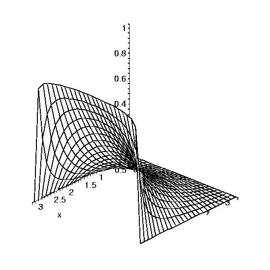 |
 |
| From Cape May to Alpine |
From Phillipsburg to Bayonne |
|---|
 |
 |
And in general?
It isn't too hard to see how everything would work if we replaced 1 on
the boundary by some function of y. We would just compute the Fourier
sine coefficients, multiply by the appropriate
[2/{Pi sinh(n Pi)}], add, etc. Here we go:
(PDE) Laplace's equation: uxx+uyy=0.
(BC)u(x,0)=0 and u(x,Pi)=0 and u(0,y)=0 and u(Pi,y)=Q(y), where Q(y)
is some weird function of y.
I think the solution will look like
u(x,y)=SUMn=1infinityvnsinh(n x)sin(n y)
where the coefficients are obtained as slight modifications of
the Fourier sine coefficients of Q(y): vn=[2/{Pi sinh(n Pi)}]0PiQ(y)·sin(nx) dx.
The sin(n y) comes from the zero boundary conditions on the top
and bottom of the square. The zero boundary condition on the left,
together with the + sign in Laplace's equation give a positive
separation constant, and therefore sinh(n x). Finally, the
formula for vn gives me the righthand boundary condition.
Now we sat and thought a while. I suggested that we could equally well
solve similar boundary value problems where three edges were 0 and
some sort of function was specified along the other edge. A picture of
the situation is shown below.
The Dirichlet problem
If we can solve these separate problems, then we could solve the
Dirichlet problem, which is probably the single most important
and most basic boundary value problem in all of partial differential
equations (Google has more than 45,000 references for
"Dirichlet problem"):
(PDE) uxx+uyy=0 (Laplace's equation)
(BC) Boundary values for u are specified on all of the boundary.
There's no initial conditions here, because time doesn't come into it.
The method outlined above would allow you to solve this problem in the
square, or, at least, find a good approximation to the solution. If
accuracy is important, using software that's been previously used and
validated is probably a good idea! But if you wanted to do it
yourself, you could divide up the problem into 4 subproblems, and
solve each of them as we did the first, and then use linearity
and add up the solutions. Since the boundary data is 0 in lots of
places, summing the solutions won't harm the boundary values you
already have. So we can get steady-state heat flows, and by taking
partial sums of the series, we can even approximate these solutions
quite well.
And now for transient solutions
Suppose we want to solve the heat equation on the Pi-by-Pi square, but
now we specify initial data. Here is the problem I would like to
solve:
(PDE) ut=uxx+uyy. Here u is a
function of x and y and t, u(x,y,t). The PDE is called the
two-dimensional heat equation (the dimension count refers to
the number of space dimensions, which confuses me).
(BC) u is zero on all of the boundary all of the time: that is,
u(x,0,t)=0 and u(x,Pi,t)=0 for all x in [0,Pi] and
u(0,y,t)=0 and u(Pi,y,t)=0 for all y in [0,Pi].
(IC) There is an initial heat distribution, J(x,y), defined for
(x,y) in the square (x and y are both in the interval [0,Pi]),
and we want u(x,y,0)=J(x,y).
By the way, what are our "physical" expectations (?) for this
solution, a transient temperature distribution? I think that if
we hold the temperature at 0 on all of the boundary, we should expect
that rather rapidly the temperature distribution inside the plate
should --> 0 as t --> infinity. So we should check that our
mathematical model does this.
Simple, always simple ...
I tried to find some simple solutions to the boundary value problem
with an initial condition. We wanted a function J(x,y) which
satisfied the boundary conditions. So our initial J(x,y) was something
like sin(4x)sin(17y). This is not too wild a guess, since sine at
integer multiples of Pi is 0, and we need boundary values equal to 0
at 0 and Pi. Now what should u(x,y,t) be? The
simplest guess is that u(x,y,t) should be sin(4x)sin(17y)
multiplied by FUNC(t), some function of t. So I would like to try
u(x,y,t)= sin(4x)sin(17y)FUNC(t). What should be true about FUNC(t)?
If we want (IC) to be true, then certainly FUNC(0)=1. We can easily
compute uxx+uyy. The result will be
-(42+172)sin(4x)sin(17y)FUNC(t). And what about
ut? It should be sin(4x)sin(17y)FUNC'(t). For things to
agree, and for the heat equation to have a solution, we need
FUNC'(t)=-(42+172)FUNC(t) with FUNC(0)=1.
You should recognize this ordinary differential equation.
But not too simple ...
Hey. I now know the solution:
u(x,y,t)=sin(4x)sin(17y)e-(42+172)t.
The pieces all work together. It is not an accidental mess, but
carefully "guessed" or assembled or something. Now that we have an
idea, we shnould exploit it further. For example, we could try to
solve the BVP (boundary value problem)
(PDE) ut=uxx+uyy
(BC) u is zero on all of the boundary all of the time: that is,
u(x,0,t)=0 and u(x,Pi,t)=0 for all x in [0,Pi] and
u(0,y,t)=0 and u(Pi,y,t)=0 for all y in [0,Pi].
(IC) u(x,y,0)=J(x,y)=-3sin(6x)sin(8y)+9sin(11x)sin(42y)
Then the solution is
u(x,y,t)=-3sin(6x)sin(8y)e-(62+82)t+9sin(11x)sin(42y)e-(112+422)t.
I am using linearity (the principle of superposition) together with
our wonderful idea about creating a companion exponential which
when multiplied together with the sine/sine initial conditions will
solve the heat equation. Also you should notice that the negative
signs in the arguments of the exponentials drive down the amplitudes
of the initial heat distribution. More mathematically, as
t-->infinity, u(x,y,t)-->0 as we guessed earlier.
I then tried to indicate (not describe precisely) how we could solve
the whole mess:
(PDE) ut=uxx+uyy
(BC) u is specified on all of the boundary all of the time: that is,
u(x,0,t)=S(x) and u(x,Pi,t)=P(x) for all x in [0,Pi] and
u(0,y,t)=R(y) and u(Pi,y,t)=Q(y) for all y in [0,Pi].
(IC) There is an initial heat distribution, J(x,y), defined for
(x,y) in the square (x and y are both in the interval [0,Pi]),
and we want u(x,y,0)=J(x,y).
First I would solve the Dirichlet problem for
uxx+uyy=0 with the indicated boundary
conditions. I would get some sort of steady-state solution, which I'll
call SS(x,y). Then I would solve the heat equation with zero boundary
conditions and with initial conditions equal to J(x,y)-SS(x,y). I
would add the solution of that problem to SS(x,y). Because of various
seros in boundary conditions, etc. (linearity again) the function of x
and y and t would actually solve the whole problem stated above. Of
course, I would hope that this could all be implemented by a properly
tested computer program. There are lots of details which an unassisted
human being could (would?) screw up.
For the initial condition, I would assemble a
Double sine series
Suppose that J(x,y) is defined on the square with x and y between 0
and Pi. Compute
cnm=(4/Pi20Pi0PiJ(x,y)sin(n x)sin(m y)dxdy
Then J(x,y)"="SUMn,m=1infinitycnmsin(n x)sin(m y)
This is called the double Fourier sine series for J(x,y). The
(4/Pi2) comes from squaring the one-dimensional
normalization constant 2/Pi. The reason for the quotes around the
equal sign is that this Fourier expansion has the same defects and
virtues as the one-dimensional example. For J(x,y) you are likely to
see, the expansion will converge to J(x,y) except maybe on a very
small collection of points in the square, and you would have to be
very unlikely (or be in a math course [maybe that's the same!]) to
even observe the difference.
HOMEWORK
1. Please give me on Monday, the next (and last) class a sheet of
paper with all of your homework grades and your name. Some of the
homework grades have been misplaced and I want to give people all the
credit they deserve.
2. I handed out a sheet of homework problems on
two dimensional PDE's. You may try these yourself. Answers to these
questions and to some questions from the textbook are given here.
3. Our final exam is on Friday, December 16, from 8 to 11 AM in SEC
216, our usual classroom. Review sessions are scheduled as
follows:
Wednesday, December 14 at 4-6 PM in Hill 425
Laplace transforms
& linear algebra.
Thursday, December 15 at 4-6 PM in Hill 425
Fourier series, the wave/heat equations, & associated boundary value
problems.
4. Please also see here for more review
material.
The instructor made a number of silly mistakes. No one can equal his
ineptitude when he gets going!
Here is the solution to the the wave equation:
(PDE) The wave equation: uxx=utt
(BC) u(0,t)=0 and u(Pi,t)=0 for all t.
(IC) u(x,0)=f(x) for x between 0 and Pi (initial position) and
ut(x,0)=g(x) for x between 0 and Pi (initial velocity)
has solution u(x,t)=SUMn=1infinitycnsin(nx)cos(nt)+SUMn=1infinitydnsin(nx)sin(nt).
where
cn=(2/Pi)0Pif(x)sin(nx) dx
and
dn=[2/(nPi)]0Pig(x)sin(nx) dx.
We need the n's in the dn formula because that part deals
with a derivative initial condition, and the n's make things work out
correctly. As I remarked in class, this is wonderful. Well, maybe it
is. If you are given f(x) and g(x) and you need to compute u(.2,.7),
then you certainly can get a good approximation using the solution
above. But it turns out that there are other ways of looking at the
solution which are very useful. These other ways are already in the
pictures, if you look closely. I tried to motivate the other ways
algebraically by looking at, say, sin(nx)cos(nt), which is a piece of
one of the sums.
Look at the Fourier solution again ...
Trig identities tell me that
sin(nx)cos(nt)=(1/2)sin(nx+nt)+(1/2)sin(nx-nt). Now this is
(1/2)sin(n(x+t))+(1/2)sin(n(x-t). A similar result is true for
sin(nx)sin(nt). You could imagine that we then
reassemble the infinite sums and separate them, with one chunk
involving x-t and one chunk involving x+t. Huh. So let's try
"something completely different" (quoted from Monty Python).
Make a guess
Suppose Func and Otherfunc are two functions of one variable. Then
consider the function
u(x,t)=Func(x-t)+Otherfunc(x+t)
.
The chain rule tells me that
ux(x,t)=Func´(x-t)(1)+Otherfunc´(x+t)(1)
and I can't write more than that since I haven't told you much about
Func and Otherfunc. But I will differentiate again with respect
to x:
uxx(x,t)=Func´´(x-t)(12)+Otherfunc´´(x+t)(12)
These computations will get somewhere, soon. Because we now try things
with respect to t:
ut(x,t)=Func´(x-t)(-1)+Otherfunc´(x+t)(1)
and most important, notice the -1 which happens when the chain rule,
differentiating with respect to t, meets x-t. But now the
second t derivative:
utt(x,t)=Func´´(x-t)(-1)2+Otherfunc´´(x+t)(12)
Since -1 squared is 1, well, golly, we have found solutions of
uxx=utt.
 Waves moving
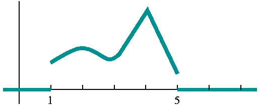
What's going on? Well, I then tried to draw some silly
pictures. Suppose I give you only graphical information about
Func. Its graph is as shown to the right. So Func is 0 when its input
is less than 1 or greater than 5, and in between it has the strange
profile shown.
What will Func(x-t) look like for various times? Well, we discussed
this and below is the result of sketching Func(x-t) when t=0 and t=1
and t=2. Please look carefully at the numbers on the horizontal axes.
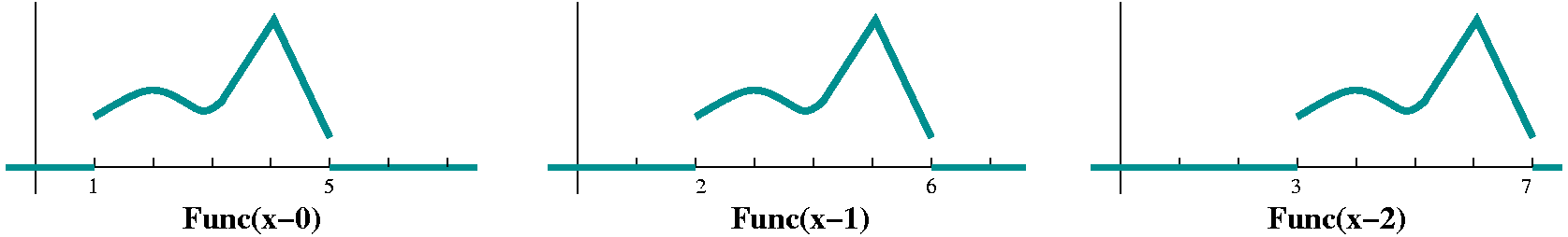
Apparently Func(x-t) is really a wave which is moving to the right. A
similar analysis shows that Otherfunc(x+t) is a wave moving
left. Maybe I should relabel these pieces, and we see that this is a
solution of the wave equation:
u(x,t)=Right(x-t)+Left(x+t)
This is the D'Alembert form of the solution to the wave
equation. I think I now introduced another classic parameter of the
wave equation, a positive number called c, which will be the speed of
propagation of the waves (in context, this could be, for example, the
speed of light or the speed of sound or ... lots of things). Then
consider the function
u(x,t)=Right(x-ct)+Left(x+ct)
It turns out that this function satisfies the wave equation with a
slight change:
c2uxx=utt
Problems 13 and 14 of section 13.4 of the text discuss the D'Alembert
solution and even give the following relationship between the initial
position/velocity solutions:
If u(x,0)=f(x) and ut(x,0)=g(x), then
u(x,t)=(1/2)[f(x+ct)+f(x-ct)]+[1/(2c)] x-ctx+ctg(s)ds.
I don't believe that you need to memorize many of these formulas. You
should know that they are around, though. If you look at the pictures
which were distributed and look at the moving
images, I think you should be able to guess at the left and right
traveling waves.
| Qualitative comparison of solutions
to the wave and heat equations |
|---|
| | Behavior for large time |
Speed of propagation |
Rough vs. smooth |
Reversibility |
|---|
| Solutions of the heat equation |
The solutions are sums of transient and steady-state. Here (BC)'s
give different steady-state solutions. (IC)'s give transient solutions
which decay rapidly with time so that long term solutions are very close to
steady-state. |
In this model, speed seems infinite, but effects are exponentially
small for small time as you move away from where the (IC)'s are not 0.
|
Even if (IC)'s are very rough, the heat equation averages, and so
for any positive time, even very small positive time, the
temperature is very smooth. |
Time can't be reversed: if u(x,t) is a solution to the heat
equation, u(x,-t) is rarely also a solution. Things don't
undiffuse: entropy increases. |
|---|
| Solutions of the wave equation |
This is idealized motion, and there is conservation of energy: no
dissipation. The solutions are all periodic, and there is no
equilibrium solution except for constants. |
There is a fixed propagation speed (in homogeneous media). |
Waves moving right and left can be very rough: there can be
shocks, and these shocks may persist. |
If u(x,t) solves the wave equation, so does u(x,-t) (because
(-1)2=1). Therefore a film run in reverse of a solution
of the ideal wave equation would also show a picture of a solution
to the wave equation. Solutions are reversible in time. |
|---|
Comments on colors should be directed to the Math
421 webmaster, Hieronymus Bosch.
The instructor discussed how to solve a homework problem. He didn't do
the computational parts.
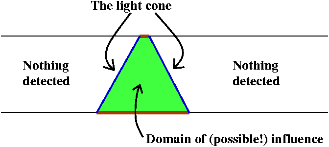 Light cones
Light cones weigh much less than heavy cones. Sorry. Back to work:
imagine a very long string, which is somehow held tight along the
x-axis. Suppose I tweak the string a little bit around a number x (I
change the position and/or the velocity). What could possibly happen
at later time? If you really "buy into" the D'Alembert form of the
solution, then you see that the information about the tweaking can't
be detected until the waves (moving left or right) get there.
The possible influence doesn't get felt outside of the interval
[x-ct,x+ct]. This is called the light cone. If you believe, really
believe, in special relativity, and so you think that the speed of
light is an absolute limit, then you can't signal faster than the
speed of light, so a person standing at x at time 0 can only influence
events at time t in the interval [x-ct,x+ct].
Well, the idea is important. So now you engineers have lots to
remember about the wave equation. There are Fourier series solutions,
D'Alembert's traveling wave solutions, the pictures, etc.: lots of
stuff.
I began the study of the two dimensional heat equation, which I will
continue next time.
HOMEWORK
Our final exam is on Friday, December 16, from 8 to 11 AM in SEC
216, our usual classroom. More information about the exam will
appear shortly.
Please do think about when a review session can be held, and when
office hours might be convenient.
The notes for the class follow, but also see here, please.
The basic assumptions for the
Wave Equation are described on pp. 693-4 of the textbook. I have been
sworn to and at by the Mech Engineering faculty who assert that they
will teach the derivation of the wave equation in their courses and I
should stay away. By the way, there are many nice descriptions of this
derivation on
the web. In any case, the wave equation models the motion of an
idealized string. We'll assume the string is stretched between two
points on the x-axis. I'll call the points x=0 and x=Pi (not a big
surprise!). We will assume that the motion of the string is
perpendicular to the x-axis, and stays in the xy-plane. The function
u(x,t) is supposed to model the height (displacement?) of the portion
of the string which is over the point x at time t. Then it turns out
that uxx=utt: this is the one-dimensional
wave equation. I have forced the physical constants to be 1. This
turns out to be a rather serious (and sometimes misleading!)
assumption, but I'll work with it for today since it will make some of
the algebra easier.
I should emphasize that this vibrating string is supposed to be ideal. So there is no friction, and everything
"works". As I said in class, it is probably a good idea to review a
much simpler model, the vibrating sPring (not sTring,
very easy to mispronounce for me!). Here is a discussion I wrote of
the standard model (Hooke's Law, F=ma, etc.) of the spring. It is
useful to note that a picture of the spring of any time doesn't have
complete information: both the position (in relation to equilibrium)
and the velocity of the spring must be considered. Also in this simple
model, these is also no friction, and so no dissapation of the energy:
energy is conserved, and this has very important consequences for the
spring. It never stops vibrating!
O.k., back to the string. The simplest boundary value problem for the
string has the ends fastened: u(0,t)=0 and u(Pi,t)=0 for all t. Then
we would expect to have the string vibrate, depending what the initial
condition(s) are.
So I will study the following boundary value problem:
(PDE) The wave equation: uxx=utt
(BC) u(0,t)=0 and u(Pi,t)=0 for all t.
(IC) Well, let me skip this for a second.
Now we separate variables: if u(x,t)=X(x)T(t), then
uxx=utt implies that X´´(x)T(t)=X(x)T´´(t) so
that X´´(x)/X(x)=T´´(t)/T(t). The standard logical dance
(is it
a function of t -- left-hand side says no
is it
a function of x -- right-hand side says no) shows that
this is a constant, called the separation constant.
It is not true that such constants always turn out to be negative if
they arise in physical problems: we'll see this next week. Last time
we analyzed this constant using "math": now let's look at some
physical reasoning. Hey: if T´´(t)=(a positive constant)T(t)
then T(t) would have exponential growth or exponential decay. This
does not fit our physical intuition, so a positive separation constant
should be rejected. If, by the way, this offends your sense of
mathematical propriety (!), then you can eliminate such constants using
strictly math reasoning. If the separation constant is 0, then, say,
X´´(x)=0, so X(x) is Ax+B and (because of the boundary conditions) A=0
and B=0: the string doesn't move at all. The situation is not very
interesting.
Word of the day: fret
One definition:
n.[Mus] each of a sequence of bars or ridges on the
finger-board of some stringed musical instruments (esp. the guitar) fixing
the positions of the fingers to produce the desired notes.
Another definition:
v. a. be greatly and visibly worried or distressed.
b. be irritated or resentful.
So the separation constant is negative, and, like the textbook, we
will call it -2. Therefore the PDE separates into these
two ODE's: X´´(x)=-2X(x) and
T´´(t)=-2T(t). I'll analyze X(x) first.
Since X´´(x)=-2X(x) we know that any solution X(x) must
be a linear combination of cos(x) and sin(x). The boundary
conditions now help us. When x=0 we should get 0, so there can be no
term with cos(x) (because this is 1 at 0 while the sine term is 0 at
0). When x=Pi, we also get 0, so sin(x)=0. Draw a picture of sine in
your head, and that should convince you that must be an
integer. Since sin(-v)=-sin(v), we can push a negative sign onto the
scalar multiplier. Therefore we learn that
For this boundary-value problem, the eigenvalues are all positive
integers, n, and the eigenfunctions are sin(nx).
What are the possible partners of sin(nx) in u(x,t)=X(x)T(t)?
Well, T´´(t)=-n2T(t) so that T(t) must be a linear
combination of sin(nt) and cos(nt). Notice that both sin(nx)cos(nt)
and sin(nx)sin(nt) satisfy uxx=utt. You can
check this by direct differentiation! The principal of superposition
(linearity!) then applies. The solution u(x,t) must be a sum of two
kinds of terms (as just mentioned). So:
u(x,t)=SUMn=1infinitycnsin(nx)cos(nt)+SUMn=1infinitydnsin(nx)sin(nt).
Now we do need to discuss initial conditions. I put this off because
the initial conditions are more complex than with the heat
equation. Here an initial position is not enough. Go back and think
about the vibrating spring model again: a snapshot of where the spring
is does not have full information. We also need to know something
about the motion of the spring at the time to predict the future
behavior. Here we can specify both an initial position and an initial
velocity for the string.
We can specify these:
(IC) u(x,0)=f(x) for x between 0 and Pi (initial position) and
ut(x,0)=g(x) for x between 0 and Pi (initial velocity)
For simplicity, I will first study the case where g(x) is the zero
function (no velocity) and f(x) is specified (the initial
position). What happens now? If
u(x,t)=SUMn=1infinitycnsin(nx)cos(nt)+SUMn=1infinitydnsin(nx)sin(nt),
then
u(x,0)=b>SUMn=1infinitycnsin(nx)
since cosine is 1 at 0 and sine is 0 at 0. Thus
SUMn=1infinitycnsin(nx)=f(x) and
we should recognize this equation. The series is simply the Fourier
sine series for f(x), and the coefficients cn are given by
cn=(2/Pi)0Pif(x)sin(nx) dx. The
(2/Pi) is a normalization constant. But we also can get information
about the dn's. Since
u(x,t)=SUMn=1infinitycnsin(nx)cos(nt)+SUMn=1infinitydnsin(nx)sin(nt),
ut=SUMn=1infinitycnsin(nx)(-n) sin(nt)+SUMn=1infinitydnsin(nx)n cos(nt).
Since ut(x,0)=0 in our simple model, we get
SUMn=1infinitydnsin(nx)n=0.
But the functions sin(nx) are all linearly independent, and therefore
the dn coefficients are all 0. Hey!
We have solved (?) the boundary value problem:
(PDE) The wave equation: uxx=utt
(BC) u(0,t)=0 and u(Pi,t)=0 for all t.
(IC) u(x,0)=f(x) and ut(x,0)=0 for x between 0 and Pi.
The solution is
u(x,t)=SUMn=1infinitycnsin(nx)cos(nt)
where cn=(2/Pi)0Pif(x)sin(nx) dx.
So let's look at the velocity case:
(IC) u(x,0)=0 for x between 0 and Pi (initial position) and
ut(x,0)=g(x) for x between 0 and Pi (initial velocity).
Now we have
u(x,t)=SUMn=1infinitycnsin(nx)cos(nt)+SUMn=1infinitydnsin(nx)sin(nt).
When t=0, this becomes
SUMn=1infinitycnsin(nx) and if
this sum is 0, then (linear independence again) all of the
cn's are 0. But ut(x,t) is
SUMn=1infinitycnsin(nx)[-sin(nt)]n+SUMn=1infinitydnsin(nx)cos(nt)n.
Plug in t=0 and get
SUMn=1infinityndnsin(nx). So
we want
g(x)=SUMn=1infinityndnsin(nx).
Well, this is correct if ndn is the nth Fourier
sine coefficient of g(x). That is, if
dn=[2/(nPi)]0Pig(x)sin(nx) dx.
Does this solution give you all the intuition you would want? I don't
find it too comforting. Certainly, if you give me an initial profile
for the string, f(x), and an initial velocity, g(x), I could (maybe!)
compute the Fourier sine series coefficients. Then the wonderful
formulas above would allow me to predict the future behavior of the
string. Of course, in the real world, I would have to use partial
sums, get numerical approximations, etc.
Then we looked at some examples.
The first example
Here f(x) was a function which was
piecewise linear, 0 on [0,Pi/3] and [Pi/2,Pi], and had slope 1 on
[Pi/3,Pi/3+Pi/12] and had slope -1 on [Pi/3+Pi/12,Pi/2]: a sort of
little triangular tent, and g(x) was the 0 function We discussed what
how this initial data would evolve with the wave equation.
Here are some things we could see:
- The initial peak was actually a sum of two waves, one moving
right and one moving left.
- For later time, the waves kept their shape and their
non-differentiability ("shocks").
- When the waves hit the ends, the waves were reflected back upside
down.
- After an advance of 2Pi, the initial picture returned.
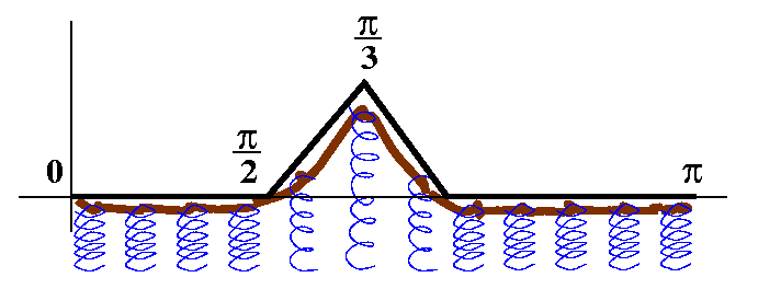 I tried to lead a discussion and convince people that these
observations predicted by the model actually could be seen
experimentally. Sigh. I even brought some string to class. The
qualitative aspects are very different from what happens in the
heat equation. It might help to think of the
string as sort of a mattress of springs tied together at the tops, but
each of them sort of behaving mostly like a Hooke's Law spring. This
is not a very good analogy. Oh well. The picture shown is supposed to
have "tiny" springs (in blue, if you can see the colors) tied together
by a thick brown string. The profile of the top of this "mattress" is
supposed to be like the f(x) which is in the handout. Oh well. The
middle of the bump moves down faster because the spring is stretched
more there. The springs at the edge pull up the nearby mattress
points. Oh well. Not a very good analogy, maybe.
I tried to lead a discussion and convince people that these
observations predicted by the model actually could be seen
experimentally. Sigh. I even brought some string to class. The
qualitative aspects are very different from what happens in the
heat equation. It might help to think of the
string as sort of a mattress of springs tied together at the tops, but
each of them sort of behaving mostly like a Hooke's Law spring. This
is not a very good analogy. Oh well. The picture shown is supposed to
have "tiny" springs (in blue, if you can see the colors) tied together
by a thick brown string. The profile of the top of this "mattress" is
supposed to be like the f(x) which is in the handout. Oh well. The
middle of the bump moves down faster because the spring is stretched
more there. The springs at the edge pull up the nearby mattress
points. Oh well. Not a very good analogy, maybe.
Wow! Now I tried to look with students at the second page of the handout. Here maybe we could imagine
that the string's initial position is 0 for all x, but that I have
given an impulse up to the portion of the string between Pi/3 and
Pi/2. I think this is slightly hard to imagine, but we discussed the
results anyway.
The first picture (for t=.1) shows that part of the string is moving
up. The tilted part of the profile, at the left and the right, shows
that the string is tied together (remember the mattress analogy: the
string is sort of made up of springs, but there's a tension between
adjoining "springs"). So there is resistence at the edge of the
impulse up. Then the effect begins to spread. At t=1.2, what I think
is a peculiar thing happens on the left. There are two tilted line
segments of slightly different slope. What is happening? Well, the
initial "up" hit the end of the string. We learned that the
profile is reflected down and fed back. The result in this case is
that the feedback of the wave front is subtracted from what is still
there, and we get the piecewise linear behavior. Something similar
happens on the right in the t=1.7 picture. The final picture, at t=3,
shows something very much like the initial behavior. But that is
correct, since when we increase t by 2Pi in the Fourier series, all of
the functions sin(nt) in the Fourier series have the same value:
sin(n(t+2Pi)=sin(nt+2nPi)=sin(nt). So u(x,t+2Pi)=u(x,t): this is
perfect, ideal wave behavior. There is no friction, no gravity, and no
energy dissipation
I find all this very difficult to understand. I asked if
some moving gifs would help, and was told, "Yes," so here they are.
HOMEWORK
I'll discuss the free boundary problem for the wave equation Monday,
as well as the D'Alembert solution for the wave equation (see problems
13 and 14 in section 13.4).
Please read sections 13.1--13.4 if you have not yet.
Please hand in (the last problems to hand in!) these problems:
13.3: 4
13.4: 3, 5
AND problem 9 from 13.4. I thank Mr. Clark for pointing out that I had already
assigned problem 1 in 13.3. I apologize.
I want to try another "physical" problem and see if this mathematical
model predicts what our intuition suggests.
Fixed (possibly non-zero) end temperatures
Now, again, let's have a bar overlaying the interval [0,Pi] whose
lateral ends are kept at specific temperatures. So the model looks
like this:
u(x,t) is the temperature at position x and at time t.
PDE The heat equation: ut=uxx
IC Initial condition: u(x,0)=f(x) for 0=<x<=Pi.
BC Boundary condition(s): u(0,t)=u0 and
u(Pi,t)=uPi.
Guessing long-term behavior
So what is the anticipated long-time behavior of these solutions?
Locally, the heat equation tries desperately to average
temperature as time progresses: if I am at position x, I will "feel"
positions x+(delta)x and x-(delta)x and try to update (?) my
temperature based on what's happening at those places compared to my
own. This means that the heat equation would urge (??) the long-term
temperature distribution to interpolated between the end temperatures
which are fixed. That is actually what the model will predict.
Let me assume some fixed values for u0 and
uPi. This will decrease the amount of algebra I'll need to
do. So I will assume that u(0)=2 and u(Pi)=5. There
are no particular vices or virtues about these numbers. They're just
convenient small integers.
Steady-state heat distributions
Suppose I seek functions, u(x,t), which satisfy the heat equation,
ut=uxx but which don't depend on time. Such
solutions would be called steady-state. If there is no time
dependence, then uxx=0. I know all the solutions of this
equation: Ax+B. These are straight lines. If I now want to have the
solution satisfy u(0,t)=2 and u(Pi,t)=5, then I compute (actually,
students computed!) that the steady-state solution should be
2+(5/Pi)x. The simplicity of this formula maybe is not something one
could have guessed from a verbal description of the mathematical
model. I might readily have guessed that the solution would increase
from to 2 to 5, but the precise shape of the curve (and details about
the formula) could well have been different.
Now here's a wonderful little trick to go from the "2 and 5" boundary
conditions to "0 and 0" boundary conditions. Suppose that u(x,t)
satisfies
PDE The heat equation: ut=uxx
IC Initial condition: u(x,0)=f(x) for 0=<x<=L.
BC Boundary condition(s): u(0,t)=2 and
u(Pi,t)=5.
Let's call the function 2+(5/Pi)x, SS(x). "SS" means "steady-state"
here. Then consider the function U(x,t)=u(x,t)-SS(x). What can we say
about U(x,t)? Since SS(x) and u(x,t) both satisfy the heat equation,
and the heat equation is linear, the function U(x,t), which is
a linear combination of u(x,t) and SS(x), also satisfies the heat
equation. What about the boundary conditions? Well, U(x,t) is assumed
to satisfy the "2 and 5" boundary conditions, and we know that SS(x)
satisfies the "2 and 5" boundary conditions, and these conditions are
linear. Therefore the difference satisfies the "0 and 0"
boundary conditions. Hey!
The U(x,t) function is a solution to the old problem. And we
know that the solutions to the old "0 and 0" problem all -->0 as
t-->infinity. This means that U(x,t)=u(x,t)-SS(x)-->0 so that
u(x,t)-->SS(x) as t-->infinity. This is exactly what we guessed should happen. So again this model predicts
the expected behavior.
Flux=0
The last situation I'd like to look was mentioned previously:
The setup Think of a bar with a certain distribution of
heat initially, and that somehow both ends of the bar are insulated:
no flow of heat is possible in or out of the ends. Maybe a diffusion
setup is simpler to understand here. We sprinkle (?) sugar into a tube
of water, and no further additions or subtractions to the tube are
made. Then we try to study how the concentration of the sugar
evolves. Presumably there is Brownian motion (caused by "random"
ambient heat) which moves things around.
The expected result Over a long time (a long, long time ...) I
would expect the sugar to be close to uniformly distributed in
concentration. There's no reason for lots of suger (or too little
sugar) to be in any one chunk of the tube: this would be remarkably
unlikely. So the concentration of sugar, u(x,t), would be close to
constant as t-->infinity.
I call this "Flux=0" because flux is another word for flow.
The mathematical model
Here is what we will work with:
PDE The heat equation: ut=uxx
IC Initial condition: u(x,0)=f(x) for 0=<x<=L.
BC Boundary condition(s): ux(0,t)=0 and
ux(Pi,t)=0.
We first will separate variables. This phrase is the name for
assuming that u(x,t) is a product function: X(x)T(t). The
result of using the PDE is then X´´(x)T(t)=X(x)T´(t). And then we get
X´´(x)/X(x)=T´(t)/T(t). This is now a constant, depending on neither x
nor t. What can happen?
The separation constant
There are several possibilities.
Irving The separation constant is positive.
Jessica The separation constant is zero.
Thrag The separation constant is negative.
What happens if we assume Irving? Well, then
T´(t)=(positive #)T(t), so that
T(t)=(const)e(positive #)t. I think that this is
physically unlikely: the temperature can't just increase and increase
(in this model heat is neither created nor destroyed inside the rod --
other, more complicated models deal with such situations). I will
throw out the possibility of Irving.
What happens if we assume Jessica? Well, then T´(t)=0. And the
temperature doesn't change with time at all. This means that u(x,t) is
a steady-state temperature distribution, and is Ax+B. But the flux,
ux(x,t) is A, so A must be 0 for this no-flux example. So
if Jessica occurs, the temperature is totally constant.
We are left with Thrag (a very common name, I think, on the
planet Zorkle). This is why the book essentially assumes that
the separation constant is -2. In this case I tried to
argue using physical considerations that this separation constant must
be negative (expect in the simple case of constant temperature). In
the previous analysis I tried to show how the mathematics alone led to
the separation constant being positive: you can think about either or
both methods. The model will be more useful to you if you know more
ways to play with it, though.
Thrag, or the analysis of the negative separation constant
So we assume that X´´(x)=-2X(x) and
T´(t)=-2T(t). The more interesting equation is the first,
whose solutions are the linear combinations of cos(x) and sin(x):
X(x)=Acos(x)+Bsin(x). Now we use the boundary conditions:
ux(0,t)=0 and ux(Pi,t)=0.
X´(x)=-Asin(x)+Bcos(x). X´(0)=0 means B=0. The case =0
will be covered by Jessica, so we know that B=0. Therefore
X(x)=Acos( x) with X´(x)=-Asin(x). Now X´(Pi)=0 means
Asin(Pi)=0. Again I'll assume A and are not 0 (dear
Jessica!) so we must have sin(PI)=0. For which is this
going to be true? must be an integer. Since sine is an odd
function, negative integers are the "same" as positive ones in this
use (change the sign of A). Therefore the acceptable values of are
0 and positive integers. These are the eigenvalues of this boundary
value problem
x) with X´(x)=-Asin(x). Now X´(Pi)=0 means
Asin(Pi)=0. Again I'll assume A and are not 0 (dear
Jessica!) so we must have sin(PI)=0. For which is this
going to be true? must be an integer. Since sine is an odd
function, negative integers are the "same" as positive ones in this
use (change the sign of A). Therefore the acceptable values of are
0 and positive integers. These are the eigenvalues of this boundary
value problem
Thus we have the eigenfunctions cos(n x) where n is a
non-negative integer. Each of these functions has a partner which
helps it solve the heat equation. That partner is obtained from
T´(t)=-n2T(t). Thus
u(x,t)=cos(n x)e-n2t is a solution of the
heat equation satisfying these boundary conditions. Now the
principle of superposition (an old-fashioned way of declaring
linearity again) says that
u(x,t)=(1/2)a0e-02tcos(0x)+SUMn=1infinityane-n2tcos(nx)
should also be a solution, where, since u(x,0)=f(x) and
e0=1, we know that (t=0)
f(x)=(1/2)a0+SUMn=1infinityane-n2tcos(nx)
is the sum of the Fourier cosine series for f(x).
What do we know? Well, the an's are given by
an=(2/Pi)0Pif(x)cos(n x) dx.
The reason for the (1/2) in front of a0 in the previous
formula is because the normalization constant for 12 on
[0,Pi] is just Pi, while for (cos(n x))2 (n>0) the
constant is Pi/2. What about the various pieces of the formula as
t-->infinity? Well look at
ane-n2tcos(nx)
If n>0, then the exponential decreases rapidly, and the maximum
amplitude of the cosine goes to 0. So the n>0 terms are not likely
to contribute much to the limiting behavior. But what about n=0? If
n=0 the term is
(1/2)a0e-02tcos(0x)=(1/2)a0
but
a0=(2/Pi)0Pif(x)cos(0 x) dx=(2/Pi)0Pif(x) dx
so as t-->infinity, we suspect that the solution to this "no flux"
boundary value problem approaches
(1/Pi)0Pif(x) dx. This is the average
value of f(x) over the interval [0,Pi]. So, the total amount of
heat (or sugar in solution) stays the same (the total area) but
the temperature (concentration) approaches a constant. Notice how the
2's cancel.
Wow! I'll show some pictures below.
One last example
I tried to think about a bar whose left end was kept at temperature 0
and whose right end was insulated. This leads to the following
boundary value problem:
u(x,t) is the temperature at position x and at time t.
PDE The heat equation: ut=uxx
IC Initial condition: u(x,0)=f(x) for 0=<x<=L.
BC Boundary condition(s): u(0,t)=0 and
ux(Pi,t)=0.
I went through this rather rapidly. Here we go:
Step 1: separate variables and use boundary conditions
If u(x,t)=X(x)T(t), then X´´(x)/X(x)=T´(t)/T(t). This is a constant,
and, as before (using either mathematical or physical considerations),
the constant will be called -2.
Step 2: use the boundary conditions to get
eigen{values|functions}
X´´(x)=-2, so X(x) is in the span of cos(x) and
sin(x). Since X(0)=0, we drop the cos(x) term. Now we consider
sin(x), whose derivative is cos(x). The second (flux) boundary
condition gives cos(Pi)=0. Now =0 gives Ax+B but this has B=0
(first BC) and has A=0 (second BC). So we need cos(Pi)=0. Wow. The
's satisfying this are (1/2)(odd positive integer). Look
at the graph of cosine to see this, please! So the eigenvalues are
=(1/2)(odd positive integer)=(1/2)(2n+1) for n at least 0
and the associated eigenfunctions are sin((1/2)(2n+1)x).
| advertisement advertisement advertisement advertisement advertisement advertisement |
|---|
Section 12.5 of the text, entitled Sturm-Liouville
Problem, describes the general situation. We have studied three
examples. Generally, if you have a second-order ODE and give two
specifications of boundary behavior at two distinct points (the
function, the derivative, or some linear combination) there will be a
sequence of eigenvalues (tending to +infinity) and a sequence of
associated eigenfunctions. I'll list these below. There is also an
associated Fourier-like series in each case.
You should know this result and be able to compute the eigenvalues and
eigenfunctions in specific situations.
There are many computational situations where such problems arise.
That's why there are so many sections in the book devoted to
Legendre functions and Bessel functions and ...
|
| advertisement advertisement advertisement advertisement advertisement advertisement |
|---|
Step 3: use the eigenfunctions to write a solution of the heat
equation and also use them to satisfy the initial condition
The eigenfunction sin((1/2)(2n+1)x) on [0,Pi] has a normalization
constant:
0Pi(sin((1/2)(2n+1)x))2 dx.
Again, the cosine and sine squares have the same shape on the interval
[0,Pi], so the normalization constant is 2/Pi. It isn't always true
that 2/Pi will be the result, but it is here. So in fact, if the
initial temperature distribution is f(x), we will have
SUMn=1infinitycne-n2tsin((1/2)(2n+1)x)
with
cn=(2/Pi)0Pif(x)sin((1/2)(2n+1)x) dx. Then
the solution to this heat equation boundary value problem is
u(x,t)=SUMn=0infinitycne-
((1/2)(2n+1))2tsin((1/2)(2n+1)x).
Too many pictures?
Wow. You may think this is all too difficult to comprehend. I claim
you can work with this, really. If you need to consider such a
problem in an engineering application, the theory will lead you
through all the details, and something like Maple can be
relied upon to compute good numerical approximations and/or to graph
the results. It isn't hard to modify the Maple commands I wrote to handle other situations.
Warning! Lots of pictures in the following link, so lots of
bandwidth is needed!
Here is a link to pictures showing the
time evolution for the three boundary value problems we analyzed when
the initial temperature distribution, is a unit height function on the
interval [Pi/3,Pi/2].
Separation of variables
Example
Applied to the heat equation
Here we looked at the boundary value problem
The {Heat|Diffusion} equation ut=uxx
Boundary conditions u(0,t)=0 and u(L,t)=0 for all t>=0.
Initial condition u(x,0)=f(x) for 0=<x<=L.
This is almost the simplest problem we could consider which has some
physical meaning. So we have an initial heat distribution (or some
initial concentration, if we see this as a diffusion problem) and we
keep the ends of the bar at 0 temperature (in diffusion, the ends of
the bar have access to large amount of "stuff" with 0
contentration). The physical intuition is that for T "large", u(x,T)
should be very close to 0.
The first three equations in the boundary value problem are
homogeneous linear equations:
ut-uxx=0.
u(0,t)=0.
u(L,t)=0.
This means that:
If u1 and u2 satisfy all three equations, then
u1+u2 does also.
If u1 satisfies all three equations, and c is a constant,
then cu1 also satisfies all three equations.
This is nice. But we still need to find physically meaningful
solutions which we can understand easily and compute efficiently.
The heat equation with ends at temperature 0
Look for product solutions. Here I will intentionally be somewhat
...obtuse ("dull-witted; slow to understand.") and try to go
slowly. We will use similar approaches to solve several other boundary
value problems, though. So assume that u(x,t) is a product of
P(x)T(t), a product of a solution involving position and a solution
involving time. This breaks the linearity framework which we have been
exploiting all semester, but it turns out to be extremely successful.
If u(x,t)=P(x)T(t) then ut=uxx becomes
P(x)T´(t)=P´´(x)T(t). Now put all the x-stuff on one side and all the
t-stuff on the other side. Then T´(t)/T(t)=P´´(x)/P(x). But (more
cleverness!) what's on the left is a
function only of t. When we change x, the left-hand side doesn't
change. When we change t, look at the right: it doesn't
change. Therefore the value of the two sides of
T´(t)/T(t)=P´´(x)/P(x) must be a constant which I will call
(brilliantly!), CONST.
So we know that T´(t)/T(t)=CONST
and P´´(x)/P(x)= CONST. We
have separated variables and somehow
changed considering a partial differential equation with 2 variables
to a pair of ordinary differential equations each involving 1
variable.
This idea is called separating
variables. The CONST is
called the separation constant.
The t equation
T´(t)/T(t)=CONST is
T´(t)=CONSTT(t). You should recognize
that solutions of this equation are all multiples of
eCONSTt.
The x equation
P´´(x)/P(x)= CONST is P´´(x)= CONSTP(x). This should be almost as
familiar, but the solutions (when we ignore complex numbers!) look
different depending on the sign of CONST.
If CONST<0
then solutions are all linear
combinations of sin(sqrt(-CONST)x) and
cos(sqrt(-CONST)x). It might
help to consider a specific example, say P´´(x)=-78P(x). Then
solutions are sums of multiples (linear combinations) of sine and
cosine of ... sqrt(78)x. Notice that we have CONST=-78, so that sqrt(-CONST) is sqrt(-(-(78))=sqrt(78). The signs
work out, since the second derivative of sines and cosines emits (!?)
a minus sign compared to the original function.
If CONST>0
then solutions are all linear combinations of certain exponentials,
esqrt(CONST)x and
e-sqrt(CONST)x. Many people
would prefer to use other functions (sinh and cosh) as a basis of the
solution space to this ODE. But "you folks" don't seem to like the
hyperbolic functions very much. This may be a sign of
inexperience, because sinh and cosh are wonderful functions.
If CONST=0
Then P(x)=A+Bx.
Now the boundary conditions
So far we've only used the heat equation itself to find out about
P(x)T(t). Since T(t) is an
exponential and (except when always 0) is therefore never 0, the
boundary condition u(0,t)=0 means P(0)=0 and u(L,t)=0 means P(L)=0.
The boundary condition u(0,t)=0 means P(0)=0 and u(L,t)=0 means P(L)=0.
First let's consider
If CONST>0
Then P(x)=Aesqrt(CONST)t+Be-sqrt(CONST)t. Now P(0)=0
gives A+B=0 (since e0=1) and P(L)=0 gives
Aesqrt(CONST)L+Be-sqrt(CONST)L=0. These constraints on
A and B are a system of two linear equations in two unknowns. Since
this is a homogeneous system, a solution is certainly A=0 and
B=0. This doesn't give a very interesting solution of the original
heat equation (the temperature is always 0!) but I wonder if
there are any non-trivial solutions. Well, there's only the
trivial solution if the determinant of the coefficient matrix is
non-zero. So compute the det of
(     1            1      )
( esqrt(CONST)L e-sqrt(CONST)L)
and this
determinant is e-sqrt(CONST)L)-esqrt(CONST)L. Could
this be 0? Well, if the inputs to the exponentials are the same this
happens.So could -sqrt(CONST)L be
equal to -sqrt(CONST)L? L isn't 0 (a rod
of zero length is not
physically interesting) so
this means -sqrt(CONST)=-sqrt(CONST), but CONST>0, and this equation is
impossible. So there are no solutions when
CONST<0.
What happens if CONST=0? If x=0 then
we see that A=0, and the other boundary condition shows that B=0. So
there are no non-trivial solutions for this alternative.
What happens if CONST<0? If x=0 the linear
combination
Asin(sqrt(-CONST)x)+Bcos(sqrt(-CONST)x) just becomes B. So the condition
u(0,t)=0 means that B must be 0. Now look at
sin(sqrt(-CONST)x) and check when
this is 0 at L.
Making it a bit easier ...
Some of the algebra is easier if we set L=Pi. So when is
sin(sqrt(-CONST)Pi)=0? Sine is 0
exactly when the argument is an integer multiple of Pi. Therefore
(sqrt(-CONST)Pi=nPi, so that CONST=-n2. The function P(x) must
be sin(nx) and its companion function, T(t), must be
e-n2t. Notice that we may as well just use
positive integers, n, because sin(nx) for n negative is equal to
-sin(-nx).
Surely (!?) we now see that e-n2tsin(nx) is a
solution of the heat equation,ut=uxx. Well, you
can check this: two x deriviatives "spit out" (the chain rule and the
double derivative of sine) -(-n)2 and one t derivative
multiplies the whole formula by -n2. In fact, things do
work.
Therefore
5e-222tsin(22x)-307e-72tsin(7x)
is a solution to the heat equation, using linearity. And it is a
solution which satisfies the boundary conditions. The only thing to do
is to fuss and try to get a solution satisfying the heat equation
and the boundary conditions and the initial
conditions. Well, if
u(x,t)=SUMn=1infinitybne-n2tsin(nx)
then the heat equation and boundary conditions are correct, and, when
t=0, all of the exponentials are equal to 1. Therefore, the initial
condition will be satisfied if
f(x)=SUMn=1infinitybnsin(nx)
The initial condition will be satisfied if we use the Fourier sine
expansion of f(x)! The important thing to note is that
sin(nx)'s
"companion" for this boundary value problem involving the heat equation is
e-n2t.
An example which maybe is almost a real example
I looked at an initial "heat" distribution which was 1 if x is between
Pi/3 and Pi/2 and was 0 elsewhere in [0,Pi]. I actually computed the
Fourier sine coefficients "by hand" but gave it all up and handed out some work done by
Maple.
Then we discussed the solution. The partial sum for the initial data
displays the standard phenomena (Gibbs, wiggling, etc.). But notice
that for t positive, even fairly small t, the curves shown (page 2)
are all rather smooth, and you can almost see the heat "ooze" away. It
does ooze away rather quickly (hey, e-n2t even
for moderately large n and t small positive is rather small). The
initial data is not symmetric, and so the later solution is not
symmetric, but it does rather rapidly approach a symmetric solution,
which goes down to 0. Here are more
pictures.
What's wrong with this model? A subtlety
In fact, the model is good. There are many situation where this
PDE/BVP and its solutions are close to measurements which can be
observed. There is one
uncomfortable feature which can be seen even in the simple example done by
Maple. Look at u(x,t). If t is small and positive,
and if x is small and positive, then u(x,t)>0. This is true for any small x
and t. This may violates some simple "thought experiments".
- Put a drop of red ink in an enormous swimming pool full of
water. A billionth of a second later, every part of the pool will be
tinted, even far away, some light pink color (of varying intensity).
This seems unrealistic to me.
- Relativity: imagine a metal bar 1 light year long. Apply heat to
the middle of it. A billionth of a second later, just near the edge of
the bar, there will be warmth (not much, but warmth). Hey, this seems
to violate some simple relativistic signaling ideas, such as the speed
of light being a universal limit.
In spite of this, the heat equation is a wonderful model and very
useful. We will do a bit more with it.
Another physical model and its flaws
Here is another problem from calc 1 with somewhat similar flaws, but
they don't seem to really bother anyone. In fact, many people seem
irritated when they are asked to think about it. But to understand
the usefulness of mathematical models, you really should "push" them
and see where they might break down. So here's one model.
Remember the ladder:
|
A 13 foot long ladder is placed on level ground and leans against a
vertical wall. The bottom of the ladder is pulled steadily away from
the wall at 2 ft/sec. When the bottom of the ladder is 5 ft from the
wall, how fast is the height of the top of the ladder dropping?
| 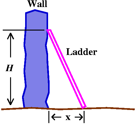 |
Such a problem is almost always in the Related Rates chapter of
calculus books, maybe about problem #7 or 8 of 20 problems: not
considered really difficult.
If H=the height of the top of the
ladder, and if x=the distance of the foot of the ladder to the base of
the wall, then H2+x2=132. When x=5,
then H=12 (wow, a textbook problem with a 5-12-13 right
triangle). Then d/dt the equation. The result is
2HH´+2xx´=0, so H´=-5/H. So the answer to the problem
posed is -5/12 ft per sec. The alert student will report that the
minus sign means that the ladder's top is moving down.
This is all nice, but I can make it weird. It becomes a workshop
problem (remember those) if I ask in addtion: what's the height of the
ladder when the velocity of the top of the ladder breaks the speed of
light? So let's see: 5/H should be (miles/sec·ft/mile)
186,000·5,280 etc. The height is about 5 times 10-7
feet (uhhhh ... 1500 angstroms? infrared light??). Ask your local
calculus teacher about this situation.
We will do more with the heat equation.
HOMEWORK
Read sections 13.1, 13.2, and 13.3 of the text.
Please hand in on Monday, November 28, the following problems:
13.1: 3, 15; 13.2: 1; 13.3: 1
Textbook problem presentations
People presented problems from section 12.3. I reminded students of
the review session Wednesday evening.
I view this part of the course as the payoff. I hope you will feel
that it is "worth the trip". Here I will show you certain well-known
and simple models of physical situations. The assumptions needed to
understand the models are not elaborate, and, most amazingly, the
predicted consequences seem intuitively correct and can even, in many
situations, be experimentally verified, with very good accuracy.
The 1-dimensional heat equation
This is probably the simplest model so it is an easy choice as the
first to be discussed. The heat equation is applicable to a very wide
variety of situations. The one-dimensional heat equation describes the
flow of heat through a homogeneous bar of constant cross-section, with
the "lateral" (long) sides insulated. It also can be used to describe
diffusion (put a sugar into water and see what happens), the migration
of moose in a narrow valley, or even the spread of gossip. What I did
was reproduce what is in the text on pages 692-693. Some students had
already seen such a discussion, but it may be new to others. I think
seeing the derivation is good, because the assumptions of the physical
model are fundamental to applying the whole theory. Even the names of
the various physical constants can be useful to know. There are many
similar sources available on the web. See, for example, this
web page. Another derivation is given on this page. and
yet another is here.
If you are someone who finds pictures very helpful (I certainly do),
you may find the various animations of solutions of the initial value
problem for the heat equation on
this web page useful.
 Suppose we have the heat equation
So after I went through the discussion, and tried to ask people if
steps of the derivation seemed sensible (for example, why a
minus sign relating the time derivative of heat to the space
derivative of temperature?) the usefulness of the equation may not be
apparent. We know ut=uxx where the subscripts
represent derivatives. Here u(x,t) is supposed to be the temperature
at time t at position x in a thin homogeneous bar whose lateral side
are kept insulated (no heat flow through the long side!). The bar is
supposed to overlay the interval [0,L]. Since this is a math course, I
have set all of the darn physical parameters equal to 1. The function
u(x,t)=3x2+5x+6t is a solution of the heat equation (how to
check this: two x derivatives give just 6, and one t derivative gives
6). But what the heck does this mean? Is this physically useful? Who
could care?
Some physical settings for the heat equation
Here are versions of the first problems usually considered with this
physical model.
- The setup Think of a bar with a certain distribution of
heat initially, and
that somehow one end of the bar (at x=0) is kept at temperature
u0 and the other end (at x=L) is kept at temperature
uL. For example, we want a house heated inside to some nice
warm temperature, while, in winter, the outside is rather chillier. A
thin tube of the barrier between the inside and the outside could be
modeled by our equation. Notice that the heating system of the house
wants to keep u(0,t)=u0 for all time, t, and the winter
forces u(L,t)=uL for all time, t.
The expected result We would guess that the initial temperature
distribution would likely not matter very much. The heat in the bar
will "evolve" as t-->infinity and tend towards a simple linear
interpolation between u0 and uL.
The math problem There is an initial temperature distribution,
u(x,0)=f(x) given for x between 0 and L (an initial
condition). Also required are u(0,t)=u0 and
u(L,t)=uL for all time. These are boundary
conditions. The phrase boundary value problem is applied to
all of these complicated specifications.
- The setup Think of a bar with a certain distribution of
heat initially, and that somehow both ends of the bar are insulated:
no flow of heat is possible in or out of the ends. Maybe a diffusion
setup is simpler to understand here. We sprinkle (?) sugar into a tube
of water, and no further additions or subtractions to the tube are
made. Then we try to study how the concentration of the sugar
evolves. Presumably there is Brownian motion (caused by "random"
ambient heat) which moves things around.
The expected result Over a long time (a long, long time ...) I
would expect the sugar to be close to uniformly distributed in
concentration. There's no reason for lots of suger (or too little
sugar) to be in any one chunk of the tube: this would be remarkably
unlikely. So the concentration of sugar, u(x,t), would be close to
constant as t-->infinity.
The math problem There is an initial {temperature|sugar
concentration} distribution,
u(x,0)=f(x) given for x between 0 and L (an initial
condition). Also required are that the {heat|sugar} doesn't flow
out. What math condition matches this? ux(0,t)=0 and
ux(L,t)=0 for all time. These are conditions on the
flux (a neat word to use instead of flow so that people
won't understand). This is another boundary value problem.
What we want is to solve these boundary value problems for the
heat equation and check that the solutions are as predicted. It is
truly remarkable that things will work out well: we'll see that
the model does predict this behavior. Wait 'til next time!
Phlogiston
Here's a link
to an old theory of heat. You may find it particularly interesting if
you have a good chemistry background. Enjoy!
HOMEWORK
Study for the exam.
Maintained by
greenfie@math.rutgers.edu and last modified 11/21/2005.