Math 421 diary, fall 2004, part 3:
Fourier Series
Thursday, November 11
The exam will cover up to and including section 12.3, as mentioned. So I asked for vigorous
volunteers to put the syllabus problems for 12.3 on the board. Things
actually went fairly well. I used fabulously interesting technology to
put student solutions on the board. And I tried to ask some
"interesting" questions. Below is an approximate record of what we
discussed.
Problem #
Student | Link to the student's solution; some further remarks |
|---|
12.3: 3
Mr. Klumb |
Here
is Mr. Klumb's witty response to the
question. He showed that the function was not odd and also was not
even by examining integrals of the function.
Another solution is the following: f(2)=22+2=6 and
f(-1)=(-1)2+(-1)=0. If f were odd, then f(-2) should be
-f(2) but it is not. If f were even, then f(-2) should be f(2) but it
is not. So f is neither odd nor even.
|
12.3: 5
Mr. Klami
| Here
Mr. Klami verifies that
e|x| is even. To check that a function is even or is
odd one must supply evidence that the necessary equations (f(-x)=f(x)
for f even, and f(-x)=-f(x) for x odd) are correct for all of the
implied values of x. Since, for example, the collection of x's is
frequently all positive x's, it isn't feasible to check these
computations by listing equations verifying agreement at each x. (I
can't write an infinite number of equations, anyway!) Therefore people
usually use algebra (in this case, relying on |x|=|-x|) or use
geometry (a sketch of e|x| which is symmetric with respect
to the y-axis. Mr. Klami actually provides both sorts of evidence.
|
12.3: 7
Mr. Novak
| Here
Mr. Novak checks that a function
is odd. Again, he supplies both graphical and algebraic evidence.
|
12.3: 13
Mr. Shah
| Here
is the first (in this set of
problems) computation of a Fourier series. In this case it is a
Fourier cosine series for x on the interval [0,Pi]: the even extension
of x is used. Here is a picture on [-Pi,Pi] of the function and its
partial sum up to the cos(3x) term.
|
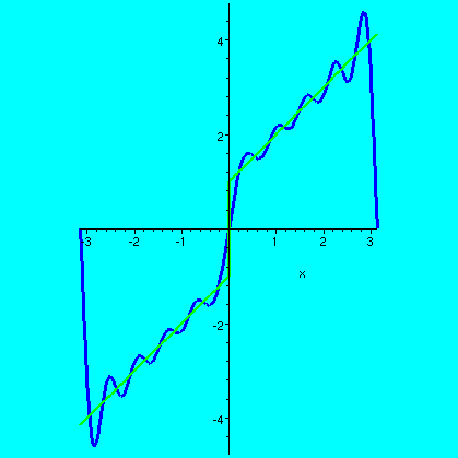
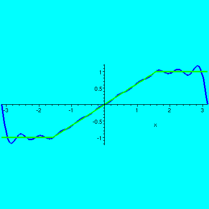
12.3: 19
Mr. Shaw
| Here
is an odd function on [-Pi,Pi]
and its corresponding Fourier series. Since the function is odd, all
of the cosine coefficients are 0, and the series is a sine series.
Here's a picture of the function and the partial sum of its sine
series up to sin(10x). I think the jump and overshoot behaviors are
apparent.
|
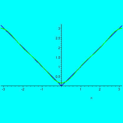
12.3: 23
Ms. Horn
| Here is a Fourier cosine series of an
even function, and below is a picture of the function and its
extension to [-Pi,Pi] together with the terms of its cosine series up
to cos(4x).
|
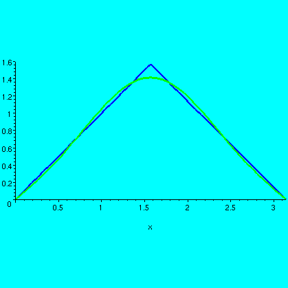
12.3: 29
Mr. Pierre-Louis
| Here are some elaborate computations
of Fourier sine and cosine expansions of the same function. What a lot
of work!
Here is a picture of the function analyzed by Mr. Pierre-Louis and (on
the left) the terms of the Fourier sine series up to sin(4x) and (on
the right) the terms of the Fourier sine series up to cos(4x).
Both the odd and even extensions of this function are continuous
everywhere, so there is no jump phenomenon. The corner does disappear
in the graphs of these partial sums, however.

|
12.3: 35
Mr. Sosa
| I'm sorry but I don't seem to have the student solution for
this problem.
Maple tells me that
the zeroth cosine coefficient is 4Pi2/3, and
the nth cosine coefficient is
        2   2
  4 (2 n  Pi  sin(Pi n) cos(Pi n) - sin(Pi n) cos(Pi n)

                           2           /      3
         + 2 Pi n cos(Pi n)  - Pi n)  /  (Pi n )
                                     /
and the nth sine coefficient is
         2   2          2    2   2            2
  4 (-2 n  Pi  cos(Pi n)  + n  Pi  + cos(Pi n)  - 1

                                         /      3
         + 2 Pi n sin(Pi n) cos(Pi n))  /  (Pi n )
                                       /
The n3's on the bottom occur because of two integrations by
parts.
 Here's a picture of the function and a partial sum of the Fourier
series up to sin(10x) and cos(10x). You can see the Gibbs phenomenon,
I hope, for the jump located at 0"="2Pi (the quotes are because I
don't really believe the numbers are equal, but Fourier series think
that these two numbers are the same.
Here's a picture of the function and a partial sum of the Fourier
series up to sin(10x) and cos(10x). You can see the Gibbs phenomenon,
I hope, for the jump located at 0"="2Pi (the quotes are because I
don't really believe the numbers are equal, but Fourier series think
that these two numbers are the same.
|
Parseval
The homework problems in 12.2 (such as #15) should have convinced you
that there are many weird equations which Fourier series can
verify. There's one that I should tell you about because it has
physical meaning and you should know it. It is called Parseval's
Theorem or Parseval's equation, or, maybe, just Parseval. Suppse f(x)
is a 2Pi periodic function. Then we know
f(x)=a0/2+SUMN=1infinity(ancos(nx)+bnsin(nx))
If you try to compute
 -PiPi(f(x))2dx and use the
equality, then interesting things occur. Because of orthogonality,
when we "expand" the sum and square it and then integrate, all of the
"cross terms" (say terms like sin(17x)cos(53x)) will integrate to
0. Also, because of the normalization coefficients, we get the
following
-PiPi(f(x))2dx and use the
equality, then interesting things occur. Because of orthogonality,
when we "expand" the sum and square it and then integrate, all of the
"cross terms" (say terms like sin(17x)cos(53x)) will integrate to
0. Also, because of the normalization coefficients, we get the
following
| Parseval's
Equation
-PiPif(x))2dx=a02/2+SUMn=1infinity(an2+bn2)
|
Again, in many applications,
-PiPi(f(x))2dx has a physical
meaning. For example, in many simple systems, this might be the energy
of a signal or a vibration. The an2's and
bn2's
could then be the amount of energy in various harmonics. In many
physical situations, a few low harmonics have most of the energy.
I will try to have extra office hours Wednesday
afternoon and early evening. Please
study for the exam. Also please begin
reading chapter 13.
I began the study of what the text calls Classical Equations and
Boundary-Value Problems. So we need a new diary!.
Tuesday, November 9
The exam on Thursday, November 18, will cover
what we've done on linear algebra
and introductory Fourier series (12.1-12.3).
|
|---|
|
|---|
|
|---|
| Vocabulary of the day |
|---|
|
acolyte
1. [Relig] a person assisting a priest in a service or procession.
2. an assistant; a beginner.
|
electrolyte
1. a substance which conducts electricity when molten or in
solution, esp. in an electric cell or battery.
2. a solution of this.
|
We had more fun with Fourier series. I reviewed the
formulas for Fourier coefficients. I wrote also how these were
used to assemble the Fourier series for a function. I noted that if a
function f were periodic with period 2Pi, then any interval of length
2Pi will be good for computing the Fourier coefficients. So, for
example, if I wanted a14, what I wrote last time is
(1/Pi)02Pif(x)cos(14x) dx and the
textbook has
(1/Pi)-PiPif(x)cos(14x) dx. But if for
some peculiar reason you wanted to use
(1/Pi)668668+2Pif(x)cos(14x) dx you
would get the same answer. Of course, for this, you should realize
that the function f(x) must be periodic with period equal to 2Pi.
Now what should we expect about the Fourier series of f(x)? I really
tried to think about the levels of information engineering students
should know about Fourier series.
Primary level
(What you really need to know)
On average, if you look at a "high" partial sum of the Fourier series
for f, then random samples of the values of this partial sum will be
close to the values of f(x). A precise statement is that the mean
square error will --> 0 as more terms are taken of the partial
sums.
Secondary level
(What you should know for Math 421)
The sum of whole Fourier series for a function, f, will be f(x) if f
is continuous at x. If f has a jump discontinuity at x, then the sum
of the whole Fourier series will be
(f(x-)+f(x+))/2, the average of the left and
right hand limits of f. Notice, though, that from the point of view of
Fourier series, 0 and 2Pi are the same, so the left side of 0 is the
left side of 2Pi, and the right side of 0 is the right side of
2Pi.
Comment This property really isn't just for 421, but may also
be useful in applications: I may be exaggerating about my
classifications!
Tertiary level
(What Fourier series enthusiasts might know)
The Gibbs phenomenon: if f has a jump discontinuity at x, then the
partial sums exhibit over and undershoots very near the jump, and the
bumps are opposite direction of the jump.
Notice, please that the sum of the whole Fourier series does
not does not have this behavior. Its behavior was described
above. I remarked that I did know of some real-world applications
where this Gibbs phenomenon was important, but I didn't know very
many.
Example 1
Suppose f(x)=5sin(x)-2cos(3x)+8cos(17x). What is the Fourier series
of f(x)? This is a very cute problem. The Fourier series of f(x) is
...5sin(x)-2cos(3x)+8cos(17x). It is its own Fourier series. Why is
that? Any other sine/cosine coefficient would be gotten by integrating
(the an or bn formulas). But the
other sine/cosine functions are all orthogonal to these. So, for
example, a17 is gotten by multiplying f(x) by cos(17x) and
integrating from -Pi to Pi. Hey: by orthogonality this is 0. What about
a17? Well, by orthogonality you only need to "worry" about
(1/Pi)-PiPi8(cos(17x))2dx, and (we
discussed this at great length!) this is just 8. The darn 1/Pi in the
original formula is included (orthonormalization!) to make the
coefficient come out correctly.
Then I went further. I asked people what
-PiPi (f(x))2dx was. Well, look at
[5sin(x)-2cos(3x)+8cos(17x)]2. "Expand" this square. Some
terms are 0 very rapidly (the "cross terms") because of
orthogonalization. What we have left is
-PiPi52(sin(x))2+(-2)2(cos(3x))2+82(cos(17x))2dx.
This is just Pi(52+22+82)=93Pi (I
hope, if I added correctly).
You certainly can do this computation by integrating everything in
sight. This would be a lot of work, and I think you might not compute
things correctly.
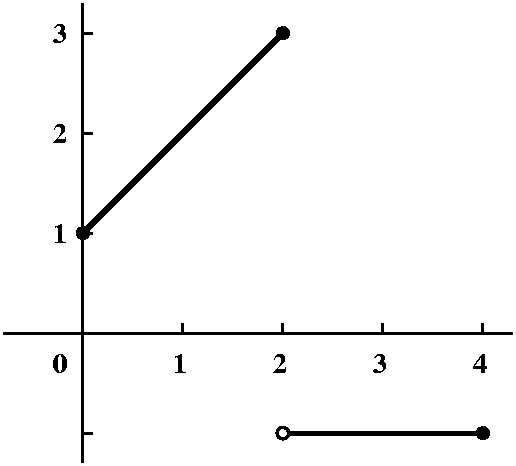
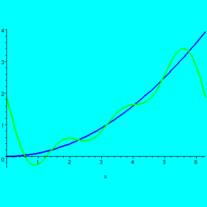
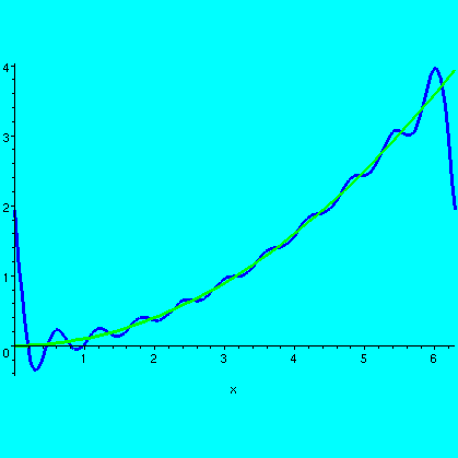
 Example 2
This example is more computationally intricate, especially when done
"by hand". f(x) is defined initially on the interval [0,Pi]. It is
piecewise linear, and is the sort of function we encountered in our
study of Laplace transform methods. The points (0,0) and (Pi/2,1) and
(Pi,1) are on the graph, which suggests that f(x) be (2/Pi)x in the
interval 0<x<Pi/2 and f(x)=1 for Pi/2<x<Pi. I asked for
the Fourier series of f(x). Objections were raised immediately,
because this function wasn't defined on [-Pi,Pi]. We decided to use
the extension suggested by Mr. Novak, mainly, just let f be 0 for
negative x's. Well, but remember this is only a recipe for -Pi to Pi,
and f(x) is extended periodically elsewhere.
I then actually computed, by hand (with a little help from the devil's
machine owned by Mr. Klumb, the
Fourier coefficients. This involved integrating by parts. I
hope that students can integrate by parts.
I just asked my friend (?) Maple to do the same
computation. The results were:
The cosine coefficients, a(n):

                                          Pi n
                   sin(Pi n) Pi n + 2 cos(----) - 2
                                           2
                   --------------------------------
                                    2
                                Pi n
The sine coefficients, b(n):

                                            Pi n
                    -cos(Pi n) Pi n + 2 sin(----)
                                             2
                    -----------------------------
                                    2
                                Pi n

a(0);

                                  3
                                 ---
                                  8
The n2's occur because of the integration by parts. I need
to evaluate a(0) separately, since I can't just plug in n=0 in a
formula with n in the bottom (yes, I could use L'Hopital's rule, but I
could also just evaluate the integral).
and just for the fun (?) of it, here is the partial sum up to third
order, of the Fourier series of the Novak extension of f(x):
        2 cos(x)   (Pi + 2) sin(x)   cos(2 x)       sin(2 x)
  3/8 - -------- + --------------- - -------- - 1/2 --------
            2              2             2             Pi
          Pi             Pi            Pi

               cos(3 x)       (3 Pi - 2) sin(3 x)
         - 2/9 -------- + 1/9 -------------------
                   2                    2
                 Pi                   Pi
|
And here is a picture of the Novak extension together with the
10th partial sum of its Fourier series. You can see that
the Fourier series is trying to get close to the Novak
extension. On mostg of the horizontal line segments and on the tilted
line, the partial sum of the Fourier series is wiggling above and
below, causing the visible alternation in colors (yes, I regret the
color choices, but I am too busy to try to fix them!). At the
endpoints, though, the partial sum wants to have the same value at
-Pi and Pi. So the value the partial sum takes is 1/2, the appropriate
average of 0 and 1. Also, the Gibbs phenomenon is visible, if you care
about it. |
|
Theory predicts the following:
| Graph of the Novak extension |
The sum of the whole Fourier series
of the Novak
extension of f |
|---|
 |
 |
The Fourier series thinks that the function is repeated periodically,
every 2Pi. So at x=Pi, the Fourier series sees 1 to the left and sees
0 to the right, and it says that its value should be 1/2, the average.
I remarked that if I changed the function's value at one point, say I
moved 0 to 78 at x=-.13, then the Fourier coefficients would not
change, because they depend on integrals, and integrals which
basically average, don't care about values at one point. And the
Fourier series would "heal" the whole in the graph, since at -.13, the
left and right limits are both 0, so the Fourier series would report
0.
The even extension
There are several standard ways of extending a function defined on
[0,Pi]. One is the even extension, which asks for a function so
that f(-x)=f(x). To get the graph, just flip what you are given across
the y-axis. There are some interesting consequences. One is that all
of the Fourier sine coefficients are 0. Why? Look at
bn=(1/Pi)-PiPiF(x)sin(nx)dx
When we change x to -x, the integrand, F(x)sin(nx) changes to
F(-x)sin(-nx) which is the same as -F(x)sin(nx). Since we're looking
at an interval balanced around 0 (from -Pi to Pi) the contribution at
x of F(x)sin(nx) is exactly balanced out by -F(x)sin(nx) at -x. So all
of the bn's are 0.
|
|
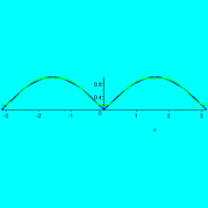
I had Maple compute the third
partial sum of the Fourier series for the even extension of f. Here it
is:
                    4 cos(x)   2 cos(2 x)       cos(3 x)
              3/4 - -------- - ---------- - 4/9 --------
                       Pi          Pi              Pi
You can see why this is called
the Fourier cosine series for f.
| I also had Maple graph the even extension and
some partial sums. The approximation is really good. On the left is
the even extension and just the first three terms (the constand and
cos(x) and cos(2x) terms): already quite close. The picture on the
right shows the even extension and the terms up to cos(10x). In this
picture, two distinct graphs can hardly be seen since they are so
close. Here the sum of the whole Fourier series will exactly be equal
to the function -- there are no jumps. |
|
The odd extension
Now with f defined on [0,Pi] we ask that f(-x)=-f(x). Flip the graph
over the y-axis, and then over the x-axis. Now because
an=(1/Pi)-PiPiF(x)cos(nx)dx
and
F(-x)cos(-nx)=-F(x)cos(nx) using the oddness of this extension, we see
that all of the an's are 0. Here's the beginning of this
Fourier series:
        2 (Pi + 2) sin(x)   sin(2 x)       (3 Pi - 2) sin(3 x)
        ----------------- - -------- + 2/9 -------------------
                 2             Pi                    2
               Pi                                  Pi
Not surprisingly this is called
the Fourier sine series for f.
| Here's a Maple graph of the odd extension of
f(x) together with the sum of the first 10 terms of the Fourier sine
series (up to and including the sin(10x) term). The series gets quite
close on the tilted line segment, and attempts to be near the two
horizontal segments. Of course, there is, in effect, a jump
discontinuity at -Pi and Pi. From the Fourier point of view, the odd
extension is repeated every 2Pi. So at, for example, x=Pi, the
function has a left limit of 1 and a right limit of -1, so the series
hops from 1 to -1. To me the Gibbs bumps are showing up.
|
|
Now what does theory predict here?
| Graph of the even extension |
The sum of the whole Fourier series
of the even
extension of f |
|---|
 |
 |
The sum of the Fourier sine series of f (that is, the Fourier series
of the odd extension of f) is equal to the original function except at
the ends, where it averages the left and right behavior.
Volunteers
The syllabus for the course contains the
following entry:
| 12.3 |
Fourier Sine and Cosine Series |
3, 5, 7, 13, 19, 23, 29, 35 |
Since the exam will cover this section, I requested volunteers to do
the problems in claas on Thursday. The following students either
couldn't evade my attention, or, rarely, actually volunteered to put a
problem on the board at the beginning of class Thursday. I thank
them for their efforts in advance. Mr. Lin could not volunteer since he was
in Texas. After class, he mysteriously precipitated (chem engineers do
that).
| Problem # | Student |
|---|
| 12.3: 3
| Mr. Klumb
|
| 12.3: 5
| Mr. Klami
|
| 12.3: 7
| Mr. Novak
|
| 12.3: 13
| Mr. Shah
|
| 12.3: 19
| Mr. Shaw
|
| 12.3: 23
| Ms. Horn
|
| 12.3: 29
| Mr. Pierre-Louis
|
| 12.3: 35
| Mr. Sosa
|
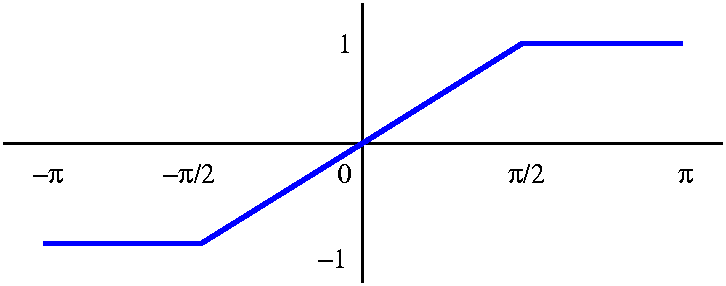
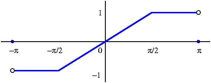
QotD I quickly sketched something on the board, and asked
people to sketch the even and odd extensions of it.
| Original random function's graph |
Even extension | Odd extension |
|---|
 |
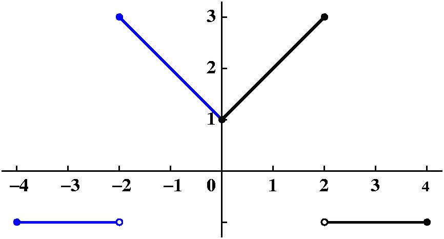
|
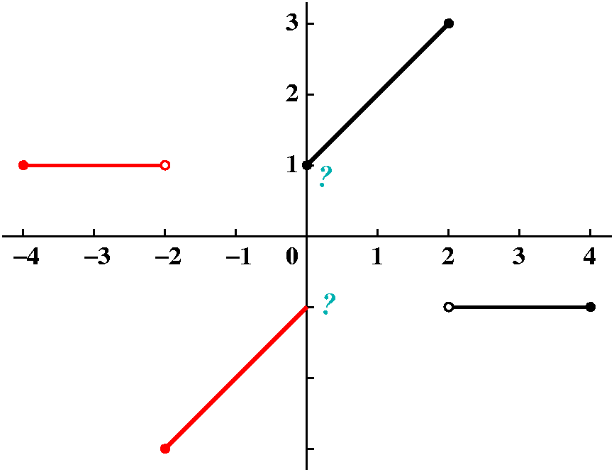 |
Complaint Department
Ms. Tozour complained that the qotd was
not "well-posed"(badly stated question). She stated (see the ?'s in the third graph) that the
value(s?) of the odd extension at 0 was not clear. I agree with her.
Thursday, November 4
Alice Cooper?
Although a real professional photographer was there, together with his
faithful assistant, I hope you did not expect a personage like Alice
Cooper. Oh well, we just lost about 1/2 hour of instructional time and
lots of concentration. I am sorry. Back to work.
Orthogonality
This is in the text, but following what we did last time, you should
know:
- 02Pisin(nx)sin(mx)dx=0 when n and m
are different integers.
- 02Picos(nx)cos(mx)dx=0 when n and m
are different integers.
- 02Pisin(nx)cos(mx)dx=0 when n and m
are integers.
Therefore the collection of functions {sin(nx),cos(nx)} (for n an
integer) forms an orthogonal family of functions using our new notion
of inner product. Notice that when n=0 there are two almost silly
special cases: sin(0x) is the constant zero function, and
cos(0x) is the constant 1 function.
To continue the analogy I started last time, I need to orthonormalize
these functions. Since sin2+cos2=1, and the
wiggles are the same over an interval of length 2Pi, I know that
02Pisin(nx)2+cos(nx)2dx=2Pi
and each of 02Pisin(nx)2dx and
02Picos(nx)2dx are the same, so
if n is an integer >0,
02Pisin(nx)2dx=Pi and
02Picos(nx)2dx=Pi.
Of course, for the silly case (n=0),
02Picos(0x)2dx=2Pi. (We
don't care about the 0 function, so from now on I'll drop any mention
of stuff corresponding to sin(nx) when n=0.)
The Fourier series of a function
If F(x) is a function defined on the interval [0,2Pi], define
an=(1/Pi)02PiF(x)cos(nx)dx
bn=(1/Pi)02PiF(x)sin(nx)dx
The Fourier series of F(x) is the infinite series of functions
a0/2+SUMN=1infinity(ancos(nx)+bnsin(nx))
where
an=(1/Pi)02PiF(x)cos(nx) dx
for n integer, n>=0
bn=(1/Pi)02PiF(x)sin(nx) dx
for n integer, n>0
Weird things to note
Well, these are weird but they are what's usual in the subject. Notice
that the a0 term is divided by 2. That's because the
normality constant for cos(0x) is 2Pi, not Pi. And also notice
that the rest of the normalizing constants come off the formulas for
the coefficients. In many standard linear algebra contexts, the darn
formulas have the normalizations (those silly square roots) somehow in
both the vectors and the coefficients of the vectors. Maybe what is
done with Fourier series is more sensible.
You tell me how the Fourier series of a
function relates to the function
I gave the class a handout. I
wanted, in observation and discussion with students, to
discover relationships (some subtle) between a function and its
Fourier series (or, rather, since one can't add up all of any
real infinite sum, the partial sums of the Fourier series): more
heuristic stuff.
I would also like to have the Maple commands shown there
available for you to copy, if you have the time and desire to
experiment with them. Here they are:
- g:=n->(1/Pi)*int(F(x)*sin(n*x),x=0..2*Pi); Creates the sine
coefficients.
- h:=n->(1/Pi)*int(F(x)*cos(n*x),x=0..2*Pi); Creates the cosine
coefficients.
- Q:=N->h(0)/2+sum(h(n)*cos(n*x)+g(n)*sin(n*x),n=1..N); Adds
things up and provides a linear combination of trig functions which is
the Nth partial sum of the Fourier series of F.
- plot({F(x),Q(3)},x=0..2*Pi,thickness=3,scaling=constrained);
Plots the function F(x) together with the third partial sum of its
Fourier series.
Before any of these instructions are executed, a definition of F(x) is
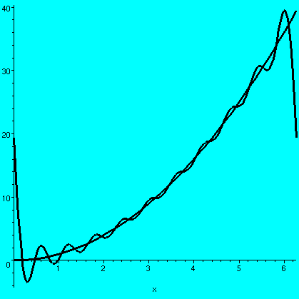
useful. The first function I investigated is (1/10)x2,
which is defined by the command:
F:=x->(1/10)*x^2;
After this definition I checked to see if things were "working" by
requesting Q(3):
>Q(3);
            2
        2 Pi
        ----- + 2/5 cos(x) - 2/5 Pi sin(x) + 1/10 cos(2 x)
         15

                - 1/5 Pi sin(2 x) + 2/45 cos(3 x) - 2/15 Pi sin(3 x)
Each coefficient is gotten by integrating by parts (the QotD
was to find an antiderivative of x2cos(x) without
electronic help: this is two uses of integration by parts).
This F(x) and the 3rd partial
sum of its Fourier
series |
This F(x) and the 10th partial
sum of its Fourier
series |
This F(x) and the 20th partial
sum of its Fourier
series |
 |
 |
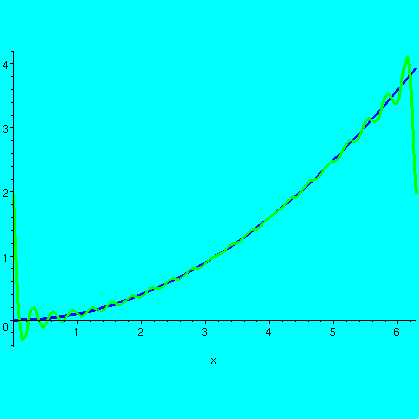 |
The graphs of the Q(n)'s (the partial sums) get closer to the
graph of F(x) as n increases.
What does closer mean? This turns out to be a rather difficult
question, both theoretically and in practice.
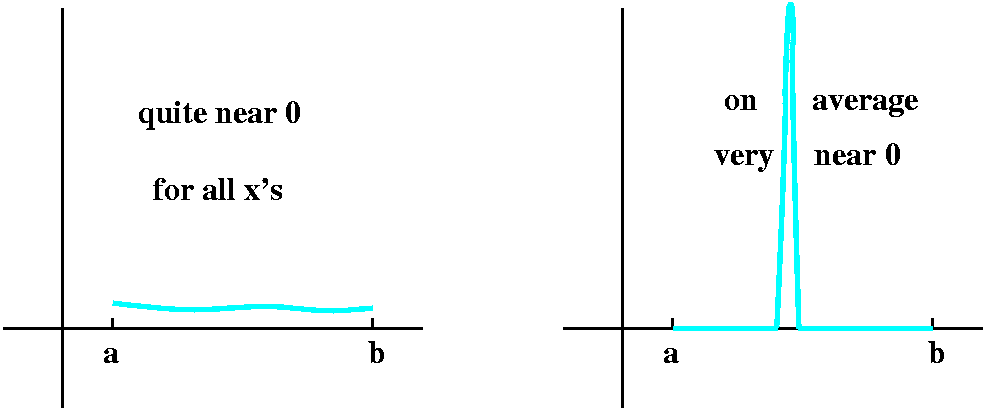
The pictures should show some of the difficulty. For example, you may
want a function to be small on [a.b]. A very strict
interpretation might be to have the values, f(x), very close to 0 for
all x. But suppose you were really modelling some process which you
expected to sample, somehow "randomly", on the interval, a few times
(10 or 100 or ...). Maybe you would be happy enough controlling the
average distance to 0. So things are complicated.
In the pictures of our function F(x) and various partial sums,
inside the interval the partial sums are getting close to the
values of the function. At the end points (0 and 2Pi) they aren't
getting close ... what the heck. Also, if you look really closely at
the graphs, you can see tiny bumps near the "ends" which represent
some complicated phenomena. Well, one thing at a time.
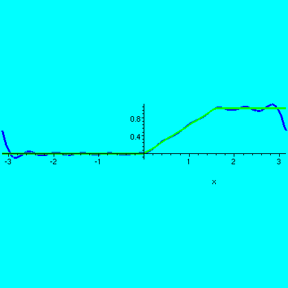
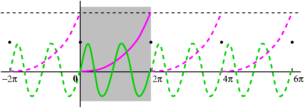
What the Fourier series sees...
We get the Fourier coefficients by integrating the product of a sine
or cosine on [0,2Pi] (the solid green curve) by our function F(x) (the
solid magenta [?]) curve). One point of view is that everything goes
on inside the shaded box. But the trig function goes on forever, and it
is periodic with period 2Pi. To the trig function, our F(x) might as
well be "extended" with period 2Pi to the left and to the right
forever. Notice that the trig function will try at, say, 0, to
approximate the values from both the left and right of the extended
F(x). This extended F(x) has a jump discontinuity at 0, and the trig
function, in trying its approximation, settles on being halfway
between the ends of the jump. This is the collection of black dots in
the picture at half the height of F(x) at x=2Pi.
The partial sums of the Fourier series try very hard to get close to
F(x). If F is continuous at x, then they will converge to F(x). If F
has a jump discontinuity at x, then they will converge to the average
(really!) of the left and right hand limits of F at x (the middle of
the jump).
Gibbs: the overshoot
J.
Willard Gibbs received the first U.S. doctorate in engineering in
1863. He saw that at a jump discontinuity, there is always an
overshoot of about 9% in the Fourier series. On the top side, the
overshoot is above, and on the bottom side, below. These bumps get
narrower and closer to the jump, but they never disappear!
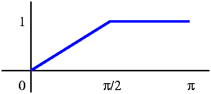
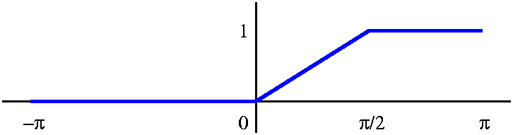
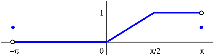
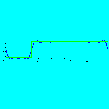
My next example was U(x-{Pi/2}), the Heaviside step or jump at
Pi/2. This function is 0 to the left of Pi/2 and is 1 to the right of
Pi/2. In Maple, the following formula describes the function:
F:=x->piecewise(x<Pi/2,0,1);
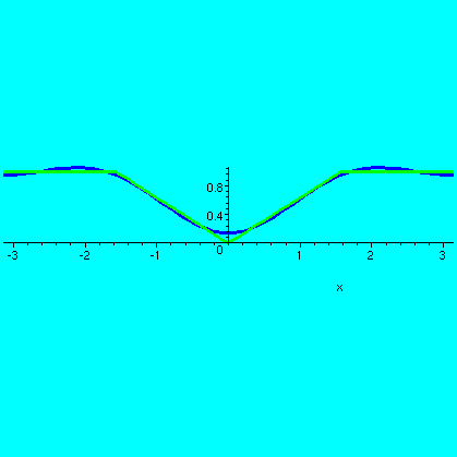
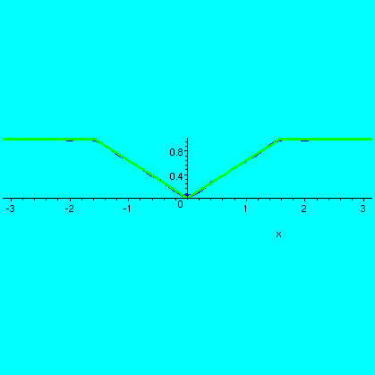
Here are the pictures for this function.
This F(x) and the 3rd partial
sum of its Fourier
series |
This F(x) and the 10th partial
sum of its Fourier
series |
This F(x) and the 20th partial
sum of its Fourier
series |
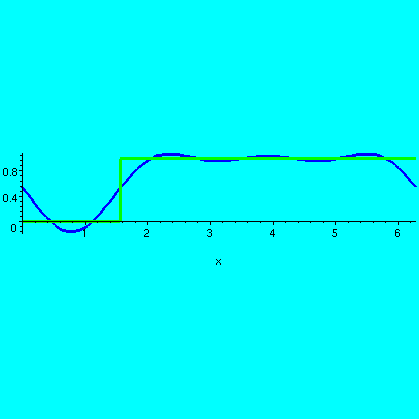 |
 |
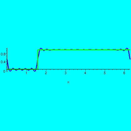 |
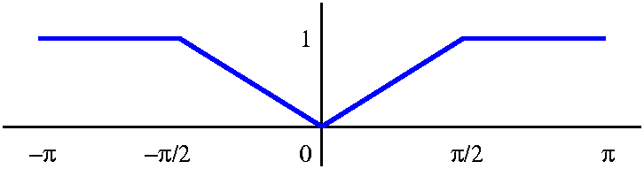
I hope you see that the partial sums detect two jump discontinuities,
one at Pi/2, certainly, but another one at 0=2Pi (well, they are the
same numbers to sine and cosine) as well!
HOMEWORK due Tuesday,
November 9.
Read sections 12.1, 12.2, and 12.3 of the text. Hand in:
12.1: 7, 15
12.2: 1, 5, 9, 15, 17
Tuesday, November 2
#1
The next exam will be given during the regular class period on
Thursday, November 18, 2004.
Please begin to read sections 12.1, 12.2, and 12.3 of the text.
#2
Why I wouldn't want to be an engineer
This is an advisory note to both chemical and mechanical
engineers. When mistakes are made, the results can be serious. When an
academic mathematician makes a mistake, the grade can be computed
again. Here are links to newspaper articles about the breaking of a 460,000 gallon tank full
of 50% sodium hydroxide solution this past weekend in nearby
New Jersey. Maybe there is no routine engineering, just routine
engineers!
The New York Times
The
Home News Tribune
I think a study of this incident would probably be an excellent senior
project!
#3
I want to begin the next part of the course. I attempted to
convince students that Fourier series would be an extended metaphor
(is this good or bad educationally?), analogous to the material we
just covered about symmetric matrices.So we looked at the symmetric
matrix C=
( 0 -1 1)
(-1  1 2)
( 1  2 1)
and found its eigenvalues and eigenvectors:
If  =1, v1=(2,-1,1)
If =-2, v2=(-1,-1,1)
If =3, v13=(0,1,1)
We noted that these were orthogonal, and then normalized
(divided by their length) to make them orthonormal. I will call
wj the vectors vj/||vj|| .The fact
that the
dot product of wi and wj is 1 if i=j and 0
otherwises leads one to observe that the matrix P=
( 2/sqrt(6) -1/sqrt(3)    0     )
(-1/sqrt(6)  1/sqrt(3) 1/sqrt(2))
(-1/sqrt(6)  1/sqrt(3) 1/sqrt(2))
has the interesting property
that the transpose of P will be the inverse of P.
Of course, PtCP is the matrix D=
(6 0 0)
(0 3 0)
(0 0 2)
and this is useful if you wanted to compute
C7 or eCt (which will help to solve a system of
ODE's with C as its coefficient matrix).
Then I asked the following weird question, which has a
wonderful answer. If I take a "random" vector in R3
then it is possible to write the vector as a linear combination of the
wj's (j=1,2,3). So if Q=(11,33,-7), then
Q=(some #1)w1+(some #2)w2+(some #3)w3
In general it might be irritating (possible, but irritating) to find
the coeffients. Here it turns out the computation is rather easy.
If Q=(some #1)w1+(some
#2)w2+(some #3)w3 then
take the dot product of Q with w1, say. The dot product
distributes over the linear combination. Yes, you should know what
this all means after 4 weeks of linear algebra and lots and lots of
vector manipulation in a bunch of different courses:
Q·w1=((some #1)w1+(some
#2)w2+(some #3)w3)·w1. If you distribute
the dot product, two terms become 0 and one term is just 1. So
Q·w1=(some #1. In our specific
case, with Q=(11,33,-7) and
w1=(2/sqrt(6),-1/sqrt(6),-1/sqrt(6)) the dot product is
exactly (22-33-1(-7))/sqrt(6)=-4/sqrt(6).
Many computer systems are optimized to take dot products, so this is
really useful.
Now the analogy
Things will get complicated here. For the remainder of this course,
the object is to study certain "classical" (a century old) ways of
getting solutions to the partial differential equations which are
supposed to model things like heat transfer or diffusion (the same
equation: H(x,t) is a function of 1-dimensional position) or string vibration (double derivative in t is the double
derivative in x: X(x,t) is the height at position x at time t of a
vibrating string) or plate vibration (double derivative in t is the sum
of the double derivative in both x and y where the deflection is a
function of position [x and y] and time, t).
It turns out that these partial differential operators are all
linear, and analyzing there solution can be accomplished by looking
for eigenvectors. In all cases, one needs functions whose second
derivative is a multiple of the original function (so the "eigen"
characterization will be valid). So we throw out such things as
x. For the most part, we also won't consider, say,
e47t, because this function gets big as you differentiate
it.
Historically the functions which Mr. Fourier used were sin(nx) and
cos(nx) where n is an integer. These functions will turn out to be
eigenfunctions for essentailly all of the partial differential
equations we will consider.
The vectors in our setup will be functions. The dot
product we will use will be the following: if f and g are
functions on the interval [a,b], then the "dot product" will be
abf(x)g(x) dx. You may well object that
this is too weird. Well, at least algebraically this behaves like the
inner product of vectors in Rn
(f·g=g·f and f·(g1+g2)=f·g1+f·g2
etc.).
What might be a bit more useful is to tell you the distance
between f and g which this inner product defines: this distance is
(abf(x)-g(x) dx)1/2. This is just about the same as the
root mean square error between f and g (usually people might want to
divide by b-a). This quantity should measure the average error
between the functions f and g. If it is small, then, on average, the
graphs of the functions f and g should be close.
Then just as in the Rn case we will try to write a function
f(x) as a sum, a very big sum:
SUMn=0infinity(coefficients)sin(nx)+(other coefficients)cos(nx).
This sort of sum is called a Fourier series.
Caution: the problem with convergence
I believe that the principle object of this course is to teach
engineering students methods which they can use to model and predict
practical problems. What I've just written is a real difficulty, a
conflict between my own "trade", and the course objective. I know that
the free and unrestricted use of infinite series almost inevitably
leads to problems and sometimes even errors. I will show you a very
simple example below. I remark that I will try to keep from stating
false results in this course, and try to help students from making
mistakes related to convergnece. But all I can do is caution you that,
generally, if you "push" known methods to handle new or unusual
situations, you may run into problems with convergence, and you may
make errors. This has happened repeatedly historically.
The simple example
For various reasons in such applications as probability, one may take
a matrix and compute its row sums and its column sums:
           Row sums
   (horizontal sums of the entries)
( 3 -7  8)    4
(10  2 11)   23
(-5  6 -8)   -7
  8  1 11
Column sums
(vertical sums of the entries)
and then the sum of the row sums
could be computed and also the sum of the column sums:
  4
 23
 -7
---
 20 column sum of the row sums

 8  1 11 | 20 row sum of the column sums
You will notice that the row sum of the column sums is the same as the
column sum of the row sums: easy, easy, easy.
It seems always true
that "the row sum of the column sums is the same as the
column sum of the row sums."
Now please think of an doubly infinite matrix. This will be a matrix
which has entries aij for all i and j positive integers. I
want you to consider one specific matrix. I will show you a small
piece of this matrix: FOREVER ------>
F( 1 -1 0 0 0 0 0 0 .....
O( 0 1 -1 0 0 0 0 0 .....
R( 0 0 1 -1 0 0 0 0 .....
E( 0 0 0 1 -1 0 0 0 .....
V( 0 0 0 0 1 -1 0 0 .....
E( 0 0 0 0 0 1 -1 0 .....
R( 0 0 0 0 0 0 1 -1 .....
|( 0 0 0 0 0 0 0 1 .....
|( . . . . . . . . ......
V
Let me try to be clear about this
(I wasn't too successful in class!). The matrix goes on to the right
and down forever. It is a banded matrix, 0 a few spaces
to either side of the main diagonal. The row sums are all 0, so the
column sum of the row sums is 0. What about the column sums? The first
one is 1, and all the others are 0. So the row sum of the column sums
is 1. And, unless you want 0 and 1 to coincide
0 and 1 are not equal
then you should see that interchanging infinite sums can get you into
trouble. This is only one example, and, unfortunately, bad things can
happen if we aren't a bit careful with some of the computations we
will do.
I will attempt to be careful, but, again, "problems and sometimes even
errors" are possible.
I then restated
|
Euler tells me ...
|
|---|
| eit=cos(t)+i sin(t) and
cos(t)=[eit+e-it]/2
and
sin(t)=[eit-e-it]/(2i)
|
|---|
and used this to compute
02Pisin(17x)cos(5x) dx. There are several
ways to do this integral. You can integrate by parts (you must do this
twice, and be somewhat careful). You can use certain trig identities
(this is the way the textbook does it). Or you can use Euler:
sin(17x)=[e17ix-e-17ix]/(2i) and
cos(5x)=[e5ix+e-5ix]/2 so that
sin(17x)cos(5x)=(1/4i)(e22ix-e-12ix+e12ix-e-22ix.
This may seem involved, but all I'm doing is manipulating exponents in
a standard fashion.
Easy integrals?
Suppose A is a non-zero integer. Then
02PieiAxdx={1/iA}eiAx]02Pi.
Now if x=0, eiA·0=1. If x=2Pi,
eiAx=eiA(2Pi)=cos(2Pi A)+i sin(2Pi A).
The cosine term is 1 (cosine at an even multiple of Pi is 1) and the
sine term is 0 (sine at any multiple of Pi is 0). Therefore the
integral is 0.
Now use this result with A=22 and A=-12 and A=12 and A=-22 to see that
02Pisin(17x)cos(5x) dx=0. The functions
sin(17x) and cos(5x) are orthogonal.
The QotD was to compute
02Pisin(7x)cos(7x) dx. I suggested using
the same (complex) methods. Mr. Pierre-Louis instead successfully used a
trig identity.
HOMEWORK
The next exam will be given during the regular class period on
Thursday, November 18, 2004.
Please begin to read sections 12.1, 12.2, and 12.3 of the text.
Maintained by
greenfie@math.rutgers.edu and last modified 11/2/2004.