March 30
Example 1
Let's take A=(2 1) (3 4)We saw in the last lecture that this A has two eigenvalues and we computed corresponding eigenvectors. Here they are:
For the eigenvalue
For the eigenvalue
I then created the matrix C=
( 1 1) (-1 3)and did some computations which I said I would explain afterwards. First, I created C-1.
( 1 1 | 1 0)~(1 1 | 1 0)~(1 0 | 3/4 -1/4) (-1 3 | 0 1) (0 4 | 1 1) (0 1 | 1/4 1/4)So C-1 is
(3/4 -1/4) (1/4 1/4)and you can check this easily by multiplying C-1 with C, and the result with be I2, the 2 by 2 identity matrix. I2 is
(1 0) (0 1)Now I computed the rather interesting product C-1AC. Since matrix multiplication is associative the way I group the factors doesn't matter. That is, C-1(AC) and (C-1A)C will give the same result. Now AC is
(2 1)( 1 1)=( 1 5) (3 4)(-1 3) (-1 15)and then C-1(AC) is
(3/4 -1/4)( 1 5)=(1 0) (1/4 1/4)(-1 15) (0 5)Maybe it is remarkable that the result turns out to be a rather simple diagonal matrix, D. On the other hand, let me try to explain what I'm doing.
Suppose I take a vector (x,y) in R2 and I try to investigate what multiplying the corresponding column vector by the 2 by 2 matrix C-1AC "does". The corresponding column vector is
(x)=x(1)+y(0)=a e1+b e2 (y) (0) (1)and multiplication by C distributes over this linear combination. So we just need to understand C e1 and C 1. I "build" C so that the results of these computations are eigenvectors of A corresponding to the eigenvalues
( 1) and (1) (-1) (3)Therefore when we multiply
x( 1)+y(1) (-1) (3)by A the result must be
x1( 1)+y5(1) (-1) (3)C changes bases from the "standard basis" of R2 to a basis of the two eigenvectors (I know it is a basis because the two vectors are linearly independent because the matrix C has an inverse!). What does C-1 then do? It changes back from the basis of eigenvectors to the standard basis. The important thing to observe is that x and y are just going to get changed to 1x and 5y, because we used the eigenvectors when we multiplied by A. So the result D, the diagonal matrix with entries 1 and 5, as the value of C-1AC therefore shouldn't be a surprise.
Comment Although C-1AC should be diagonal, I should confess when I'm doing these computations by hand (and even sometimes with the help of computers!) I make mistakes. And I confidently (!) expect the result to be diagonal, and it is not because, well, I may have "dropped" a minus sign, or I may have entered a command wrong in Maple or ... many, many reasons. There are lots of ways to be human, and "To err is human."
Another short digression
Another matrix we analyzed last time was
(1 283) (0 1)We learned that the only eigenvalue was 1 and that all eigenvectors are non-zero multiples of one vector: (1,0). Can this matrix be diagonalized as I just computed above? The answer is an emphatic No! An n by n matrix can be diagonalized exactly when there ia a basis of n eigenvectors of Rn, because those are the vectors which would supply us with a matrix, C, which changes coordinates. Sometimes reasons that a matrix can't be diagonalized are subtle and difficult to explain, but here it is evident: there aren't enough eigenvectors.
So now I diagonalized the matrix A=
(2 1) (3 4)Why should I/we care about this? There certainly turn out to be theoretical reasons, but there are many practical numerical reasons also. For example, I could want to compute powers of A. What's A6, for example? {Why you might want to compute high powers of matrices: it turns out that the "evolution" of certain systems under time is equivalent to looking at powers of matrices. We don't have enough time in the course to explain this.) Anyway, Maple told me that A6 is
( 3907 3906) (11718 11719)But I am worried. The matrix looks too nice, and maybe the answer is wrong or ... somehow something gout fouled up. Let me show you how to do some cheap and easy checking of this result.
We know that C-1AC=D. Therefore we could multiply on the left by C and on the right by C-1. The result would be A=CDC-1. Notice, please, that I must be very careful about the order, because matrix multiplication is not necessarily commutative. That is, order may matter, but "grouping" (associativity) does not. So we must be careful.
Since A=CDC-1 we can write
and we can regroup (associate, but not reorder!)
Now each product CC-1 becomes I2 and I2 is a multiplicative identity -- you can multiply by it and not change anything. Therefore
We can choose to compute A6 by computing D6 instead, and then pre- and post-multiplying by the appropriate matrices. Multiplying diagonal matrices is quite easy:
(k1 0 )(m1 0 )=(k1m1 0 ) ( 0 k2)( 0 m2) ( 0 k2m2)Therefore if
D=(1 0) then D6=(16 0 )=(1 0 ) (0 5) (0 56) (0 56)and I will not "simplify" further since I don't know offhand what 56 is. I can sort of compute CD6C-1, though. Let's see: D6C-1 is
(1 0 )(3/4 -1/4)=( 3/4 -1/4) (0 56)(1/4 1/4) (56/4 56/4)and now let's left multiply by C:
( 1 1)( 3/4 -1/4)=( [3+56]/4 [-1+56]/4) (-1 3)(56/4 56/4) ([-3+3·56]/4 [1+3·56]/4)What a mess this is! This mess can explain easily some of the (supposedly) correct answer, that A6 is
( 3907 3906) (11718 11719)Look: the entries in the top row in both answers do differ by 1, as do the entries in the bottom row. The "/4" is exactly what is needed to make things match up.
So A100 similarly could be computed by evaluating CD100C-1. Maybe this isn't too darn impressive to you but it is to me. Computing the 100th power of a 2 by 2 matrix directly is ... uhhh ... lots of computation. If, in real life we had a 36 by 36 matrix (that is really not too big) and I wanted to compute powers of this matrix efficiently, I certainly would prepare by diagonalizing it, computing C and C-1 and D. This would be much less work than a direct computation.
Matrix exponentials
I thought that this topic had been covered in 244. I'll go over this
quickly. Suppose Y(t) is a 2 by 2 matrix of functions of t, and Y(t)
is supposed to satisfy this differential equation: Y'(t)=AY(t). Just
as in scalar equations (this is 4 scalar equations, though!) we
should try to write Y(t)=KeAt where K is a constant matrix,
and At is the result of multiplying the entries of the matrix A by the
scalar t. How can we compute eAt? Let me show
you. This exponential is the sum, as n runs from 0 to infinity, of
(At)n/n!. But this is
C(Dt)nC-1/n!. And the entries of
(Dt)n/n! are
(tn/n! 0 ) ( 0 (5t)n/n!)If you sum this up from n=0 to infinity, the entries in the matrix are
(et 0 ) ( 0 e5t)and therefore eAt is exactly
C(et 0)C-1=((3/4)et+(1/4)e5t -(1/4)et+(1/4)e5t) ( 0 e5t) (-(3/4)et+(1/4)e5t (1/4)et+(3/4)e5t)The general idea is that all the work can be done componentwise on D, and, once A is diagonalized, you don't really need to do much with A itself. I also admit that the last computation was done by Maple, which has, for these things, much more patience than I do!
Example 2
Mr. Hunt kindly answered the QotD given last time. That was: find the eigenvalues of(0 2 1) (2 0 1) (1 1 1)He computed the characteristic polynomial, det(A-
I then asked the class to produce eigenvectors for each
eigenvalue. After some waiting, we discovered that you could almost
guess the eigenvectors,
since this is an in-class example. So:
When ![]() =0, we need (x1,x2,x3) so that
=0, we need (x1,x2,x3) so that
A-0I3=(0 2 1)(x1)=(0x1)
(2 0 1)(x2) (0x2)
(1 1 1)(x3) (0x3)We can guess the
answer(s)! It isn't too hard, since we know this is an in-class
example. The corresponding eigenvector is (all non-zero multiples of)
(1,1,-2).When
A-(-2)I3=(2 2 1)(x1)=(0x1)
(2 2 1)(x2) (0x2)
(1 1 3)(x3) (0x3)Again we guessed the
answer(s)! The corresponding eigenvector doesn't involve x3
at all, and it is (all non-zero multiples of)
(1,-1,0).When
A-3I3=(-3 2 1)(x1)=(0x1)
( 2 -3 1)(x2) (0x2)
( 1 1 -2)(x3) (0x3)This was somehow the
most difficult one to guess. Of course, we could do row reduction,
etc. Oh well. We can guess the
answer(s)! The corresponding eigenvector is (all non-zero multiples of)
(1,1,1).
The eigenvectors for this matrix are therefore (1,1,-2) and (1,-1,0)
and (1,1,1) corresponding to ![]() =0 and
=0 and ![]() =-2 and
=-2 and ![]() =3, respectively. I
could now diagonalize, etc. But I asked something more difficult of
the class. I remarked that this A was not "random", since it was
symmetric: A=At (a is its own transpose). I believe that
Mr. Ivanov first noticed that the
these eigenvectors were orthogonal. The dot product of two
different eigenvectors was 0. (That certainly did not happen with our
first 2 by 2 example.
=3, respectively. I
could now diagonalize, etc. But I asked something more difficult of
the class. I remarked that this A was not "random", since it was
symmetric: A=At (a is its own transpose). I believe that
Mr. Ivanov first noticed that the
these eigenvectors were orthogonal. The dot product of two
different eigenvectors was 0. (That certainly did not happen with our
first 2 by 2 example.
This is generally true. Please see pp.359-360 of the text for the
following results (which are not hard to verify). The results are
very useful in practice:
|
If A is a symmetric matrix, then the eigenvalues of A are all real and eigenvectors of distinct eigenvalues are always orthogonal.
There is always a basis of eigenvectors, so |
( 1 1 1) ( 1 -1 1) (-2 0 1)What if I were to take the transpose of this matrix:
(1 1 -2) (1 -1 0) (1 1 1)Now check this: the product of the second matrix with the first is
(6 0 0) (0 2 0) (0 0 3)so if I "adjusted" the lengths by multiplying the columns of the initial guess by constants, then the transpose would be the inverse. So I really should take C to be:
( 1/sqrt(6) 1/sqrt(2) 1/sqrt(3)) ( 1/sqrt(6) -1/sqrt(2) 1/sqrt(3)) (-2/sqrt(6) 0 1/sqrt(3))and then C-1 would be Ct:
(1/sqrt(6) 1/sqrt(6) -2/sqrt(6)) (1/sqrt(2) -1/sqrt(2) 0 ) (1/sqrt(3) 1/sqrt(3) 1/sqrt(3))This is wonderful -- well, wonderful because it is less work. Here is the general recipe:
|
If A is a symmetric n by n matrix, then take n orthogonal eigenvectors
(guaranteed by the previous fact) and normalize them: divide
each vector by its length so you get a multiple of the original
eigenvector which has unit length. Then assemble the vectors as column vectors to get a matrix C. The matrix C is orthogonal: C-1=Ct. Therefore CtAC=D, a diagonal matrix of the eigenvalues of A. |
Here A=
(0 2 1) (2 0 1) (1 1 1)which has eigenvalues 0 and -2 and 3. C is the matrix
( 1/sqrt(6) 1/sqrt(2) 1/sqrt(3)) ( 1/sqrt(6) -1/sqrt(2) 1/sqrt(3)) (-2/sqrt(6) 0 1/sqrt(3))and then I claim that CtAC is actually the diagonal matrix
(0 0 0) (0 -2 0) (0 0 3)If you are too tired to check this, well, I don't really blame you. Here is Maple's verification:
> eval(A);
[0 2 1]
[ ]
[2 0 1]
[ ]
[1 1 1]
> eval(C);
[ 1/2 1/2 1/2]
[ 1/6 6 1/2 2 1/3 3 ]
[ ]
[ 1/2 1/2 1/2]
[ 1/6 6 - 1/2 2 1/3 3 ]
[ ]
[ 1/2 1/2]
[- 1/3 6 0 1/3 3 ]
> evalm(transpose(C)&*A&*C);
[0 0 0]
[ ]
[0 -2 0]
[ ]
[0 0 3]
The first two instructions ask Maple to display the
data structures associated with A and C: they are our A and
C. The last instruction asks Maple to evaluate the matrix
product CtAC, and we get the predicted diagonal matrix of
eigenvalues. That's all for now.
The QotD was: suppose A is a 2 by 2 matrix and At=5A. What can you say about A and why is what you declare true?
Mr. Ivanov asked several times how "often" a matrix is diagonalizable. I tried to evade a general answer. For example, if the matrix is symmetric, then what I wrote above asserts it is diagonalizable. But the general question has been quite well-studied. An "average" (??) matrix should be diagonalizable, but you may have to allow for complex entries. One place to get the full story is Math 350, or look at any advanced linear algebra book.
March 25
A=(1 a) and B=(b) (0 1) (c)then AX=B (where X is a 2 by 1 column vector with entries x1 and x2) has the solution
det(b a)
(c 1) b-ac
x1=----------- = ------
det(1 a) 1
(0 1)Then the partial derivative of x1 with
respect to a is -c, with respect to b is 1, and with respect to c is
-a. At (0,0,0), these derivatives are 0, 1, and 1.
Eigenvalues, eigenvectors, etc.
Eigenvalues and eigenvectors are an effort to understand matrices
"geometrically". It also turns out that descriptions of matrices in
terms of eigenvalues and eigenvectors is very helpful computationally,
as we shall see (and you should already know from 244!). I began with
a really simple example. The matrix A is 3 by 3 and A=
(5 0 0) (0 7 0) (0 0 2)If we think about (left) multiplication by A as a function from R3 to R3, so X gets sent to AX=Y, then this matrix stretches in the x direction by a factor of 5, in the y direction by a factor of 7, and in the z direction by a factor of 2. The "unit sphere", (x1)2+(x2)2+(x3)2=1, is changed to an ellipsoid centered at 0 with axes of symmetry along the coordinate axes, with the various lengths of the ellipsoid determined by the 5, 7, and 2. We want to generalize this.
DEFINITION
A number ![]() is called an
eigenvalue of A if there is a non-zero vector X so that
AX=
is called an
eigenvalue of A if there is a non-zero vector X so that
AX=![]() X.
X.
This is an important definition in the subject and in applications, so
we should discuss it. Why is there the "non-zero" restriction? If we
could use 0 for X, then AX=(anything)X would always be true since
0=0. So we will require that there be a non-zero X in the
equation. Also, the
letter ![]() , the Greek letter
lambda, is traditionally used.
, the Greek letter
lambda, is traditionally used.
If ![]() is an eigenvalue, then an associated eigenvector is any
non-zero vector X satisfying AX=
is an eigenvalue, then an associated eigenvector is any
non-zero vector X satisfying AX=![]() X.
X.
In different texts, I've seen characteristic value and proper value
used for eigenvalue, and, correspondingly, characteristic vector and
proper vector used for eigenvector.
How to find ![]()
If we want AX=![]() X, then AX=
X, then AX=![]() InX. Remember that
In is the n by n identity matrix, having 1's on the
diagonal and 0's elsewhere, and it is a multiplicative identity:
InX=X always. But then AX-
InX. Remember that
In is the n by n identity matrix, having 1's on the
diagonal and 0's elsewhere, and it is a multiplicative identity:
InX=X always. But then AX-![]() InX=0 so
(A-
InX=0 so
(A-![]() In)X=0. This is n homogeneous linear equations in n
unknowns (see the 0 on the right-hand side!). If (A-
In)X=0. This is n homogeneous linear equations in n
unknowns (see the 0 on the right-hand side!). If (A-![]() In
has an inverse, we could multiply by that inverse and get X=0. But we
want a non-zero X (so the system of equations will have a non-trivial
solution). That can only occur when
det(A-
In
has an inverse, we could multiply by that inverse and get X=0. But we
want a non-zero X (so the system of equations will have a non-trivial
solution). That can only occur when
det(A-![]() In)=0.
In)=0.
I will try to do lots of examples, but, in advance, I can tell you
that this equation is a polynomial of degree n in the variable ![]() . The
polynomial is called the characteristic polynomial of A. The
eigenvalues of A are the roots of the characteristic polynomial.
. The
polynomial is called the characteristic polynomial of A. The
eigenvalues of A are the roots of the characteristic polynomial.
Back to A=
(5 0 0) (0 7 0) (0 0 2)The equation det(A-
(5-and the determinant of a diagonal matrix is easy, so the characteristic polynomial is (5-0 0 ) ( 0 7-
(0 0 0)(x1) (0) (0 2 0)(x2)=(0) (0 0 -3)(x3) (0)Then -3x3=0 so x3 must be 0 and 2x2=0 so x2 must be 0, also. However, there is no restriction on x1, so we can take any non-zero number for x1. Therefore (1,0,0) is an eigenvector associated to the eigenvalue
Disaster
I was stupid and gave an example where I could compute the eigenvalues
easily, but I then made totally wrong assertions about the
eigenvectors. I was going very very fast, and apparently my brain was
in Montana. I am sorry. Five minutes later, Mr. Seale corrected me. I will return to this
disaster later in these notes.
A series of examples with n=2
Generally the characteristic polynomial of a "random" matrix will have
roots which can only be approximated numerically. I'll try to give a
collection of examples which will show the kind of behavior to be
expected with eigen"things", but the examples will be artificial
because the characteristic polynomials will be simple.
#1 Here A=
(1 283) (0 1)so the characteristic polynomial is
det(1-which is (1-
0x1+283x2=0 0x1+0x2=0Therefore the only non-zero solutions are the non-zero multiples of (1,0).
#2 Here A=
(1 283) (0 7)so the characteristic polynomial is
det(1-which is (1-
0x1+283x2=0 0x1+6x2=0The only non-zero solutions are the non-zero multiples of (1,0), so these are the eigenvectors associated to the eigenvalue
-6x1+283x2=0 0x1+0x2=0Therefore x1=(283/6)x2 and the possibilities for the associated eigenvector are all non-zero multiples of (283/6,1).
#3 Here A=
(0 -1) (1 0)so the characteristic polynomial is
det(-which is
-ix1-1x2=0 1x1-ix2=0We get one solution by taking x2=1 in the second equation, so x1=i. And if you substitute these values in the first equation then you'll get -i(i)-1(1) which is 0. So the associated eigenvectors are the non-zero multiples of (i,1). If
What's going on here? Eigenvectors are supposed to be vectors transformed into multiples of themselves. Why, suddenly, do we get i's coming in? In fact this A is really rather nice. It takes the unit vector along the x-axis, (1,0), and changes it into (1,0). It changes (0,1) into (-1,0). This "action" on the basis vectors should tell you what A does: A rotates the plane counterclockwise by 90 degrees (or, in MathLand, Pi/2). Certainly A doesn't take any real vector into a multiple of itself, but it does do this for certain complex vectors and complex multiples.
#4 I said I'd write down a random matrix and of course I did not. I analyzed A=
(2 1) (3 4)which is rather carefully chosen. The characteristic polynomial is
det(2-which is (2-
When
1x1+1x2=0 3x1+3x2=0and one solution is (1,-1). So all associated eigenvectors are non-zero multiples of (1,-1).
When
-3x1+1x2=0 3x1-1x2=0and one solution is (1,3). So all associated eigenvectors are non-zero multiples of (1,3).
Next time I will continue with example #4 and show how to "diagonalize" that A, leading to much faster computation of certain quantities, and maybe better understanding of the action of A.
The disaster, revisited
I wanted to give a quick example of a sort of horrible matrix that I
could do some "eigen" computations with easily. So I casually asked
students to contribute some entries. I filled up a matrix with some of
these "contributions" and got something like A=
(1 3 5 -7 2) (0 2 PI sqrt(2) 8) (0 0 3 1/3 -2/7) (0 0 0 4 17) (0 0 0 0 5)It certainly is true that the characteristic polynomial is (
My mistake was being too hasty in telling the class about the
eigenvectors. They are not simple, and certainly not as simple
as I first stated. One of them is: (1,0,0,0,0). This
is an eigenvector associated to the eigenvalue 1. When ![]() =2, though, we must solve
=2, though, we must solve
(-1 3 5 -7 2)(x1) (0) ( 0 0 PI sqrt(2) 8)(x2) (0) ( 0 0 1 1/3 -2/7)(x3)=(0) ( 0 0 0 2 17)(x4) (0) ( 0 0 0 0 3)(x5) (0)The last equation tells me that x5 must be 0. Then I can go backwards: the fourth equation tells me that x4 must be 0 since I already know that x5 is 0. The third equation, because both x4 and x5 are 0, tells me that x3=0. But now consider the first two equations, which I will write with the last three variables erased since they are 0:
-1x1+3x2=0 0x1+0x2=0Since the coefficient of x2 in the second equation is 0, we can't continue as before and conclude that x2 is 0. In fact, only the first equation gives a restriction. So (3,1,0,0,0) is an eigenvector associated with the eigenvalue
|
The exam will ask for several definitions (see problem 14 of the review sheet) and will have 5 to 7 other problems similar to those on the review sheet. I hope that students will send answers to the review questions soon. Answers are posted here |
The QotD was: find the eigenvalues of
(0 2 1) (2 0 1) (1 1 1)Please read the textbook and hand in 7.8:5, 8.1: 1 a,b, 7 a,b, 19 a,b
March 23
Does the following collection of these 5 vectors in R5 form a basis:
(5, 2, 1, 0, 0) and (3, 2, 2, 0, -1) and (0, 1, 3, 2, 1) and (2, -2, 2, -2, 2) and (0, 1, 1, 1, 0)?
Most students answered this by "assembling" the matrix:
(5 2 1 0 0) (3 2 2 0 -1) (0 1 3 2 1) (2 -2 2 -2 2) (0 1 1 1 0)and studied the determinant. The actual value of the determinant is -16. Students either got the actual value or did enough work to conclude that the determinant is non-zero. But, to me, because I can ask (as I just did!) Maple to evaluate the determinant, more important is establishing the intellectual link between -16 and the given set of 5 vectors in R5 is a basis.
| Acceptable answer | Unacceptable answer |
|---|---|
| Since the determinant is not 0, the rank of the original matrix is 5, and therefore the 5 original vectors are linearly independent, and any 5 linearly independent vectors in R5 are a basis. | [Exactly this was the complete reply!] |
| Please note that I can read this sentence, and there is a simple intellectual trail given from -16 to "are a basis". I didn't want elaborate proofs, but I did want some evidence that students understood the connection. | This answer is not acceptable and it is nearly incomprehensible for even the most generous reader. An answer to this question should ideally be written in complete sentences. This reply is not. I am willing to give up some grammar, but the words "its" are not well-explained. I presume the words refer to different "things" or ideas. I can't be sure. I can't read the minds of the people responsible. I don't know what the referents are, and I am uncomfortable guessing. Also, even if I make the most optimistic guesses about each "its" I am still uneasy. What does the word "since" represent? Why does "-16" imply that the given vectors are a basis? What are the reasons, and what are the connections? I am not confident that the writers actually see any connection. I don't want a volume about linear algebra, but enough can be written in a sentence to convince me that the writers do know what's going on. |
An explicit formula for A-1
The "simplest" linear systems are the ones with the same number of
equations as unknowns. In matrix form, we would have AX=B where A is
an n by n matrix and B is an n by 1 matrix, and we're supposed to
learn if this system has column vector (n by 1) of solutions, X.
If det(A) is not 0 (see QotD discussion above!) then
A-1 exists, and X=A-1B: the value for X is the
one and only solution to the system. Therefore it is interesting to
try to produce A-1. The algorithm we have, which writes
(A|In) and by row operations changes this to
(In|A-1), is efficient, but does not produce an
explicit formula for A-1 in terms of the entries of A. And
it may be difficult to write an explicit formula: even the 2 by 2 case
begins to show some difficulties. There are times when the matrix A
has symbolic entries, and then A-1 will have such entries,
and the row operations may not be usable. So I will show you an
explicit formula.
The formula for 3 by 3
Warning: complicated stuff coming!
Suppose that A=
(a b c) (d e f) (g h i)and we evaluate the determinant of A by "expanding" along the first row of A:
(a b c)
det(A)=det(d e f)=a·det(e f)-b·det(d f)+c·det(d e)
(g h i) (h i) (g i) (g h)
I want to resist simplifying anything. Look at the right-hand
side of the equation. It seems like a dot product of two 3 dimensional
vectors:
(a,b,c) and the vector
(det(e f),-det(d f), det(d e))
(h i) (g i) (g h)
What would the dot product of (d,e,f) and this vector be? Well,
it would be
d·det(e f)e·-det(d f)+f·det(d e))
(h i) (g i) (g h)
This is, if you go backwards (unsimplify!), the determinant of(d e f) (d e f) (g h i)Since this determinant has two rows the same its value must be 0. Similarly if you took the dot product of (g,h,i) you would get 0. This is all quite weird. Similar things occur if you try expanding along the other rows. In fact, "assemble" the yucky matrix
(+det(e f) -det(b c) +det(b c) ) ( (h i) (h i) (e f) ) ( ) (-det(d f) +det(a c) -det(a c) ) ( (g i) (g i) (d f) ) ( ) (+det(d e) -det(a b) +det(a b) ) ( (g h) (g h) (d e) )Then the product of that matrix with
(a b c) (d e f) (g h i)is exactly
(det(A) 0 0 ) ( 0 det(A) 0 ) ( 0 0 det(A) )I remarked above that this was complicated. So if we divided the weird matrix of determinants by det(A) (when det(A) is not 0) then we would get something whose product with the original matrix is I3. This explanation was given so that you would hold still for the general formula. You don't need to memorize this derivation, just learn a bit about the general formula!
A formula for A-1
Suppose A=(aij) is an n by n matrix. Then construct a
matrix B so that the (i,j)th entry is
(-1)i+jMji/det(A)
where Mji is the determinant of the (j,i)th
minor of A: strike out the jth row and the ith
column and take the determinant of the result. B is then the inverse
of A.
Comments The factor (-1)i+j is used to create the
signs we need: start at (1,1) with a + sign and then, every vertical
or horizontal "step", change sign. Also note the reversal (a
transpose, actually) in the formula. Part of the bij entry
is given by det(Mji). I screwed this up in class at first,
and I regret it. That switch occurs because the "expand along a row"
philosophy I did above creates each column of B, so we need to
switch rows and columns to create B. The text reference for this is
section 7.7.
This is all too darn abstract. Let me do a few examples.
A 2 by 2 inverse
I think I did something like this. Suppose A=
(2 -6) (5 7)Then the matrix of Mij's would be
( 7 5) (-6 2)We need to flip this and then adjust the signs:
(7 -6) transpose; ( 7 6) (5 2) +'s & -'s (-5 2)and now the determinant of the original matrix is 2(7)-(-6)5=44, and we must divide by this:
( 7/44 6/44) (-5/44 2/44)This is our candidate for A-1. Is it correct? We can check the product:
(2 -6)( 7/44 6/44) this (2·7+6·5)/44 (2·6-6·2)/44) (5 7)(-5/44 2/44) is (5·7-7·5)/44 (5·6+7·2)/44)and all the fractions work out, so the result is I2, the 2 by 2 identity matrix. This is not a miracle, but is just as we predicted and should expect.
A 3 by 3 inverse
I accepted nominations for the entries from students. The matrix A was
something like this:
( 3 0 -2) ( 4 2 2) (-1 0 7)Then det(A) (expand along the second column) is 2 times the determinant of
( 3 -2) (-1 7)which is 21-2=19. So the determinant of A is 38. (As I mentioned in class, I use Maple to check my computations!). Then the matrix we need to work on is:
(+det(e f) -det(b c) +det(b c) ) (+det(2 2) -det(0 -2) +det(0 -2) ) ( (h i) (h i) (e f) ) ( (0 7) (0 7) (2 2) ) ( ) ( ) (-det(d f) +det(a c) -det(a c) )=(-det(4 2) +det( 3 -2) -det(3 -2) ) ( (g i) (g i) (d f) ) ( (-1 7) (-1 7) (4 2) ) ( ) ( ) (+det(d e) -det(a b) +det(a b) ) (+det(4 2) -det(3 0) +det(3 0) ) ( (g h) (g h) (d e) ) ( (-1 0) (-1 0) (4 2) )I copied this from the yucky matrix formula above and plugged in the appropriate values of a and b and c and d and e and f and g and h and i and j. This matrix is
( 14 0 4) (-30 19 -14) ( 2 0 6)and now divide each entry by 38. The result (which is the predicted A-1) is
( 14/38 0 4/38) (-30/38 19/38 -14/38) ( 2/38 0 6/38)I did some checking of this in class by multiplying some rows by some columns and everything worked out, consistent with the assertion that we have created the inverse of A. I also just checked this result with Maple, and the answer given there was the same.
n=4
Here is an example which I think is more interesting than the previous
ones. Suppose A=
(x 2 3 4) (1 2 3 4) (1 x 3 4) (1 2 x 4)Suppose that I very much need to know the (1,2)th entry in A-1. How can I find it? Probably the simplest way is to use the formula we have for A-1. So we will need to know det(A).
Clever math follows
Since A has entries with x, det(A) is some sort of function of x. I suggested cos(x), and, met with derision ("ridicule, mockery" according to the dictionary), I changed my answer to 3cos(x+7). I was corrected: the answer, as a function of x, would be a polynomial in x. I asked why. I was told that the determinant is evaluated by sums of products of entries, and since some of the entries are "x", the result must be a polynomial in x. What degree could this polynomial be? Since there are three x's in A, the highest degree the polynomial could be is 3. So what polynomial of degree 3 is this? What do we know about the polynomial? For example, are there values of x for which the determinant will be 0? Well, if x=1, the first two rows are identical. Then the determinant must be 0 (interchange the rows, see that the matrix doesn't change, but the det changes sign, and the only way -det(A) could equal det(A) is for det(A) to be 0). Also, if x=3, the same logic applies to rows 2 and 3 and if x=3 apply the logic to rows 2 and 4. Therefore the determinant is a polynomial of degree<=3 which has roots at 1 and 2 and 3, so that the polynomial must be (CONSTANT)(x-1)(x-2)(x-3). What's the CONSTANT? The only way to get an x3 in the determinant expansion is to take a product with the three x's. If you remember how rook arrangements work, you can see that the only product with three x's is x·x·x·4, and the sign is + (there are 2 reversals -- you can count them). Therefore the CONSTANT is 4, and the determinant must be 4(x-1)(x-2)(x-3).
But I'd like the (1,2)th entry in A-1. According to the formula we developed above, this means I need to evaluate the determinant of the (2,1)th minor (flip the coordinates!) and then multiply by (-1)1+2=-1. Let's see: for the (2,1)th minor we just need to delete the second row and first column:
(x 2 3 4) (2 3 4) (1 2 3 4) ===> (x 3 4) (1 x 3 4) (2 x 4) (1 2 x 4)and then compute the determinant of the resulting 3 by 3 matrix. Again, because of the x's, this is a polynomial of degree at most 2. And when x=2 or x=3, the determinant is 0 because two of the rows are the same (we could also look at columns but I've been doing row thinking since the text is row-oriented). Therefore the determinant of the 3 by 3 matrix is CONSTANT(x-2)(x-3). Again, the term with two x's multiplied also has a 4, so the CONSTANT is 4. Therefore the determinant is 4(x-2)(x-3). Now let's not forget (-1)1+2=-1. The (1,2)th entry in A-1 must be -4[(x-2)(x-3)]/[4(x-1)(x-2)(x-3)]= -1/(x-1). And, hey, I did check this with Maple which can compute inverses of symbolic matrices (if they aren't too large!) and Maple's answer agreed the answer we just computed. Mr. Ivanov asked how Maple computed these things, since, well, maybe say x=1 so this would be dividing by 0 or something. I wrote him a long explanatory e-mail with the information I have on the subject.
Cramer's Rule
This material is contained in section 7.8 of the text. Cramer's rule
refers to a formula for the solution of the n by n linear
system AX=B where A is n by n, X is n by 1 with entries x1,
x2, ..., xn, and B is an n by 1 matrix. Again,
we could try to solve this system algorithmically, but sometimes there are
advantages in an explicit formula. Here is the
formula:
xj=[det(Qj)]/[det(A)]
where the matrix Qj is the n by n matrix obtained by taking
A and substituting the column vector B for the jth column
of A. Wow! Verification (proof!) is not too hard if the formula for
A-1 we developed is used. But I'd rather spend some time
showing how this is used. I'll try some silly examples first.
n=2
Let's try to solve
3x1-7x2=4 2x1+5x2=6Here
A=(3 -7) X=(x1) B=(4) Q1=(4 -7) Q2=(3 4) (2 5) (x2) (6) (6 5) (2 6)Therefore x1 should be det(Q1)/det(A) which is 62/29 (they're only 2 by 2 determinants!) and x2 should be det(Q2)/det(A) which is 10/29.
Let's check by direct substitution in the original equations.
The left-hand side of the equation 3x1-7x2=4 becomes 3[62/29]-7[10/29]=(186-70)/29=116/29 which actually is 4!
The left-hand side of the equation 2x1+5x2=6 becomes 2[62/29]+5[10/29]=(124+50)/29=174/29 which actually is 6!
Wow. Maybe, wow. Then I tried another example, from the text.
n=3
I think I tried problem #4 of section 7.8. I really didn't do much of
it because I was running out of energy! The system is
5x1-6x2+1x3=4 -1x1+3x2-4x3=5 2x1+3x2+1x3=-8I did first ask if the solution could be x1=sqrt(2) and x2=PI and x3=e. There was a short period of quiet while people assimilated this ridiculous assertion. Finally, several people remarked that sqrt(2) was irrational (so are PI and e, by the way) but Cramer's Rule asserts that x1 should be a quotient of integers, so "my" value of x1 had to be incorrect.
I think what I then did was write the formula for one of the xj's, maybe x2:
( 5 4 1)
det(-1 5 -4)
( 2 -8 1)
x2= ---------------
( 5 -6 1)
det(-1 3 -4)
( 2 3 1)
where in order to get the second variable I substituted the "B"
column for the second column of A (this creates
Q2). That's all I did with this example, since I was
exhausted and didn't want to compute another determinant.
The QotD was the following: suppose we have AX=B, a 2 by 2 linear system where A=
A=(1 a) and B=(b) (0 1) (c)and the two components of the column vector X are x1 and x2. Since det(A)=1 the system has a unique solution for all values of a and b and c. Let x1=x1(a,b,c) be that unique solution: it is a function of a and b and c. What are the partial derivatives of x1 with respect to a and b and c when a=0 and b=0 and c=0?
I think this is a fairly sophisticated question. I haven't looked at the results yet, but I hope a few people got it right.
Cultural comments
Irrelevant comment #1
I tried to give a hint to students about the sorts of functions of x
the preceding determinants were by saying
"p ... p ... p ... polynomial". I realized that what I was doing
sounded a bit like a part of Mozart's opera, The Magic Flute,
which has an aria beginning, "P ... p ... p ... Papageno." Go here
and listen to track 18 (Real Player or Windows Media -- there's also a
midi track available: see scene 9
here).
Irrelevant comment #2
Also Cramer's rule should not be confused with Cromwell's rule. Oliver
Cromwell ruled England from 1649 to 1658, one of the more
confusing and horrifying periods of English history.
March 11
(4 1 0 1) (1 1 0 0) (1  1 0 0) (1  1   0   0) (1 0 -1/2 -1/2) (1 0 -1/2 -1/2)
(0 2 1 1) (0 2 1 1) (0  2 1 1) (0  1 1/2 1/2) (0 1  1/2  1/2) (0 1  1/2  1/2)
(1 1 0 0) (4 1 0 1) (0 -3 0 1) (0 -3   0   1) (0 0  3/2  5/2) (0 0    1  5/3)
(0 0 2 2) (0 0 2 2) (0  0 2 2) (0  0   2   2) (0 0    2    2) (0 0    2    2)
REMEMBER     -1                      2                            3/2
(1 0 -1/2 -1/2) (1 0 0 -1/3) (1 0 0 -1/3) (1 0 0 0)
(0 1  1/2  1/2) (0 1 0 -1/3) (0 1 0 -1/3) (0 1 0 0)
(0 0    1  5/3) (0 0 1  5/3) (0 0 1  5/3) (0 0 1 0)
(0 0    2    2) (0 0 0 -4/3) (0 0 0    1) (0 0 0 1)
                                 -4/3
The product of the things to REMEMBER is (-1)(2)(3/2)(-4/3)=4,
so that's the determinant of the matrix.
I would very (very!) rarely evaluate a determinant with a computational scheme exactly like the one above. There are numerous other ways to compute determinants, and this lecture is intended to show you some of them. After this lecture, you may compute the determinant of a matrix using any valid method you choose. Of course, I hope you use the method correctly! Onwards:
 The official definition
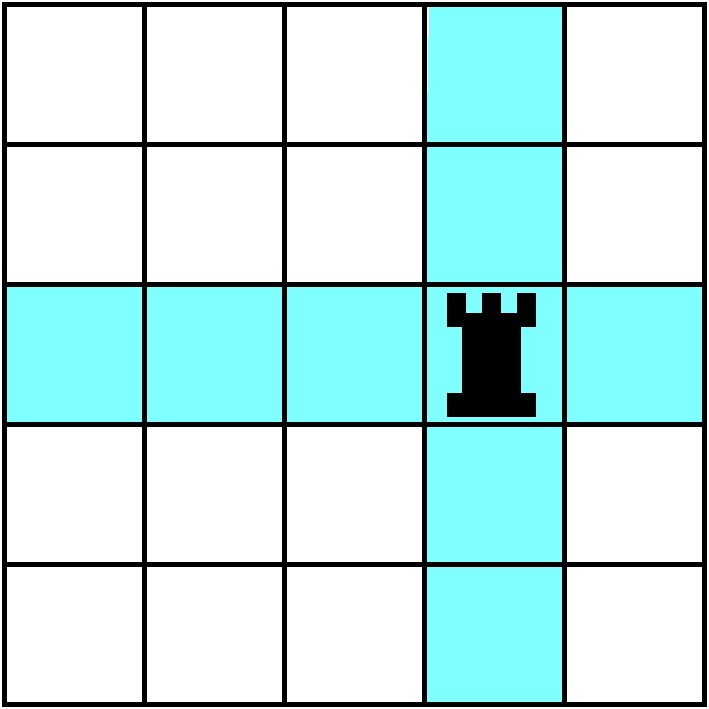
Let's play chess. Only my board, since I need to think small, will be
5 by 5. One of the important chess pieces is a rook (the piece
that usually looks like a castle tower, I think). A traditional chess
problem (problems in chess can be distinct from playing the game,
itself -- they are seen as a skill-sharpening opportunity) is to put
as many rooks as possible on a chess board so that the rooks are
mutually non-attacking. Rooks move across (rows) and down
(columns). They can go any distance. So, in the first picture shown,
we could not put any more rooks down in the colored squares.
Rook arrangements
What's the maximum number of mutually non-attacking rooks we can put
on a 5 by 5 square? We couldn't put more than one in each column and
each row, but ... we can in fact put exactly one in each column and
each row. What's shown is an example of such a rook arrangement (RA).
We can analyze a RA, and try to determine how many RA's there are. I
will count the number of RA's by "constructing" 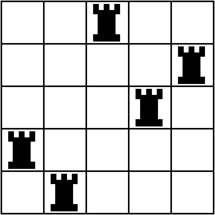 them
column-by-column. We could put a rook in the first column in any of 5
places. Once placed, that rook eliminates its row, and we have only
4 places to put the second rook in the second column. That rook also
eliminates a rook, and there are now 3 places left in the third
column. Similarly there will be 2 places left in the fourth column,
and only one "safe" square in the last column. So there are
5·4·3·2·1=5!=120 different RA's on this 5
by 5 chessboard. I can try to understand the RA I have illustrated by
listing from the top row to the bottom the matrix positions that the
rooks occupy: they are (1,3),(2,5),(3,4),(4,1), and (5,2). In fact,
even in this list this is information which we can discard. We
probably don't need most of the actual parentheses, and, if we agree
that we are reporting the results row-by-row, we don't need the first
coordinates. So the location of the rooks is totally specified by
(3,5,4,1,2). Such an object is called a permutation of the
integers 1 through 5. There are even and odd permutations according to
how many reversals the permutation has. For example, 3 has two
reversals: numbers after it (1 and 2) which are less than it. 5 has
three reversals: the numbers 4 and 1 and 2 appear after it and are
less than it. 4 here has two reversals: 1 and 2, less than 4 and
appearing after 4. 1 and 2 have no reversals. The sum, counting all
reversals, is 2+3+2+0+0 is 7, so this is an odd
permutation. Geometrically, this number counts the positions that are
occupied by rooks below and to the left of rooks on the board. You can
check this. The signature is the number of reversals. If you
now give Maple the following symbolic determinant to compute:
them
column-by-column. We could put a rook in the first column in any of 5
places. Once placed, that rook eliminates its row, and we have only
4 places to put the second rook in the second column. That rook also
eliminates a rook, and there are now 3 places left in the third
column. Similarly there will be 2 places left in the fourth column,
and only one "safe" square in the last column. So there are
5·4·3·2·1=5!=120 different RA's on this 5
by 5 chessboard. I can try to understand the RA I have illustrated by
listing from the top row to the bottom the matrix positions that the
rooks occupy: they are (1,3),(2,5),(3,4),(4,1), and (5,2). In fact,
even in this list this is information which we can discard. We
probably don't need most of the actual parentheses, and, if we agree
that we are reporting the results row-by-row, we don't need the first
coordinates. So the location of the rooks is totally specified by
(3,5,4,1,2). Such an object is called a permutation of the
integers 1 through 5. There are even and odd permutations according to
how many reversals the permutation has. For example, 3 has two
reversals: numbers after it (1 and 2) which are less than it. 5 has
three reversals: the numbers 4 and 1 and 2 appear after it and are
less than it. 4 here has two reversals: 1 and 2, less than 4 and
appearing after 4. 1 and 2 have no reversals. The sum, counting all
reversals, is 2+3+2+0+0 is 7, so this is an odd
permutation. Geometrically, this number counts the positions that are
occupied by rooks below and to the left of rooks on the board. You can
check this. The signature is the number of reversals. If you
now give Maple the following symbolic determinant to compute:
(0 0 a 0 0)
(0 0 0 0 b)
(0 0 0 c 0)
(d 0 0 0 0)
(0 e 0 0 0)
the result will be -abcde. It turns out that the determinant of a matrix with just a "rook arrangement" of positions occupied will always be (-1)# of reversals(the product of the positions). If the signature is even, then the (-1)even is +1, and if it is odd, then the sign will be -. Now here is the official definition of determinant:
The determinant of an n by n matrix A=(aij) is the SUM over all n! permutations p of:
(-1)# of reversals of pa1p(1)2p(2)a3p(3)...anp(n)
Just so maybe you understand how unwieldy this is, for a 10 by 10 matrix, the SUM has 10!=3,628,800 terms, and each of the terms has a sign (+ or -) and is obtained by taking the product of 10 entries in the matrix. This is almost ludicrous computation. But the determinants of much bigger matrices can be and are computed easily (in time proportional to n2, not to some superexponential growth). By the way, the "rules" for computing the determinants of 2 by 2 and 3 by 3 matrices which were so marvelously illustrated last time are clever methods to put the correct signs in front of each product. I don't know any methods for the 24 products involved in the definition of a 4 by 4 matrix.
A very very very special case
 What if a
matrix is upper triangular? That is, everything "below" and to
the left of the main diagonal is 0? To be precise, an n by n matrix
A=(aij) is upper triangular if aij=0 when
j<i. What does the definition of determinant tell us? If we consider
any RA whose position in the first column is other than
a11, the corresponding product will be 0. Now go to the
second column. Since the first column's rook is in the first row, the
second column's rook must be in a row below the first. But if a RA has
the rook below the second row in the second column, that corresponding
product will be 0. So the only position that matters is
a22. Etc. The only RA which contributes to the determinant
of an upper triangular matrix is the product of the diagonal
elements. That is, instead of looking at n! different products, we
only need to look at one:
a11a22a33...ann. The
associated sign is +, since there are no reversals. Therefore the
determinant of an upper triangular matrix is just the product of the
diagonal elements. Now I want to convince you that this "very very
very special case" is actually not a very special case, but a very
good, very practical way to compute determinants.
What if a
matrix is upper triangular? That is, everything "below" and to
the left of the main diagonal is 0? To be precise, an n by n matrix
A=(aij) is upper triangular if aij=0 when
j<i. What does the definition of determinant tell us? If we consider
any RA whose position in the first column is other than
a11, the corresponding product will be 0. Now go to the
second column. Since the first column's rook is in the first row, the
second column's rook must be in a row below the first. But if a RA has
the rook below the second row in the second column, that corresponding
product will be 0. So the only position that matters is
a22. Etc. The only RA which contributes to the determinant
of an upper triangular matrix is the product of the diagonal
elements. That is, instead of looking at n! different products, we
only need to look at one:
a11a22a33...ann. The
associated sign is +, since there are no reversals. Therefore the
determinant of an upper triangular matrix is just the product of the
diagonal elements. Now I want to convince you that this "very very
very special case" is actually not a very special case, but a very
good, very practical way to compute determinants.
Example
Yesterday's QotD again:
(4 1 0 1) (4   1 0    1) (4 1    0    1) (4 1    0    1)
(0 2 1 1)~(0   2 1    1)~(0 2    1    1)~(0 2    1    1)
(1 1 0 0) (0 3/4 0 -1/4) (0 0 -3/8 -5/8) (0 0 -3/8 -5/8)
(0 0 2 2) (0   0 2    2) (0 0    2    2) (0 0    0 -4/3)
Now multiply the diagonal elements: (4)(2)(-3/8)(-4/3)=4. All I did was row operations to "clear" the low-triangular elements to 0. This is easy. The needed work for this is proportional to n2, and is therefore much less than using the definition (which would involve n! amount of work).
Minors, cofactors, row and column expansions, etc.
O.k., suppose we look at the official definition of determinant
again. I'll try to explain why the method called "expanding along the
first column" works.
What can we say about the products in the definition which use
a11? We
must select RA's which don't use the first row and first column. This
means we take the original matrix, and delete the first row and first
column, and look in that matrix for rook arrangements, and we
compute determinant of that matrix. So the
products which involve a11 are just
a11det(M11) where M11 is exactly the
matrix gotten by deleting the first row and column.
What about the
products in the definition involving a12, the second
element on the first
row? If we delete the first row and second column, we must make RA's
in that matrix. So we will compute det(M12). Notice,
though, that in selecting a12 there will always be a
rook below and to the left of the 12 position, so there will always be
a - sign. Therefore the contribution will be
-a12det(M12).
Etc.: for a13 there are
two "rooks" below and to the right of a13 and therefore the
contribution is (-1)2det(M13).
In fact, the determinant of A must be the SUM of
(-1)1+ja1jdet(M1j). Here
Mij is the result of deleting the ith row and
jth column from the n by n matrix. We write the determinant
of an n by n matrix as a sum of determinants of (n-1) by (n-1)
matrices. This leads to methods for evaluating determinants. I will
state the methods both for rows and columns.
Evaluating a determinant by "expanding" along a row
If A is an n by n matrix and i is some integer between 1 and n, then
det(A)=the SUM as j runs from 1 to n of
(-1)i+jdet(Mij) where Mij is the
result of deleting the ith row and jth column
from the n by n matrix, A. Mij is called the
ijth minor of A. The method is called "evaluating the
determinant by expanding along the ith row".
Evaluating a determinant by "expanding" along a column
If A is an n by n matrix and j is some integer between 1 and n, then
det(A)=the SUM as i runs from 1 to nof
(-1)i+jdet(Mij) where Mij is the
result of deleting the ith row and jth column
from the n by n matrix, A. Mij is called the
ijth minor of A. The method is called "evaluating the
determinant by expanding along the jth column".
The important thing to keep track of is the pattern of signs. The signs start at +1 in the upper left corner, and alternate at each vertical or horizontal step:
(+ - + - + - + - + - + - ...)
(- + - + - + - + - + - + ...)
(+ - + - + - + - + - + - ...)
(- + - + - + - + - + - + ...)
(+ - + - + - + - + - + - ...)
(- + - + - + - + - + - + ...)
(+ - + - + - + - + - + - ...)
(...........................)
(...........................)
Examples
Let's take our favorite:
(4 1 0 1)
(0 2 1 1)
(1 1 0 0)
(0 0 2 2)
I asked students what row they would like to use, and was told: "the third".
Third row expansion
   (4 1 0 1)
det(0 2 1 1)=+1det(M31)-1det(M32)+0det(M33)-0det(M34)
   (1 1 0 0)
   (0 0 2 2)
Now consider:
            (1 0 1)                     (4 0 1)
det(M31)=det(2 1 1)=4+4-2=6; det(M32)=det(1 0 0)=0+0+2=2.
            (0 2 2)                     (0 2 2)
I used the special rule for 3 by 3 matrices, but
one can continue to expand along etc. The final result is
1(6)-1(2)=4, as it should be.I think we then did the third column expansion.
Third column expansion
   (4 1 0 1)
det(0 2 1 1)=+0det(M13)-1det(M23)+0det(M33)-2det(M34)
   (1 1 0 0)
   (0 0 2 2)
And:
            (4 1 1)                   (4 1 1)
det(M23)=det(1 1 0)=2(4)=8; det(M34)=det(0 2 1)=-1-5=-6.
            (0 0 2)                   (1 1 0)
so that det(A)=-1(8)-2(-6)=4. I evaluated the first det by expanding
along the third row, and the second det by using the spcial rule for 3
by 3 matrices.
I have found that expanding along a row or column is sometimes useful when dealing with sparse matrices, those with relatively few non-zero entries. But, generally, I convert to upper-triangular form and take the product of the diagonal elements.
A recursive definition
Everybody should try to write a determinant program in a computer
language allowing recursion. Here's an outline:
Entry An n by n matrix A.
If n=1, det(A)=a11.
If n>1, then
det(A)=SUM, as j runs from 1 to n, of (-1)1+ja1jdet(M1j)
Exit Return det(A).
What I've found is that the stack, where stuff gets stored as
recursive calls are made, gets full quite quickly. Oh well.
Historical note
There are many ways of evaluating determinants, because efficient
determinant computation is important. I remark that Dodgson
condensation,
suggested by the English mathematician, Charles
Lutwidge Dodgson, is one interesting method. Also written by the
same author is:
'Twas brillig, and the slithy toves
Did gyre and gimble in the wabe;
All mimsy were the borogoves,
And the mome raths outgrabe.
This was written using the pseudonym, Lewis Carroll.
Transpose
I defined the transpose of a matrix, A. This is At, and
Atij is Aji.
Therefore the transpose of
(2  0  4)
(4 -1 16)
is
(2  4)
(0 -1)
(4 16)
The transpose of a p by q matrix is a q by p matrix, so the transpose of a square matrix is a square matrix of the same size. The following is true, and illustrates the fact that row algorithms and column algorithms will produce the same value for determinant:
IMPORTANT: det(A)=det(At)
This really occurs because in a rook arrangement, the total number of rooks below and to the left is always equal to the total number above and to the right, so the signs will match up, and the # of reversals in A will equal the # of reversals in At (any rook which is below and to the left of another rook has that rook above and to the right!).
Special names
Transpose is used to define special matrices which students may see
here and in other courses.
- Symmetric The matrix A is symmetric if
At=A. Example of a symmetric matrix:
(1 2 3)
(2 0 5)
(3 5 7)
and a non-symmetric matrix:(1 2) (3 4)
If we have a bunch of cities, and aij is the distance from city i to city j, then the matrix of distances will be symmetric. - Skewsymmetric The matrix A is skewsymmetric if
At=-A. Notice that aii then must equal
-aii (if you switch i and i you'll get i and i) so the
diagonal elements of a skewsymmetric matrix are 0.
Example of a skewsymmetric matrix:
( 0  2 -3)
(-2  0  5)
( 3 -5  0)
Example of a matrix which is not skewsymmetric:(0 1 2) (1 4 5) (0 2 2)
If we put n heavy weights on a straight line, and if aij is the force of gravitational attraction directed from weight i to weight j, then the matrix of forces will be skewsymmetric. - Hermitean The matrix A is Hermitean if At is the
complex conjugate of A. Here is a Hermitean matrix:
(   5 2+3i)
(2-3i    5)
The diagonal elements must be real, because the complex conjugates of diagonal elements must be equal to themselves. Hermitean matrices arise in various physical models. - Orthogonal The matrix A is orthogonal if
A-1=At. That is, if you multiply the matrix by
its transpose you get the identity matrix. The matrix
(sqrt(3)/2    1/2  )
( -1/2    sqrt(3)/2)
is orthogonal. The fact that AAt=In implies various facts about inner products. When you take dot products of rows and columns, you get 0 (perpendicular!) except when the row number and the column number agree, when the result is 1: the matrix is a basis of Rn where all the vectors have length 1 and are perpendicular from each other. These matrices will come up in this class later, and they occur in many other places.
The QotD was:
Does the following collection of these 5 vectors in R5 form
a basis:
(5, 2, 1, 0, 0) and (3, 2, 2, 0, -1) and (0, 1, 3, 2, 1) and (2, -2,
2, -2, 2) and (0, 1, 1, 1, 0)?
I told people that they had to work together in groups of 2 or 3, they
could use any computational device, but that they had to
explain their answers.
Please continue reading the text. The homework due at the next meeting is 7.4: 1 and 7.5: 5, 13 and 7.6: 1. Have a good vacation.
March 9
(3 3  3 | 1 0 0) (1  1  1 | 1/3 0 0) (1 0 -1/2 | -1/6 1/2 0)
(3 1  0 | 0 1 0)~(0 -2 -3 |  -1 1 0)~(0 1  3/2 | 1/2 -1/2 0)
(3 0 -1 | 0 0 1) (0 -3 -4 |  -1 0 1) (0 0  1/2 | 1/2 -3/2 1)
and finally
(1 0 -1/2 | -1/6 1/2 0) (1 0 0 | 1/3 -1  1)
(0 1  3/2 | 1/2 -1/2 0)~(0 1 0 |  -1  4 -3)
(0 0  1/2 | 1/2 -3/2 1) (0 0 1 |   1 -3  2)
So
(1/3 -1  1)
( -1  4 -3)
(  1 -3  2)
is the inverse of
(3 3  3)
(3 1  0)
(3 0 -1)
and this can be easily checked by computing the product of the matrices.
The instructor then remarked that the first 6 solutions he read for that QotD were all distinct. Therefore at least 5 of them were incorrect. Ummm ... engineering students should be able to do rational arithmetic.
Let's look at n by n matrices, the nicest matrices. What do we know about these matrices? Square matrices represent systmes of linear equations. If A is such a matrix, then its rank is an integer between 0 and n. What if A is a "full rank" matrix? Then the RREF form of A is In, the n by n identity matrix. What happens?
Matrices which are n by n with rank=n
- AX=0 represents a homogeneous system of n equations in n unknowns. If rank A=n, then the only solution of this system is the trivial solution, where X is the n by 1 column of 0's.
- AX=Y is a system of n equations in n unknowns. If rank A=n, then there are no "compatibility conditions" to be satisfied: the system is always consistent and there is a solution X for every Y. And actually, there is exactly one solution, since if AX1=Y and AX2=Y then (subtracting and undistributing) we know that A(X1-X2)=0 and since X1-X2 is the trivial solution (0) X1=X2.
- The rows of the matrix A are linearly independent if rank A=n. Since the rows are vectors in Rn this means we have n linearly independent vectors in Rn, and the rows form a basis: every vector in Rn can be written as a unique linear combination of the rows. (The same can be said about the columns, actually, but this is a row-oriented course since the text is a row-oriented book).
So square matrices having largest rank are very good. We will discuss determinant. If A is an n by n matrix, then det(A) will be a real number. This number is 0 exactly when the rank of A is less than n. So the value of det(A) could serve as a diagnostic for when the rank=n, if we know how to calculate det(A). When A is 2 by 2 or when it is 3 by 3 there are rather simple recipes for det(A). I want to understand what det(A) means and how to compute it for n larger than 3.
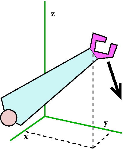 Why does one need det(A) for n>3, anyway? Here's an idea I
got from Professor
Komarova, who is teaching section 1 of Math 421. I hope that M&AE
students will appreciate this example. Think of a robot arm (as
excellently pictured). What information is needed to understand the
"state" of the end of the arm? The word "state" is used here in terms
of control theory. We need to know the position (x and y and z
coordinates) and, also, if the arm is moving (the arrow in the
picture), we would probably also like to record the velocity of the
end of the arm, and that's a vector with three components: already we
are up to R6 for the "state space" of the end of the robot
arm! And there may be more complications, such as a joint or two on
the arm, etc. While it may be obvious how to record the state of the
arm, there may be more advantageous points of view, such as using
something on the robot as the origin of the system of coordinates
(recording data with respect to the robot itself). Then the problem of
changing coordinates occurs, from one system (the "absolute" xyz
system) and the local system of the robot. Typically n by n invertible
matrices and their inverses will be used. And the n might be larger
than we might guess.
Why does one need det(A) for n>3, anyway? Here's an idea I
got from Professor
Komarova, who is teaching section 1 of Math 421. I hope that M&AE
students will appreciate this example. Think of a robot arm (as
excellently pictured). What information is needed to understand the
"state" of the end of the arm? The word "state" is used here in terms
of control theory. We need to know the position (x and y and z
coordinates) and, also, if the arm is moving (the arrow in the
picture), we would probably also like to record the velocity of the
end of the arm, and that's a vector with three components: already we
are up to R6 for the "state space" of the end of the robot
arm! And there may be more complications, such as a joint or two on
the arm, etc. While it may be obvious how to record the state of the
arm, there may be more advantageous points of view, such as using
something on the robot as the origin of the system of coordinates
(recording data with respect to the robot itself). Then the problem of
changing coordinates occurs, from one system (the "absolute" xyz
system) and the local system of the robot. Typically n by n invertible
matrices and their inverses will be used. And the n might be larger
than we might guess.
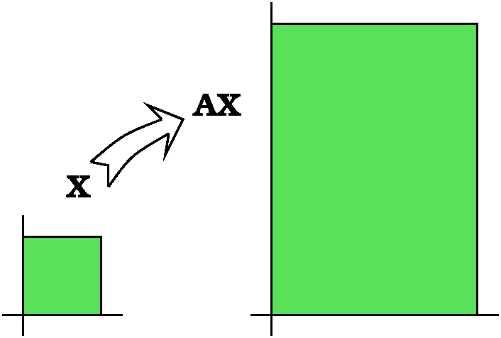
I am going to take a phenomenogical approach to determinants. That is, according to the Oxford English Dictionary, I will deal "with the description or classification of phenomena, not with their explanation or cause." So I will try to describe properties of determinants, and only vaguely hint at the connections between the properties -- how they logically depend on each other. Determinants are quite complicated, and a detailed explanation of what I will show you would probably take weeks! So I will start with an n by n matrix A, which does the following: if X is a vector in Rn, then AX is another vector in Rn. So left multiplication by A is a function from Rn to Rn, taking n-dimensional vectors to n-dimensional vectors (the vectors are column vectors here, of course).
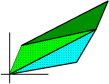
Determinants and geometry
Take the n-dimensional unit cube in Rn. Then the
determinant of A, det(A), is the oriented n-dimensional volume of the
image of the unit cube in Rn under left multiplication by
A.
There are probably words and phrases in this "definition" that you
don't understand. I will try to explain them by looking at some
examples, first for n=2.
 Example 1 Suppose that A is
(2 0)
(0 3)
Then the n-dimensional unit cube is just the two-dimensional square whose corners are (0,0) and (1,0) and (1,1) and (0,1). That part is easy. What happens when we look at A(the unit square)? In this case we get a nice rectangle with corners (0,0) and (2,0) and (2,3) and (0,3). In class I made quite a production of this, and I constantly reminded people that we were dealing with matrix multiplication by A so everything was linear. Therefore A(the unit cube) in two dimensions will always be something "linear", indeed, a parallelogram with one vertex (0,0) etc. It can't be a circle! (It could be a line segment or a point, though: "degenerate parallelograms". You should be able to give A's which transform the unit square to a line segment or a point.) The area of a 2 by 3 rectangle is 6, so det(A)=6 for this matrix.
 Example 2 Suppose that A is
(0 1)
(1 0)
Then the unit square becomes ... the unit square? Well, not exactly. The situation is too darn symmetric to see what happens. Suppose I draw a block F in the square and I very carefully try to compare the domain and range versions of the F. Note that this A takes the i unit vector along the x-axis and changes it to j. And then it takes j and changes it to i. The "positive" angle from i to j (positive is counterclockwise) to "negative" (counterclockwise). While I can look down at the plane and read the F on the left, there is no way (!) I can "read" the F on the right! This A reverses orientation, and its determinant will therefore be negative. Since the geometric area is not changed, the determinant is -1.
 Example 3 Suppose that A is
(1 LARGE #)
(0    1   )
where LARGE # is indeed some really large positive number. This is an example I would be reluctant to show in a beginning linear algebra course, since it is confusing. This mapping distorts distances a great deal (the vertical sides of the square in the domain are 1 unit long, and the corresponding edges in the range are >LARGE #). However, what is amazing is that the area distortion factor is 1. The unit square gets changed to a parallelogram of area 1 (base and height are both 1, after all). This somewhat paradoxical A is an example of a 2-dimensional shear. Notice that the orientation is preserved: although the F is distorted, I can still read it without "flipping" it. This A has determinant 1.
Notice that since these mappings are LINEAR all the areas are distorted by the same factor. That is, if A is a matrix which changes the square's area by multiplying it by 23, then the area of any other region will also be multiplied by 23. In fact, if you think carefully about the area of the unit square first when it is transformed A and then by another matrix, B, then you can see that the compound change in area is det(B)det(A). But we are just multiplying the column vector X first by A and then by B: B(AX). Matrix multiplication is associative, and B(AX)=(BA)X. If you think even more, you can see that det(BA)=det(B)det(A). Amazing! This is useful if we can write a weird matrix as a product of simpler ones, and then compute the determinants of the simpler matrices. There are some real-world algorithms which use this approach.
The determinant is positive if it keeps the same orientation, and it is negative if it reverses orientation. My geometric "intuition" is not particularly good in dimension 23 (it barely works in 1 or 2 or 3!) so I can't really tell you what orientation looks like there. In dimension 3, the determinant of A turns out to be equal to: [(row 1)x(row 2)]·(row 3) if you think about the rows of A as three-dimensional vectors. Here x and · are cross and dot products in R3. Sometimes with specific examples of triples of vectors you can "see" the reversal of orientation, but it can be complicated.
 Now I asked people to try to see the geometry of det(A) in 3
dimensions. The unit cube is changed into a parallelopiped (that's
what it is called!) with one vertex at 0. The oriented volume of that
object is det(A). There are now a wider variety of examples with
det(A)=0. The first example I was given was the all 0's matrix, which
I said was not particularly creative. How about
Now I asked people to try to see the geometry of det(A) in 3
dimensions. The unit cube is changed into a parallelopiped (that's
what it is called!) with one vertex at 0. The oriented volume of that
object is det(A). There are now a wider variety of examples with
det(A)=0. The first example I was given was the all 0's matrix, which
I said was not particularly creative. How about
(1 1 1)
(1 1 1)
(1 1 1)
I was asked? Well, this is a degenerate (!) three dimensional object. Indeed, if you think about it, what you get is the collection of vectors (t,t,t) where t is in [0,1]. This object is 1 dimensional, and its three-dimensional volume is 0, so this determinant must be 0.
Maybe slightly more complicated is
(1 1 1)
(1 0 1)
(1 1 1)
where the image in R3 is a tilted parallelogram, a two-dimensional object: one edge is (1,1,1) and the other is (1,0,1). This object also has three-dimensional volume equal to 0, so the determinant of this matrix is 0.
The two matrices have rank 2 and 1, respectively. These numbers are the same as the dimension count of the image of the unit cube.
Determinants and row operations
There are three row operations which are useful:
- Multiplying a row by a constant.
- Adding a row to another row.
- Interchanging rows.
 What about the second row operation? In two dimensions, we could start
with
What about the second row operation? In two dimensions, we could start
with
(a11 a12)
(a21 a22)
The lower two triangles in the picture to the right represent the image parallelogram. If we add the second row to the first row, the result is
(a11+a21 a12+a22)
(  a21    a22  )
Careful observation will show you that the diagonal of the first parallelogram now becomes a side of the "new" parallelogram. The top two triangles are the new one, and basic geometry should convince you that the areas of the two parallelograms don't change. So adding one row to another doesn't change the determinant, and even adding a multiple of one row to another doesn't change the determinant.
What happens when you interchange rows? Here the mystery of orientation intervenes, just as in example 2 above. The sign of the determinant flips, from + to - or from - to +. There's a sign change.
| Row operation | Effect on determinant |
|---|---|
| Multiply a row by a constant. | Multiply det's value by that constant. |
| Add a multiple of a row to another row. | No change in det's value. |
| Interchange rows. | Change the sign of det. |
Example
I computed the determinant of
(0 2 1 1)
(2 1 1 0)
(1 1 1 2)
(2 0 2 0)
Step 1 Exchange rows 1 and 3. REMEMBER -1.
(1 1 1 2)
(2 1 1 0)
(0 2 1 1)
(2 0 2 0)
Step 2 Use multiples of row 1 to clear the remainder of the first column. Nothing to "remember".
(1  1  1  2)
(0 -1 -1 -4)
(0  2  1  1)
(0 -2  0 -4)
Step 3 Multiply row 2 by -1. REMEMBER -1.
(1  1 1  2)
(0  1 1  4)
(0  2 1  1)
(0 -2 0 -4)
Step 4 Use multiples of row 2 to clear the remainder of the second column. Nothing to "remember".
(1 0  0 -2)
(0  1  1   4)
(0  0 -1  -7)
(0  0  2  4)
Step 5 Multiply row 3 by -1. REMEMBER -1.
(1 0 0 -2)
(0  1 1   4)
(0  0 1   7)
(0  0 2  4)
Step 6 Use multiples of row 3 to clear the remainder of the third column. Nothing to "remember".
(1 0 0  -2)
(0 1 0  -3)
(0 0 1   7)
(0 0 0 -10)
Step 7 Multiply row 3 by -1/10. REMEMBER -10.
(1 0 0 -2)
(0 1 0 -3)
(0 0 1  7)
(0 0 0  1)
Step 8 Use multiples of row 4 to clear the remainder of the fourth column. Nothing to "remember".
(1 0 0 0)
(0 1 0 0)
(0 0 1 0)
(0 0 0 1)
Clearly (yeah, I think in this case, "clearly" is appropriate!) the result has determinant 1. The determinant of the original matrix is the product of all of the REMEMBER notes: (-1)(-1)(-1)(-10). So the value of the determinant is 10. By the way, thank goodness, Maple agrees.
It will turn out that I did some extra, unnecessary work here. It is enough to convert the matrix into "upper triangular" form and then take the product of the diagonal entries. We will see this next time. So come to class!
 In dimension 2, we learn early on that the determinant of
(a11 a12)
(a21 a22)
is +a11a22-a21 a12. The picture indicates this.
In dimension 3, we learn early on that the determinant of
(a11 a12 a13)
(a21 a22 a23)
(a31 a32 a33)
is three positive products of three terms and three negative products of three terms: +a11a22a33+a12a23a31+a13a21a32-a13a22a31-a11a23a32-a12a21a33 The picture indicates this. Maybe: if you can understand the picture (the northwest-southeast products are positive and the northeast-southwest products are negative).
As I mentioned in class, the number of products goes up. It starts 2 and 6, and then ... 24 ... 120, and is n! products of n terms with signs. n! is approximately sqrt(2PI*n)(n/e)n (Stirling's formula), as I said in class, and you can see this grows quickly. 10! is about three and a half million, so a formula like the two above for 10 by 10 matrices would have three and a half million terms. Gaussian elimination is efficient and fast for handling matrices of numbers, but evaluating symbolic determinants efficiently is a current research problem.
I again mention: rows/columns are the same. Anything we're doing with rows is valid and correct for columns.
The QotD was compute the determinant of
(4 1 0 1)
(0 2 1 1)
(1 1 0 0)
(0 0 2 2)
using row operations as shown in this lecture. The answer, I declared, was 4. I hope people got 4. There are lots and lots and lots of algorithms for determinants. Next time we'll look at the official definition, and cofactor expansions.