Return to LFT's
Properties of LFT's
Angle preservation
{Lines/circles}
Triply transitive
Examples
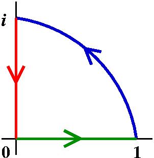
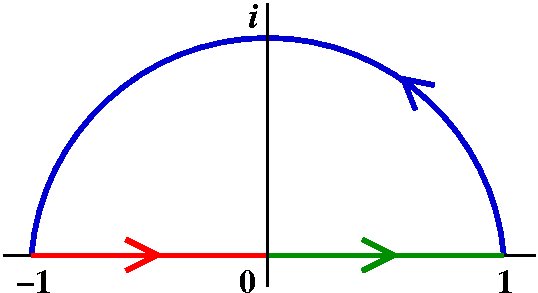
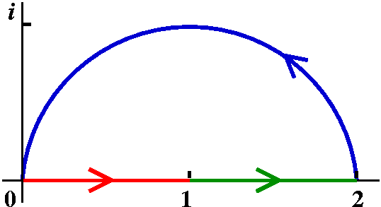
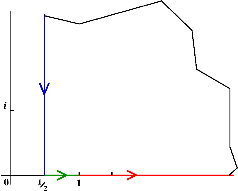
| Start |
|
| z-->z2 |
|
| z-->z+1 |
|
| z-->1/z |
|
| z-->z-1/2 |
|
| z-->z2 |
|
| z-->(-z+i)/(z+i) |
|
 |
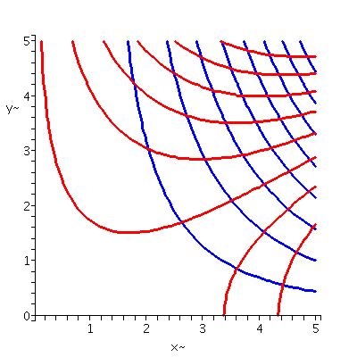 | |
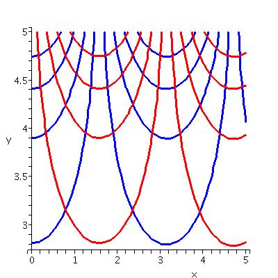
| Contour lines of the real and imaginary parts of sine in the square [0,5]x[0,5]. | Contour lines of the real and imaginary parts of z3-2z in the square [0,5]x[0,5]. |
Techniques in Math 421 and Math 423 (separation of variables, polar coordinates, Fourier series) give very effective methods for computing solutions to the Dirichlet problem in a rectangle or a disc. What about other regions? Something really clever helps.
Transporting solutions to the Dirichlet problem
Well, suppose that we can solve the Dirichlet problem on a domain
R2: we have a steady-state temperature temperature
distribution h. h is a harmonic function, and therefore, at least
locally by our argument above, is the real part of an analytic
function, maybe let's call it g.Now suppose we can map another
domain R1 to R2 by an analytic function f. Look
at h(f(z)) on R1. This is the real part of g(f(z)), which
is analytic, and since the real part of an analytic function is
harmonic, we have just "solved" the Dirichlet problem on
R1.
![]()
In fact, this is what people usually do. They take the "problem" and
the boundary data on a complicated or strange domain and try to change
it into boundary data on a known domain using an analytic function.
Conformal mapping and a BIG theorem
The analytic functions which are usually used in connection with the
Dirichlet problem are also called conformal mappings: they are
1-1 onto functions from a domain R1 to R2. The
known or reference domain which is usually used is the unit disc. The
reason for this is the following result:
The Riemann mapping theorem
Any simply connected domain in C which is not all of C can be
conformally mapped to the unit disc: so there is a 1-1 and onto
analytic function from the domain to the unit disc.
Comment We must exclude C itself from consideration,
because any analytic mapping from C to the unit disc must be constant
by Liouville's Theorem. Weird stuff.
There are no easy proofs of the Riemann mapping theorem. It seems to be a seriously deep result. Also, the theorem is really what's called an existence theorem: there exists a mapping. Maybe we can't readily find the mapping or maybe the mapping isn't really computable or maybe ... Although the Riemann mapping theorem is a major result, so knowing it makes the search for the desired conformal mapping not completely silly, the search may not be too successful.
My last task in this course is to show you some conformal mappings. The most commonly used mappings are the power functions and the linear fractional transformations.
za
LFT
Why the weird condition? (Linear algebra)
A group
How many are there?
Lines and circles
Diary entry in progress! More to
come.
Counting zeros, again
What is multiplicity?
A formula from the Residue theorem
Rouché's Theorem
A simple example
A more complicated example
Mapping
What it's not!
Diary entry in progress! More to
come.
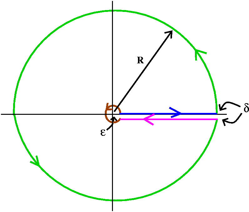
![]() 0infinity[sqrt(x)/(x2+a2]dx=[Pi/sqrt(2a)].
0infinity[sqrt(x)/(x2+a2]dx=[Pi/sqrt(2a)].
This integral is evaluated by using the Residue Theorem applied to the
function f(z)=[sqrt(z)/(z2+a2] on a version of
the famous "keyhole" contour shown. Weird and wonderful contours like
this are well-known in problems coming from physics and from areas in
mathematics (analytic number theory being one of the important
sources). The contour is almost forced by the nature of the function
f(z). The sqrt(z) on the top is a function which is not analytic in
any domain which goes completely around 0. So we need to be
careful. The curve shown is governed by 3 parameters, epsilon, a small
positive number making a curve which is almost a complete circle
around 0; delta, a small positive number separating two straight line
segments, one on the real axis from epsilon to R and one parallel but
slightly below the real axis, and finally almost a complete circle of
radius R, where R is a very large positive number.
I will split up the evaluation along 4 pieces. Then I will evaluate
the residue(s) that I need. And finally I will get the predicted
answer (I hope!).
Diary entry in progress! More to
come.
Fourier transform
The Fourier transform is a clever idea. It changes ordinary and
partial differentiation to multiplication by monomials, so it offers
the possibility that ODE's and PDE's can be solved by algebraic
manipulation. Also, Fourier transform takes "rough" functions,
functions which are just integrable, say, and turns them into analytic
functions (yes, there are some necessary hypotheses, but I am trying
to give the big picture). So manipulating these rough functions, which
can be difficult, can be replaced by working with analytic functions,
which have many nice properties.
One formula defining the Fourier transform is the following:
Suppose f(x) is defined on all of R. Then F(w), the Fourier
transform of f(x), is (1/sqrt{2Pi})![]() -infinityinfinityeiwxf(x) dx.
If you have never seen this before, it looks very weird. It also won't
help if I report, truthfully, that the constants (1/sqrt{2Pi}) and 1
(there's a multiplicative 1 in the exponent) are replaced by other
constants depending on the textbook and the application. Learning the
physics and engineering behind the definition makes it more
understandable (the Fourier transform goes from the "time domain" to
the "frequency domain" etc.) Complex analysis can be used to both
compute explicit Fourier transforms and to analyze the situations
which occur when ODE's and PDE's go throught the Fourier machine.
-infinityinfinityeiwxf(x) dx.
If you have never seen this before, it looks very weird. It also won't
help if I report, truthfully, that the constants (1/sqrt{2Pi}) and 1
(there's a multiplicative 1 in the exponent) are replaced by other
constants depending on the textbook and the application. Learning the
physics and engineering behind the definition makes it more
understandable (the Fourier transform goes from the "time domain" to
the "frequency domain" etc.) Complex analysis can be used to both
compute explicit Fourier transforms and to analyze the situations
which occur when ODE's and PDE's go throught the Fourier machine.
 A computation of the Fourier transform
If f(x)=1/(1+x2), then F(w)=(1/sqrt{2Pi})![]() -infinityinfinityeiwx/(1+x2) dx.
I will forget about the stuff in front (the (1/sqrt{2Pi}) and I will
notice that eiwx=cos(wx)+isin(wx). Since
1/(1+x2) is even and sine is odd and (-infinity,infinity)
is "balanced", the sine part of the integral is 0. So we need to
evaluate
-infinityinfinityeiwx/(1+x2) dx.
I will forget about the stuff in front (the (1/sqrt{2Pi}) and I will
notice that eiwx=cos(wx)+isin(wx). Since
1/(1+x2) is even and sine is odd and (-infinity,infinity)
is "balanced", the sine part of the integral is 0. So we need to
evaluate ![]() -infinityinfinitycos(wx)/(1+x2) dx.
We will use the Residue Theorem, and use it on the now-standard
contour which is shown. But first we need to figure out what the
analytic function is. This is very tricky. The obvious guess would be
(hey, change x's to z's) cos(wz)/(1+z2). But cosine on the
positive imaginary axis goes exponentially. So we won't be able to get
the nice estimate we need to make the integral over SR-->0
with this choice. The choice that is made is very
tricky. First, restrict to w positive, w>0. Then consider
f(z)=eiwz/(1+z2). If |z|=R, and R is
large (R>1) then on SR, with im(z)>=0, we know
|F(z)|<=eRe(iwz)/(R2-1). But if
z=a+ib, with b>=0, then iwz is -wb+iwa. The
real part is -wb, and this is <=0, so eRe(iwz) is
at most 1. Therefore, |F(z)|<=1/(R2-1) and this combined
with L=2Pi R is enough to make |
-infinityinfinitycos(wx)/(1+x2) dx.
We will use the Residue Theorem, and use it on the now-standard
contour which is shown. But first we need to figure out what the
analytic function is. This is very tricky. The obvious guess would be
(hey, change x's to z's) cos(wz)/(1+z2). But cosine on the
positive imaginary axis goes exponentially. So we won't be able to get
the nice estimate we need to make the integral over SR-->0
with this choice. The choice that is made is very
tricky. First, restrict to w positive, w>0. Then consider
f(z)=eiwz/(1+z2). If |z|=R, and R is
large (R>1) then on SR, with im(z)>=0, we know
|F(z)|<=eRe(iwz)/(R2-1). But if
z=a+ib, with b>=0, then iwz is -wb+iwa. The
real part is -wb, and this is <=0, so eRe(iwz) is
at most 1. Therefore, |F(z)|<=1/(R2-1) and this combined
with L=2Pi R is enough to make |![]() SRF(z) dz|<=(2Pi R)/(R2-1)-->0
as R-->infinity. Now the integral over IR-->the desired
improper integral defining the Fourier transform because when z is
real (z=x) then eiwx/(1+x2)=
(cos(wx)+isin(wx))/(1+x2) which when integrated
gives us what we want. All we need is to find the residue of
F(z)=eiwz/(1+z2) at i and multiply
by 2Pi i. Since 1+z2=(z+i)(z-i)
F(z) has a simple pole at i, and the residue is (multiply by
z-i, find the limit as z-->i)
e-w/(2i). But the result of applying the Residue
Theorem is to see that the value of the desired integral is
2Pii[e-w/(2i)]=2Pi e-w. This
is correct for w>0. Generally, the answer will be that the Fourier
transform will be 2Pi e-|w|.
SRF(z) dz|<=(2Pi R)/(R2-1)-->0
as R-->infinity. Now the integral over IR-->the desired
improper integral defining the Fourier transform because when z is
real (z=x) then eiwx/(1+x2)=
(cos(wx)+isin(wx))/(1+x2) which when integrated
gives us what we want. All we need is to find the residue of
F(z)=eiwz/(1+z2) at i and multiply
by 2Pi i. Since 1+z2=(z+i)(z-i)
F(z) has a simple pole at i, and the residue is (multiply by
z-i, find the limit as z-->i)
e-w/(2i). But the result of applying the Residue
Theorem is to see that the value of the desired integral is
2Pii[e-w/(2i)]=2Pi e-w. This
is correct for w>0. Generally, the answer will be that the Fourier
transform will be 2Pi e-|w|.
I wrote again the first three problems from the seventh assignment I
gave in Math 503 last semester:
An example
So we need to compute the integral of
f(z)=1/(z4+a4)2 over
IR+SR when R>a. But f(z) has singularities
exactly where z4+a4=0. By giant thought the
singularities are at eqiPi/4 where q is an integer
and q=1 or q=3 or q=5 or q=4. The only singularities in the upper half
plane occur when q=1 or q=3.
What happens to f(z) at w=eiPi/4? Well, look at
P(z)=z4+a4. I know that P(w)=0, because that is
why we're looking at w. P´(w) is not 0. Why is this? Well,
P´(w)=4z3 and the only place this is 0 is 0 itself,
and that isn't w. Well, here is a very very useful fact:
Proposition Suppose that g(z) is analytic and is not the
zero function. Suppose also that g(w)=0.
This can be really useful, because we all like computing derivatives
(easy) and maybe "factoring" (writing the function as a product with
powers) might not be easy.
Why is this proposition true? Let me try just for k=2. "g(z) has a
zero of order 2 at w" means exactly g(z)=(z-w)2h(z) where
h(w) is not 0. Then g&$180;(z)=2(z-w)h(z)+(z-w)2h´(z),
so g&$180;(w)=0. Of course,
g&$180;&$180;(z)=2h(z)+2(z-w)h´(z)+(z-w)2h´´(z)
so that g&$180;&$180;(w)=2h(w). Thus (as we say in Mathspeak)
g&$180;&$180;(w) is not 0.
On the other hand, if I know that g(w)=g´(w)=0 and
g´´(w) is not 0, look at the Taylor series for g centered at
w. The first non-zero term of this series is the second order term. So
I can factor out (z-w)2, and the other part is a convergent
infinite series with non-zero constant term, which is an analytic
function (h(z)) with h(w) not 0. (The same tricks, again and again!)
Now I know that f(z)=1/(z4+a4)2) has a
double pole, a pole of order 2, at
w=eiPi/4a. Therefore f(z)=(z-w)-2h(z),
where h(z)=A+B(z-w)+higher order terms. B is the residue of f(z) at
w. I tried some really weird way to get B, and was overruled by
students who said: "Multiply and look at the result." So:
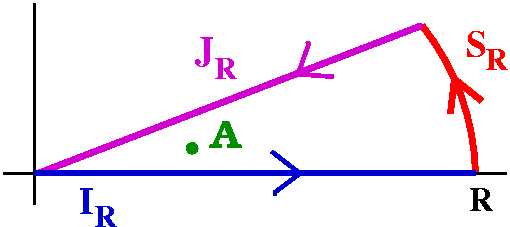
Now In can be computed by residues. It is possible to
compute it with the contour already used, although there will be n
residues to evaluate. Perhaps a more interesting choice of contour is
shown to the right. IR is the interval [0,R] on the real
axis, and as R-->infinity, the integral along IR certainly
approaches In. JR is at angle Pi/n to the real
axis. If z=eiPi/nt, then
z2n=t2n e2IPi=t2n,
and dz=eiPi/ndt, so Notice it is "backwards", and
that as R-->infinity, the integral along JR approaches
-eiPi/nIn. The integral along the
circular SR goes to 0, just using estimates similar to what
we already know.
Now we have (1-eiPi/n)In=2Pii
multiplied by the residue of 1/(1+z2n at the green dot, which is
eiPi/(2n). This is a simple pole, because (just as
before!) the derivative of 1+z2n is 2nz2n-1 and
the two polynomials do not have any roots in common. So we just need
the residue of 1/(1+z2n) at eiPi/(2n),
which is limz-->eiPi/(2n)(z-eiPi/(2n))/(1+z2n).
I use L'Hopital's rule, and get the following as the
value of the limit:
HOMEWORK
On Thursday, I will "review": I will answer questions about the
homework (you should look at 2.6: 3,5,13, 18, 26).
Another point of view
Isolated singularity?
A Laurent series from the textbook
I am treating this as sort of a big polynomial computation. This is
justified because the series converges absolutely and any sort of
rearrangements, etc., are correct. Then we can get the series for
z/[sin(z)]2 by multiplying this by 1/z.
Sigh. Or I can ask Maple:
Is residue additive?
Is residue multiplicative?
A residue
A version of the grown-up Residue Theorem
Suppose f(z) is analytic in a simply connected domain except for a
finite number of isolated singularities. Suppose that C is a simple
closed curve which does not pass through any of the isolated
singularities. Then the integral
Consider the function f(z)=[1/(1+z2)]. This function is
analytic except for two isolated singularities at +/-i. Since
z2+1=(z+i)(z-i), I also know that the isolated
singularities are simple poles (poles of order 1). Indeed, I can
compute the residue of f(z) at i by considering the limit of
(z-i)f(z) as z-->i. This is easy enough, since (z-i)f(z)=1/(z+i).
The residue is therefore 1/[2i]. But how can I use this to compute
the real integral above?
Approximate
Now what happens as R-->infinity? The integral over SR
certainly --)0 and the integral over IR-->the desired real
integral. But the Residue Theorem allows us to compute the integral
over the closed curve as 2Pi i(the residue of f(z) at i), and this
is 2Pi i(1/[2i]) and, WOW!, this is Pi.
A workshop (?)
Exam?
Isolated singularity: the definition
Isolated singularity: here's all you need to know
Example of a ludicrous result
The uselessness of mathematics (Is this
news?
Analyticity in an annulus yields Laurent series
The exposition in the textbook is good (pp. 141-144), and shows how,
given a function f(z) which is analytic in an annulus, then there are
unique complex constants an, for any integer n, so that
f(z) is equal to
SUMn=-infinity+infinityan(z-z0)n.
Here I think the simplest way to understand the doubly infinite sum is
to think of it as the sum to two infinite series. What's really neat
is that this series converges in a manner similar to power series
inside the radius of convergence. That is, it converges absolutely, so
you can do anything algebraic you would like (rearrangement, grouping,
etc.). Also, the series converges uniformly on circles
|z-z0|=t where t is between the inner and outer radius of
the annulus. This means you can "exchange" integral and sum, and not
worry. These properties follow in a similar fashion as they did for
power series. One "expands the Cauchy kernel" and the geometric series
plays a double role, on an inside and an outside circle. I gave a very
rapid, not so good, exposition of the "expanding" process. I think I
got the formula an=
I then applied the properties of Laurent series to get the
characterizations for an isolated singularity. If the isolated
singularity is removable, then consider the formula for the
an's above when n<0. Look at the signs of the power
inside the integral, and see that for negative n's, the integrand is
analytic inside of |z-z0|<r for a removable
singularity.
If f(z) has a pole at z0, then 1/f(z) has a zero there (and
the singularity is removable). Look at the power series for
1/f(z). You can "factor out" the lowest power of z-z0
which appears, and the result is (z-z0)k
multiplying a power series whose constant term is not 0. But
the power series represents an analytic function p(z) with
p(z0) not equal to 0. Therefore
f(z)=[1/(z-z0)]h(z) where h(z)=1/p(z) is analytic near
z0 and which therefore has a power series beginning with a
non-zero constant term. Wow. Then multiply through and get the Laurent
series behavior guaranteed by the table. The Laurent characterization
of essential singularities follows from the fact(s) that the other
Laurent characterizations are "if and only if" -- no negative terms if
and only if removable; finitely many negative terms if and only if pole.
One computation
I found (some of_ the Laurent series for each of the functions in the
table.
The child's residue theorem
The residue of f(z) at z0 is a-1, the
(-1)th coefficient of the Laurent series of f(z) centered
at z0
HOMEWORK
Therefore, if f has a zero of order k at z0 then we can
write f(z)=(z-z0)kg(z), where g(z) is analytic,
and g(z0) is not 0 (so g(z) is not 0 near z0,
actually).
The converse is also true. That is, we can write f(z) as
(z-z0)kg(z), where g(z) is analytic, and
g(z0) is not 0. Then look at the power series for g(z) and
and get the (unique!) pwer series for f(z) centered at
z0. So we reverse the procedure to see that the needed
derivatives of f(z) are 0 until the kth derivative.
It can be much easier to manipulate the function f(z) rather than
compute its derivatives. Although certain people in class did not
believe this, I suggested that we could consider the polynomial
(related to a homework assignment!) f(z)=(z2+z-2)35.
Then surely f(z)=((z-1)(z+2))35=(z-1)35(z+2)35.
Now f(z)=(z-1)35g(z) where g(z)=(z+2)35 so that
g(1)=335 which is not zero. Therefore f(z) has a
zero of order 35 at 1. In a similar fashion, one could conclude that
f(z) has a zero of order 35 at -2. I sincerely doubt that I would want
to verify these statements by direct computation and evaluation of the
first 35 derivatives of f(z).
Well, darn it, I just tried this in Maple on a
Math Department computer which is moderately fast and which has a
rather new version of the program. And I "verified" that f(z) has a
zero of order 35 by direct computation in time much less than a
second. Well, my remark is still correct. Ideas matter. Sigh. So much
for Mr. Canis Lupus.
THIS IS NOT COMPLEX
ANALYSIS SO YOU CAN DISREGARD
IT!
You will never, never, never, consider such a function in a complex
analysis course like Math 403. Our functions are either 0
everywhere or they are zero at isolated points.
The picture was produced using these
commands:
Isolated singularities
REMOVABLE
Such a singularity is called removable: if f(z) has an isolated
singularity at z0 and if there is some way of assigning a
value to f(z) at z0 so that the resulting function is
analytic at and near z0, the singularity of f(z) at
z0 is called removable. Here is a neat result about such
singularities:
Counterexample (?)
Proof
Now we can analyze poles even more closely: if f(z) has an isolated
singularity at z0 and if |f(z)|-->infinity as
z-->z0, then 1/f(z) is bounded near z0 and
1/f(z) has a removable singularity at z0. Therefore
1/f(z)=(z-z0)kh(z) where h(z) is analytic and
h(z00)-k(1/h(z)). So any pole has
its modulus -->infinity like an inverse integer power of
|z_z0
|.
OTHER: "ESSENTIAL SINGULARITIES"
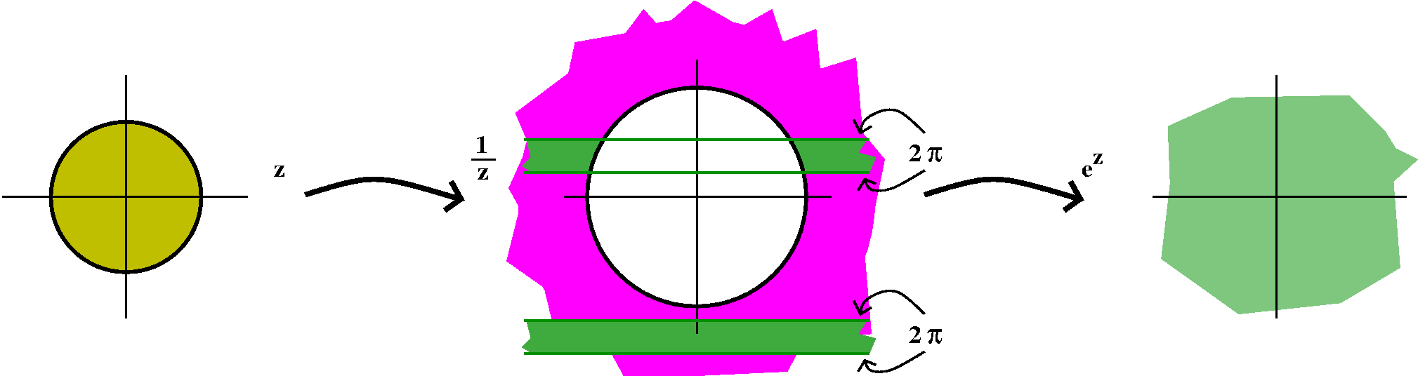
The mapping z-->e1/z is a composition of two mappings. On
a small "deleted" disc centered around 0, the first map, z-->1/z takes
0<|z|<epsilon to the entire exterior of a circle of
radius 1/epsilon. Now we need to look at how this domain is mapped by
z-->ez. Remember that this is the complex exponential
mapping, which is periodic with period 2Pi. And in every horizontal
strip which is 2Pi high, the mapping is onto all of C except
for 0. Certainly there will be some (many!) 2Pi high strips which are
totally contained in the domain |z|>1/epsilon. Therefore the image
will actually be all of C except for 0. The next theorem says
that something similar happens more generally.
Casorati-Weierstrass Theorem
Proof We assume that C-W is not true, and derive a
contradiction. I will finish the proof on Tuesday evening, and also
get some other amazing results.
Last time we learned "another result making
analytic functions equation. We can apply this to
An answer
Radchenko-Bolzano-Weierstrass
The Cauchy estimates
Another exam problem
The first time you see one of these problems there is a great amount
of strangeness. One tries to think of examples. For this estimate,
there certainly are lots of examples, such as z and z2 and
... But then one tries to think of non-polynomial examples, such as
sin(z). But we eliminated sin(z), because while it has rather tame
"growth" on the real axis, if z=iy, then |sin(z)|=|sinh(y)) which
grows exponentially (like (1/2)ey) and can't be boun ded by
poloynomial growth.
In fact, if |f(z)|<=4(1+|z|)10 for all z, then f(z)
must be a polynomial of degree 10 at most. Why? The easiest way to
verify that a function is a polynomial is to differentiate it a bunch
of times and see that the result is identially 0. A function that has
derivative 0 must be a constant. A function whose second derivative is
0 must be linear. A function whose ... In this case, I will prove that
the 11th derivative of f(z) is 0. I will use the Cauchy
estimates with n=11.
So
|f(11)(z0)|<=[11!/r11]max|z-z0|=r|f(z)|.
And another
Liouville ==> Fundamental Theorem of Algebra
Suppose
p(z)=z7+(5+i)z6-4z2+z-9. Then the
main idea is to look at p(z) for |z| large.
|p(z)|=|z|7|1+(5+i)z-1-4z-5+z-6-9z-7|. Now choose |z| large enough. Let me
try |z|>100. Then
If |z|>100, |p(z)|>=|z|7(1/2). Therefore |p(z)|
can't be 0 and in fact, 1/p(z) will have modulus at most
2/(100)7 when |z|>100.
The approach to proving the Fundamental Theorme of Algebra is this: if
p(z) is never 0, look at f(z)=1/p(z). I bet that this is bounded,
hence (Liouville) constant, contradiction because p(z) is certainly
not constant.
The estimate we just verified:
Well consider p(z) on the z's with |z|<=100. If I assume that p(z)
is never 0 (or else we have a root!) then what can I say? Well,
suppose that |p(z)| gets close to 0. In fact, what if there is a
sequence {zn} inside this disc with
|p(zn|<1/n. Then (Bolzano-Weierstrass) there is a
convergent subsequence. That is, we can find a subsequence so that
|p(znk|<1/nk and the
znk-->some number w. But then p(w) has to be 0
since the polynomial p is continuous and p(w) is the limit of the
p(znk)'s. But we are assuming that p has no
roots. Therefore |p(z)| must have a positive minimum inside
|z|<=100. So f(z)=1/p(z) has a positive maximum inside
|z|<=100. Therefore f(z) is eligible for Liouville's Theorem, and
hence we get the contradiction mentioned above.
Outside the disc, use a simple underestimate, and inside the disc, use
Bolzano-Weierstrass to convinced yourself that p(z), if it were to
never be 0, would have a positive minimum in modulus.
Order of the zero of an analytic function
Example
Since f(z)=(cos(z)-1+(1/2)z2)5 and we know the
Taylor series for cos(z) centered at 0, we can write
Too many ideas ... let us reconsider
THIS IS NOT COMPLEX
ANALYSIS SO YOU CAN DISREGARD
IT!
Now to get f2(x). First, I'll double f1(x):
consider 2f1(x). Then let's squeeze it so it will vibrate
twice as fast: 2f1(2x). Now finally let us shift it right
by 2k. Thus, f2(x)=2f1(2[x-2k]). The pictures
below illustrate what I'm doing. (except for the last picture which I
just noticed needs to be moved right another k!).
Well, I will "construct" or indicate how fn+1 should be
defined by a recursive formula:
We now see:
If you would prefer arguments involving functions defined by formulas,
and if you would like to learn more about the mistakes people made
when they began studying Fourier series and power series, one nice
reference at a level appropriate for students in this class is
A Radical Approach to Real Analysis by David Bressoud.
Uniform convergence?
Suppose that we have a sequence of functions, {f_n(x)}, each
continuous and defined on the interval [a,b]. Then we say that
SUMn=1infinityf_n(x) converges
uniformly to F(x) on [a,b] if, given any epsilon>0, there is
an N so that if m>N,
|SUMn=1mf_n(x)-F(x)|<epsilon
for all x on [a,b]. This condition certainly does not hold in the
example previously discussed. But then
And power series almost do that ...
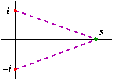
Return to 1/(1+x2)
I know that 1/(1+x2)=A/(x-i)+B/(x+i). Here we can guess
that A=-i/2 and B=i/2 (or you can systematically solve the
partial fraction equations). Now let me look at the first piece.
We know that (i/2)/(x-i)= (i/2)/([x-5]+[5-i]). If x-5 is small, we
can use the geometric series, with r=(x-5)/(5-i). So look:
Well, 1/(1+x2) is just the restiction to R of
1/(1+z2) analytic on all of C everywhere except +/-i. If
you look at the proof we gave last time for the implication
{analytic==>power series} you should see that we can get a power
series for an analytic function up to the first "singularity", the
largest disc so that the function stays analytic in the whole
disc. Here, for 1/(1+z2) and for the center 5, that disc
will have radius sqrt{26}, the distance from 5 to +/-i. In general,
the radius of convergence of the power series for 1/(1+x2)
centered at x0 in R will be
sqrt{1+x02} for the same reason. Therefore this
function is a counterexample to the real version of the
bubbles result I stated last time. The function is equal to a
power series centered at every point, and the radius of convergence is
at least 1. But the function is not equal to a power series with
infinite radius of convergence.
Real/complex: what is the correct idea?
A refreshing break?
What is (or should be) sin(z)?
Derivatives at 0?
One result making analytic functions equal
Analytic functions as infinite degree polynomials
With this as background, maybe we can "force" two analytic functions
to be equal by asking that their values agree at infinitely many
points. Well, things aren't that simple. As suggested by several
students, the entire functions sin(z) and cos(z) agree at infinitely
many points (say, many [not all!] multiples of Pi/4) and certainly are
not the same. But something like this almost works if you ask
for a little bit more.
How to force a function to be sine
Another result making analytic functions equal
To verify this, we just need to show that
f(z0)=g(z0),
f´(z0)=g´(z0),
f´´(z0)=g´´(z0),
f´´´(z0)=g´´´(z0),
etc. because then we can use the previous result.
Why is f(z0)=g(z0)?
Why is f´(z0)=g´(z0)?
Why is
f´´(z0)=g´´(z0)
Why is ....
So what is sine?
How to prove (?!) a trig identity
Analytic continuation
A corollary observed by Mr. Radchenko
Expanding the Cauchy kernel
Interchanging sum and integral
After you do the exchange of sum and integral, and then "recognize"
what you have logically, you will realize that:
Power series forever!
A hard theorem
If you think about this result, it is very puzzling. Somehow some
"thing" is pushing the radius of convergence bigger and bigger
and bigger. I don't know any simple direct proof of this result. But
let's use the machinery that we have:
Counterexample (?)
Zero integrals imply .... (Morera's Theorem)
My empire stretches forever!
There are other equivalences, some of which I will discuss later. To
me the nicest equivalence yet undisclosed has to do with
conformality which I have mentioned earlier.
Liouville's Theorem
On Thursday
HOMEWORK
Maintained by
greenfie@math.rutgers.edu and last modified 1/18/2005.
I'll be in my office Monday afternoon and Tuesday afternoon and will
try to answer questions about the material that the exam will cover.
Tuesday, April 12
(Lecture #21, approximately)
I stated that the Residue Theorem contains all of the integral
formulas which we've seen in this course. This may be an exaggeration,
but not by much. For example, we have the Cauchy Integral Formula for
Derivatives. One example of this formula is the following:
Suppose f(z) is analytic in a simply connected domain, C is a simple
closed curve in the domain, and z0 is a point inside
C. Then f(5)(z0)=[5!/(2Pii)]![]() C[f(z)/(z-z0)6] dz.
C[f(z)/(z-z0)6] dz.
Look at the function g(z)=[f(z)/(z-z0)6]. This
function is analytic in the original domain of f(z) except possibly at
z0, where it has an isolated singularity. But what is the
residue of g(z) at z0? We only need to compute a "local"
Laurent series for g(z) near z0 to answer this. Well, since
f(z) is analytic for z near z0, f(z) must "locally" be the
sum of a power series, and this power series must be the Taylor
series for f(z) at z0:
f(z)=SUMn=0infinity[{f(n)(z0)}/n!](z-z0)n.
Then
g(z)=[f(z)/(z-z0)6]=SUMn=0infinity[{f(n)(z0)}/n!](z-z0)n-6. The residue of g(z) at z0 is just the -1st coefficient in this series. But n-6=-1 when n=5. The coefficient of (z-z0)-1 in the series for g(z) is therefore
[{f(5)(z0)}/5!]. The Residue Theorem then
declares that the integral
![]() Cg(z) dz=
Cg(z) dz=![]() C[f(z)/(z-z0)6] dz=2Pii[{f(5)(z0)}/5!],
and this immediately gives the desired formula.
C[f(z)/(z-z0)6] dz=2Pii[{f(5)(z0)}/5!],
and this immediately gives the desired formula.
These problems are all taken from Theory of Complex Functions
by R. Remmert. They can all be verified using the Residue Theorem. And
now I think that Maple can do them all. There are huge books
with thousands of formulas for definite integrals. Many of the
formulas have Pi's in them. The Pi's almost all come from ... 1/z
integrated around the unit circle and the Residue Theorem. Some
modern references are:
![]() 02Pidq/[a+sin(q)]=[{2Pi}/sqrt(a2-1)]
if a is real and a>1.
02Pidq/[a+sin(q)]=[{2Pi}/sqrt(a2-1)]
if a is real and a>1.
![]() -infinityinfinity
dx/[(x4+a4)2=(3/8)(sqrt(2)/a7)Pi
for a>0.
-infinityinfinity
dx/[(x4+a4)2=(3/8)(sqrt(2)/a7)Pi
for a>0.
![]() 0infinity[sqrt(x)/(x2+a2]dx=[Pi/sqrt(2a)].
0infinity[sqrt(x)/(x2+a2]dx=[Pi/sqrt(2a)].
I tried to verify one of the formulas from my homework assignment last
semester. I chose
![]() -infinityinfinity
dx/[(x4+a4)2=(3/8)(sqrt(2)/a7)Pi
for a>0.
Well, this was a little bit silly because the same picture and
estimates which are in the same style as the example I
did last time will work. So look there, and IR and
SR are the same. We can use ML to show that the
SR integral-->0 as R-->infinity. Why? Well, if |z|=R, then
|z4+a4|>=|z4|-|a4|=|z4-|a|4=R4-a4
(we know a is positive). Therefore if R is sufficiently large
(R>a), f(z)=1/(z4+a4)2,
|f(z)|<=1/(R4-a4)2. And the
SR integral has its modulus bounded by
PiR/(R4-a4)2 which certainly -->0 as
R-->infinity. And the IR integral approaches the improper
integral we want to compute as R-->infinity.
-infinityinfinity
dx/[(x4+a4)2=(3/8)(sqrt(2)/a7)Pi
for a>0.
Well, this was a little bit silly because the same picture and
estimates which are in the same style as the example I
did last time will work. So look there, and IR and
SR are the same. We can use ML to show that the
SR integral-->0 as R-->infinity. Why? Well, if |z|=R, then
|z4+a4|>=|z4|-|a4|=|z4-|a|4=R4-a4
(we know a is positive). Therefore if R is sufficiently large
(R>a), f(z)=1/(z4+a4)2,
|f(z)|<=1/(R4-a4)2. And the
SR integral has its modulus bounded by
PiR/(R4-a4)2 which certainly -->0 as
R-->infinity. And the IR integral approaches the improper
integral we want to compute as R-->infinity.
g(z) has a zero of order k at w if and only
if g and all of its derivatives up to order k-1 are 0 at w
and the kth derivative of g at w is not 0.
(z4+a4)2(A+B(z-w)+higher order terms)=(z-w)2.
Therefore a8Bz is the z term on the right hand side, and
that is -2wz. And
B=-2w/a8=-2eiPi/4a/a8=
-2eiPi/4/a7.
>residue(1/(z^4+a^4)^2,z=exp(I*Pi/4)*a);
1/256*(24*I*2^(1/2)*a^5+24*a^5*2^(1/2))/a^12
>simplify(%);
(-3/32-3/32*I)*2^(1/2)/a^7
Somewhere in this is a mistake. Where is it?
 M. Kalelkar's favorite integral
Mr. J. Walsh came and computed In=![]() 0infinity[1/(1+x2n)dx, where
n is a positive integer. This, I was told, is Professor Kalelkar's
favorite integral. Professor
Kalelkar is a faculty member in the Physics Department, and in
charge of the undergraduate physics program.
0infinity[1/(1+x2n)dx, where
n is a positive integer. This, I was told, is Professor Kalelkar's
favorite integral. Professor
Kalelkar is a faculty member in the Physics Department, and in
charge of the undergraduate physics program.
1/2n(eiPi/(2n))2n-1.
 The answer, and rudimentary checking of the answer
The value of In, after some algebraic manipulation, turns
out to be (Pi/2n)/sin(Pi/2n). You can sort
of check this.
I always try to check complicated formulas if I can. Much of the
time such formulas are easiest to check at the extremes (here
n=1 and n-->infinity).
I'll give an exam a week from today. The exam will cover up to the end
of section 2.6 (use of the Residue Theorem to compute real
integrals). Although the course is cumulative, most questions will
concentrate on what we've done since the last exam. The course home
page has links to various resources (an old exam with answers, and
review material with answers) which should be helpful.
Thursday, April 7
(Lecture #20, approximately)
I reviewed some of the material from the past lecture. Then I
addressed a lovely question asked by Mr. Solway. He remarked that sqrt(z) has a
singularity at 0. What kind of singularity (of the trichotomy)
is it? Mr. Schienberg observed that
sqrt(z) is certainly bounded in 0<|z|<1. Therefore ... the
singularity must be removable.
If sqrt(z) has a removable singularity at 0, then we have an analytic
function f(z) defined in a disc centered at 0 so that
f(z)2=z. But then we can differentiate, and get
2f(z)f´(z)=1 for |z|<1. What if z=0? Well, as z-->0, I think
that sqrt(z)-->0, so f(0)=0. But:
2·0·SOMETHING=1. This can't be true. So where is
the contradiction?
sqrt(z) does not have an isolated singularity at 0. There is no
r>0 so that sqrt(z) is analytic in all of 0<|z|<r.In fact, if
you look at sqrt(z) as it travels "around" a circle, you will see that
when you get back to where you started, the arguments do not match up
(one-half of 2Pi is not the same as 0, mod 2Pi). So there is a need to
be a bit careful.
I believe the textbook asked for the first four terms of the Laurent
series of
z/[sin(z)]2 at 0.
#1Does f(z) have an isolated singularity at 0?
Yes, it does. sin(z) is 0 when z=0 and the nearest "other" zero of
sin(z) is at +/-i.
#2If yes, what type?
I bet it is a pole. I think it is a pole of order 2. Why? Well, I know
that sin(z)=zh(z) where h(z) is an analytic function so that
h(0)=1. h(z) is just the (convergent!) infinite series for sin(z) with
one power of z "factored out".
#3Find some of the Laurent series.
Well, sin(z)=z(1-z2/6+z4/24+...) so that the square of sin(z) is z2(1-z2/3+[(1/62)+[2/48]z4+...). Therefore,
z/[sin(z)]2=(1/z)(
1/[1-z2/3+[(1/62)+[2/48]z4+...]) and I choose to think about the terms inside the
parentheses as a/(1-r) where a=1 and
r=z2/3-[(1/62)+[2/48]z4+...]. Then
a+ar+ar2+... becomes
1+(z2/3+[(1/62)+[2/48]z4+...])+(z2/3+[(1/62)+[2/48]z4+...])2+... and this is
1+z2/3+(something)z4+... where the "something" is
[(1/62)+[2/48]+1/32. Whew!
>series(z/(sin(z))^2,z=0,10);
                -1                 3          5      7
               z   + 1/3 z + 1/15 z  + 2/189 z  + O(z )
Yes. If f(z) and g(z) both have isolated singularities at
z0, then the residue of f(z)+g(z) is equal to the
sum of the residues of f(z) and g(z). That is because the sum of two
Laurent series is a Laurent series, and the only way you can get
the(-1) coefficient is by adding the two (-1) coefficients.
No. Look at f(z)=g(z)=1/z. Then the residues at 0 of both f(z)
and g(z) are each 1, but the residue of f(z)=g(z)=1/z2 at 0
is 0.
I got this example from at old but wonderful textbook by Saks and
Zygmund. The function f(z)=ez+(1/z) has an isolated
singularity at 0. What is the residue of f(z)? Well, since
ez=SUMn=0infinityzn/n!
and
e1/z=SUMn=0infinity1/[znn!]
and everything will "work" we just need to find the coefficient of 1/z
in a purely formal way, just by algebraic manipulation. Everything is
guaranteed to converge. If you keep track of the exponents, and match
everything carefully (as I tried to do in class) then you will see
that the coefficient of 1/z, which is the residue of f(z) at 0, is
SUMn=0infinity1/[n!(n+1)!]. And there is
no wonderful "simplification" -- the real number defined by this sum
is J0(1), a value of a Bessel function. Generally, "finding"
residues and Laurent expansions of functions with essential
singularities is quite difficult especially if "finding" means you can
make sense out the result.
There are many versions of the Residue Theorem. The version in your
textbook (p. 154) is certainly adequate for many routine computations
and applications.![]() Cf(z) dz is 2Pii multiplied by the sum
of the resides at the isolated singularities which lie inside the
curve.
Cf(z) dz is 2Pii multiplied by the sum
of the resides at the isolated singularities which lie inside the
curve.
Note If there are no isolated singulatities then the sum
in the theorem would be empty -- there is nothing to add. In that
case, we should interpret the value of an empty sum to be 0.
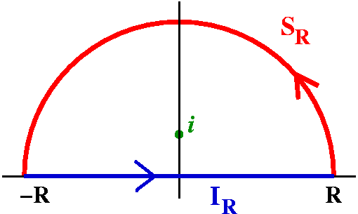
A real integral
The integral I looked as was the definite integral ![]() -infinityinfinity[1/(1+x2)] dx.
If you know that the derivative of the usual arctan function is the
integrand, [1/(1+x2)], and you also know the limiting
values of arctan as x-->+/-infinity, then it's easy to see that he
integral's value is Pi. But: it is generally better to know more ways
to compute things. Sometimes one way will work, and sometimes, another.
-infinityinfinity[1/(1+x2)] dx.
If you know that the derivative of the usual arctan function is the
integrand, [1/(1+x2)], and you also know the limiting
values of arctan as x-->+/-infinity, then it's easy to see that he
integral's value is Pi. But: it is generally better to know more ways
to compute things. Sometimes one way will work, and sometimes, another.
![]() -infinityinfinity[1/(1+x2)] dx
by
-infinityinfinity[1/(1+x2)] dx
by ![]() -RR[1/(1+x2)] dx for R
large. In particular, I want R>1, so that when I look at the
indicated contour (in the picture to the right), i will be inside the
closed curve. The real integral from -R to R is equal to the integral
of the analytic function, f(z), on IR. What about the
integral over the semicircle, SR? We can estimate this
integral using the ML inequality. L is just Pi R. As for M, we
want to get an overestimate of |f(z)| when |z|=R and R>1. But we
can get an overestimate of the quotient by underestimating the
bottom. So:
-RR[1/(1+x2)] dx for R
large. In particular, I want R>1, so that when I look at the
indicated contour (in the picture to the right), i will be inside the
closed curve. The real integral from -R to R is equal to the integral
of the analytic function, f(z), on IR. What about the
integral over the semicircle, SR? We can estimate this
integral using the ML inequality. L is just Pi R. As for M, we
want to get an overestimate of |f(z)| when |z|=R and R>1. But we
can get an overestimate of the quotient by underestimating the
bottom. So:
|z2+1|>|z2|-1=|z|2-1=R2-1.
Therefore the integral over SR has modulus at most
[Pi R]/[R2-1].
I gave out
a workshop problem but didn't have time to go over it.
Real soon.
Tuesday, April 5
(Lecture #19, approximately)
We assume the contradiction: what if C-W is not true. So there
is a>0 and b>0 and w0 in C so that if
|z-z0|<a, then |f(z)-w0|>b. Look at the
function
g(z)=1/(f(z)-w0). So g(z) has an isolated singularity at
z0. But |g(z)|<1/b, so g(z) has a removable singualrity
at
z0 by Riemann's Theorem. So g(z0) hss a
value. Now rewrite, and notice that f(z)=w
f(z) has an isolated singularity at z0 if there is r>0
so that f(z) is analytic in the "deleted disc",
0<|z-z0|<r.
Comments This definiton leads to some silly examples. Let's
see: the function f(z)=z2 has an isolated singularity at,
let's see, -4=5i or, in fact, any z0. That's a
consequence of the language. The examples we "really" want to cover
imply that we need this rather weak definition.
Here's a table with all the entries completed. Please realize that
Inventing" and examining the entries required about 1.5 class meetings
-- quite a lot of time. The most amzing fact is perhaps hidden in the
trichotomous structure of the table itself: any isolated
singularity must be one of the named varieties. There is no other kind
of allowed behavior. This is in sharp contrast with the free situation
in one-variable (real) calculus. There if you know that a function is,
say, differentiable in all of R except 0, all sorts of
weirdness can occur.
Isolated Singularities Name Characteristic example(s) Defining behavior
Relevant theorems
Characterization by Laurent series Removable singularity
[sin(z)]/z at z0=0
There's a way of defining the function, f(z), at the center z0 of the
deleted disc, so that when the f(z) is looked at with this value, the reuslt is
analytic in all of the disc, |z-z0|<r
Riemann's Removable Singularity Theorem
If f(z) is bounded
in 0<|z-z0|<r, then f(z) has a removable singularity at
z0.
"Bounded" means there is a real (positive) M so that |f(z)|<M for all z's
with 0<|z-z0|<rAll of the coefficients in the Laurent
series for f(z) in the deleted disc centered at z0
corresponding to negative integer indices are 0.
The Laurent series is a power series.Pole
7/(z-5)3
1/(ez-1)2 at z0=0.The limit of |f(z)| as z-->z0 is infinity.
That is, given any positive real number M, there is some epsilon>0 so that
if |z-z0|<epsilon, |f(z)|>M.In the deleted disc, f(z)=h(z)/[(z-z0)k, where h(z) is
analytic in the whole disc |z-z0|<r and and h(z0)
is not 0.
k is a positive integer called the order of the pole at z0.Only a finite number of terms in the Laurent series for f(z) in
the deleted disc centered at z0 corresponding to negative
integers are not 0.
You can "factor out" the correct inverse power
of z-z0 from the Laurent series and get
[(z-z0)k mulitplying a power series with a
non-zero constant term. Essential singularity
e1/z
f(z) is neither a pole nor a removable singularity.
Casorati-Weierstrass Theorem
In any deleted disc (no
matter how small!) centered at z0, you can find arbitrarily
close approximate solutions to any equation of the form
f(z)=w0.
More precisely, given a>0 and b>0 and
any w0 in C, there exists z in
0<|z-z0|<a so that |f(z)-w0|<b.There are an infinite number of non-zero Laurent coefficients with
negative integer indices.
(Hey, this says nothing about the
coefficients with positive indices!)
Suppose that f(z) has an isolated singularity at 0. Suppose also that
we know there are two sequences, {zn} and {wn},
of complex numbers which both converge to 0. Suppose even further that
the sequences {f(zn)} and {f(wn)} both converge,
and that the first sequence has limit 7 and the second sequence
has limit 8.
Then there is a sequence of complex numbers, {qn}
which converges to 0 so that {f(qn)} converges to
1+i.
Proof Well, since there is a sequence approaching 0 whose function values have a
finite limit, the
isolated ingularity can't be a pole. If the isolated singularity were removable,
then any sequence approaching 0 would have function values approaching f(0), so
there would be exactly one limit of the sequence of function values. But we're told that
there are two distinct limits (7 and 8). Therefore, the singularity is essential.
So now take a=1/n and b=1/n and w0=1+i in the Casorati-Weierstrass
Theorem. Let me call the "z" produced by that theorem, qn. Well then, the
sequence {qn} has |qn|<1/n so the sequence converges to 0. Also,
|f(qn)-(1+i|<1/n, so the sequence {f(qn} converges
to 1+i.
I don't have enough time or space to go into detial on this topic, so
I'll just discuss the relevance of "uselessness" to the previous
theorem. The theorem is what's called an existence result. There
is a sequence of qn's (in fact, there are many, many
such sequences. The darn theorem doesn't tell you anything about the
sequence. It offers no procedure, no algorithm, for approximation. In
some sense, the theorem is totally useless. And any "random" essential
singluarity is indeed very difficult to analyze computationally. It
could be very difficult to find such a sequence, even approximately.
An annulus in C is a region defined by two real numbers,
a<b (here a>=0 and b<=infinity) and a center,
z0. The annulus resulting is the collection of z's
satisfying a&lot;|z-z0}<b. One extreme example can be
obtained by taking z0=0 and a=0 and b=infinity. Then the
annular region is all of C except 0. It turns out that if f(z)
is analytic in an annular region, then f(z) is equal to the sum of a
certain series, a series which is sort of like a power series but
which can have terms corresponding to all integer powers of
z-z0, not just positive integer powers. So for example, if
I wanted to look at, say, the function
f(z)=e5z+e([2+8i]/z), I bet that I can
replace this function by
SUMn=0infinity[5n/n!]znSUMn=0infinity[(2+8in/n!]z-n.
This is really two series, of course, and both of them converge
separately. The whole thing is a way of writing f(z) as the sum of
powers of zinteger, where the integer can be positive or
zero or negative. Of course, there are limits involved in the
definition of the infinite series (for both, I need the limit of the
partial sums to converge) but it turns out that, given any function
f(z) analytic in an annulus, there is always exactly one such series
(a doubly infinite series in powers of z-z0) whose sum
is equal to f(z).
![]() |z-z0|=tf(z)/(z-z0)n+1 dz.
|z-z0|=tf(z)/(z-z0)n+1 dz.
I think here I asked a Rutgers qualifying exam question (spring 1999):
find the order of the pole at 0 of
1/(6sin(z)+z3-6z)2?
Well, I know that sin(z)=z-z3/3!+z5/5!+... so
that 6sin(z)+z3-6z is z5/20+higher order
terms. Thus,
6sin(z)+z3-6z=z5(a power series whose constant
term is 1/20)=z5k(z), where k(z) is an analytic function
and k(0)=1/20. Then this in turn means that
1/(6sin(z)+z3-6z)2 is z-10h(z) where
h(z) is analytic and h(0)=400 (all I care about here is that h(0) is
not 0). Therefore the order of the power is 10.
Suppose f(z) has an isolated singularity at z0, so f(z) is
analytic in 0<|z-z0|<r. If 0<t<r, then
![]() |z-z0|=tf(z)=2Piia-1
where a-1 is the -1th coefficient in the Laurent
expansion of f(z) in 0<|z-z0|<r.
|z-z0|=tf(z)=2Piia-1
where a-1 is the -1th coefficient in the Laurent
expansion of f(z) in 0<|z-z0|<r.
Proof Well, interchange integral and Laurent series sum. we
just need to compute
![]() |z-z0|=t(z-z0)ndz.
If n>=0, the integrand (the function we are integrating) is
analytic, so the integral is 0 (Cauchy's Theorem). Now if n<-1,
the integrand (z-z0)n has an antiderivative in
the deleted disc. This is, of course,
[1/(n+1)](z-z0)n+1. But our version of the
Fundamental Theorem of Calculus says that functions which have
antiderivatives (primitive) must have integrals equal to 0 over closed
curves. So the only integral which could be non-zero is
|z-z0|=t(z-z0)ndz.
If n>=0, the integrand (the function we are integrating) is
analytic, so the integral is 0 (Cauchy's Theorem). Now if n<-1,
the integrand (z-z0)n has an antiderivative in
the deleted disc. This is, of course,
[1/(n+1)](z-z0)n+1. But our version of the
Fundamental Theorem of Calculus says that functions which have
antiderivatives (primitive) must have integrals equal to 0 over closed
curves. So the only integral which could be non-zero is
![]() |z-z0|=t(z-z0)-1dz
and this is non-zero for any of many reasons. Certainly we could (we
have!) directly computed it very early in the course, and it has value
2Pii.
|z-z0|=t(z-z0)-1dz
and this is non-zero for any of many reasons. Certainly we could (we
have!) directly computed it very early in the course, and it has value
2Pii.
2.4: 20, 24a
2.5: 1, 6, 7, 12, 14, 22b
Thursday, March 31
(Lecture #18, approximately)
I should have mentioned, darn it, that there is an alternate
characterization of the order of a zero. If f(z0)=0, then
either f(z) is always 0 everywhere, or if we look at the power series
for f(z) centered at z0, it will look like
SUMn=0infinity[f(n)(z0)/n!](z-z0)n.
But if f does have a zero of order k, the first k terms (starting
counting from the n=0 term!) are 0, so in fact, "locally"
f(z)=SUMn=kinfinity[f(n)(z0)/n!](z-z0)n
with f(k)(z0) not 0. I can factor out
(z-z0)k, and the power series will still
converge. Let me call the sum g(z). Since g(z) is the sum of a
convergent power series, g(z) is an analytic function, and
g(z0) is not 0 (because it is actually
f(k)
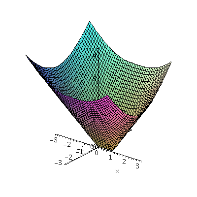
In general, continuous functions on
R2 can be much more complicated than analytic
functions. For example,
consider the function which assigns to a point (x,y) its distance to
the unit interval (the set of points (x,0) where x is between 0 and
1. Then the function is complicated. To the right is a Maple
picture of its graph. It sticks to the bottom (it is equal to 0) on
the whole interval.
f:=(x,y)->piecewise(x<0,sqrt(x^2+y^2),x<1,abs(y),sqrt((x-1)^2+y^2));
plot3d(f(x,y),x=-3..3,y=-3..3,grid=[50,50]);
If an analytic function f(z) is not the zero function (zero at
every point), then every z0 is surrounded by z's where the
function is not 0. The zeros are isoloated. That means the function
1/f(z) is defined (and analytic!) everywhere in the original domain of
f(z) except for some isolated points. The number of such isolated
points could be infinite -- look at sin(z) and then 1/sin(z). A
function which is analytic in a disc centered at z0 except
for the center is said to have an isolated singularity at
z0.
Examples
POLE
If f(z) is not the zero function, and if f(z0)=0, then
we know that f(z)=(z-z0)kh(z) for some positive
integer k, and h(z) is analytic and non-zero at z0
(therefore non-zero near z0. Then 1/f(z) has an isolated
singularity at z0, and 1/f(z) can be written
(z-z0)-k[1/h(z)]. As z-->z0,
certainly 1/h(z)-->1/h(z0). But the other factor has
modulus which -->infinity. Such a singularity is called a
pole.
The function sin(z)/z is interesting. It is certainly analytic
everywhere except at 0. So 0 is an isolated singularity. But the power
series for sin(z) centered at 0 has no constant term. We can "factor
out" z and then in sin(z)/z there is cancellation of z's top and
bottom. The result is a convergent power series (the radius of
convergence is infinity), and therefore the result is a function which
is analytic everywhere, including at 0.
Riemann's Removable Singularity Theorem
If f(z) has bounded modulus near an isolated singularity at
z0, then f(z) has a removable singularity at
z0.
Well, maybe, here is a counterexample: sin(1/x). That's certainly
bounded near 0 (by 1) and can't be extended over 0. But as several
students pointed out, sin(1/z) is not bounded near 0. If z is
iy, then sin(1/z) grows exponentially in modulus near 0. So
this function is not a counterexample.
There's a nice proof in the textbook. Please look at
it. The proof I tried to give in class uses Morera's Theorem. I looked
at g(z)=(z-z0)f(z). As z-->z0, g(z)-->0 (here is
where the boundedness of the modulus of f(z) near z0 is
used). Therefore if I define g(z0) to be 0, I have the
following: a function that is continuous in all of a disc centered at
z0 and which is known to be analytic everywhere in the disc
except possibly at its center. Now try the integral of g(z) over a
rectangle which does not have z0 inside or on its
boundary. By Cauchy's Theorem, this integral is 0. But move the
rectangle (integral always 0) so that it gets closer to
z0. The line integral is a continuous function of position
(that comes out of the ML inequality). So the value (always 0) as the
rectangle approaches z0 is its value when z0 is
on the boundary, and that must be 0. Therefore any rectangle with
z0 on the boundary has integral equal to 0. And any
rectangle with z0 inside can be written as a sum of
rectangles with z0 on the boundary, and hence these
integrals are 0 also.
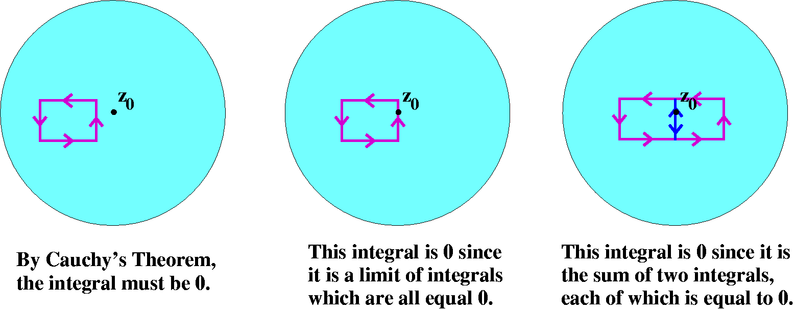
Morera's Theorem then implies
that g(z)is analytic. At z0, g(z) is zero. Therefore, the
function g(z)/(z-z0) has a removable singularity at
z0 (the argument with sin(z)/z works here). But this means
that f(z) is analytic.
Note For example, if I were told that |f(z)|>1/sqrt{|z|} for
z close to 0, it is not immediately clear (not at all!) that there is
a constant C>0 so that |f(z)|>C/|z| for z close to 0. This
occurs because the smallest that k (called the order of the
pole) could be is 1.
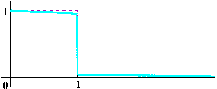
Look at f(z)=e1/z. If z is a real positive number, x, then
f(x)-->infinity as x-->0+. If z is a real negative number,
x, then f(x)-->0 as x-->0-. Therefore f(z) can be neither a
pole nor a removable singularity. Look at the graph to the right,
which displays just the f(z) for real z.
Suppose that f(z) has an isolated singularity at z0 which
is neither a pole nor a removable singularity. Then for every
w0 in C and for every a>0 and for every b>0,
there is a z with |z-z0|<a so that
|f(z)-w0|<b.
Note Sometimes this seems analogous to the idea of a black
hole in physics. When you get close to z0, f(z) gets
as close as you want to any point in C. This is an
amazing result.
Tuesday, March 29
(Lecture #17, more or less)
Please do problem 18, not problem 19, in section 2.3. Problem
19 is theoretical, but problem 18, direct computations, is more
suitable at this point in the course, I believe.
An exam problem
This one is from a written qualifying exam in mathematics given by the
University of California.
Suppose f(z) is analytic and for all positive integers k,
f({sqrt(-1)}/k}=100/k4. What is f(z) (and why)?
Well, I hope we can guess an answer. How about
f(z)=100z4. Direct evaluation shows that this function does
fulfill the given equation(s). The most important observation is that
the fourth power of i is 1! Are there any other functions? The answer
is "No," because if there were, then another function would be equal
to 100z4 on a convergent sequence, and then would have to
be indentical with this.
I discussed Mr. Radchendo's observation. I had
another motive because I needed the Bolzano-Weierstrass Theorem
below. Heh, heh, heh.
These are the contents of problem #18 of section 2.4. They follow
directly from the Cauchy integral formula for
derivatives. Use the ML estimate to get
|f(n)(z0)|<=[n!/(2Pi)]LM where L is 2Pi r
(the length of the circle of radius r centered at z0) and M
is the max of |f(w)/(w-z0)n+1| for
|w-z0|=r. This gives exactly the conclusion of problem
#18:
|f(n)(z0)|<=[n!/rn]max|z-z0|=r|f(z)|.
The |(w-z0)n+1| gives an rn+1 and the
2Pi's cancel.
Suppose someone comes up to you on the street and gives you an entire
function, f(z), with the following silly property:
|f(z)|<=4(1+|z|)10.
What can you say about f(z)?
But
|f(z)|<=4(1+|z|)10, so if |z-z0|=r, then
|f(z)|<=4(1+|z-z0+z0|)10<=4(1+|z-z0|+|z0|)10<=4(1+r+|z0|)10
if |z-z0|=r.
Combine these to get
|f(11)(z0)|<=[11!/r11]4(1+r+|z0|)10
which is true for all r>0. In particular, look at what happens as
r-->infinity. The complicated stuff has 11 powers of r on the bottom
and 10 powers of r on the top. Hey: that means
|f(11)(z0)| is overestimated by something that
-->0. Therefore |f(11)(z0)|=0 for all
z0's. Therefore f(z) must be a polynomial of degree at most 11.
I think this is from a Rutgers exam. Here the estimate given is
something like |f(z)|<=sqrt(1+|z|) for all z, and the question
again is: what can you conclude? Hey, here is a
hint and here is the answer.
We already saw this proof technique in its simplest version, Liouville's Theorem. Let me show you what I think is
the fastest proof of the Fundamental Theorem of Algebra. I did this is
class for an example. Let me try again, with a slightly different
exposition.
|(5+i)z-1|<=sqrt(6)/100
|-4z-5|<=4/(100)5
|z-6|<=1/(100)6
|-9z-7|<=9/(100)7
So now look at
|1+(5+i)z-1-4z-5+z-6-9z-7|. Use the reverse triangle inequality to
conclude that this mess has modulus at least
1-(sqrt(6)/100+4/(100)5+1/(100)6+9/(100)7)
and this is greater than, for example, 1/2.
1/p(z) will have modulus at most
2/(100)7 when |z|>100.
takes care of verifying boundedness on the outside of the disc of
radius 100 centered at 0. How about the inside?
Suppose that f(z) is 0 at z0. Look at this
sequence:
f(z0),
f´(z0),
f´´(z0),
f(3)(z0),
f(4)(z0),
f(5)(z0),
...
The sequence certainly begins with 0. Could it be all 0? Well, if it
is all zero, then f(z) must be the zero function.
Otherwise some first number in the sequence is not zero. The number of
the derivative of f which isn't 0 is called the order of the
zero of f(z) at z0.
I think I did something like this:
look at f(z)=(cos(z)-1+(1/2)z2)5. Certainly
f(0)=0. What is the order of the zero of f(z) at 0?
We could start differentiating f(z) and plugging in 0 and see
when the result is not 0. Or we could be slightly devious.
f(z)=([1-(1/2)z2+(1/24)z4+HOT]-1+(1/2)z2)5 whjere HOT stands for "higher order terms".
Then f(z) must be ([(1/24)z4+HOT])5. Now I hope
you can see easily that f(z) has a zero of order 20 at 0 and even that
the 20th derivative of f at 0 has value
(20!)/(24)5 (the 20! comes from the formula for the
coefficients of the Taylor series).
Thursday, March 24
(Lecture #16, more or less)
The diary web page was taking longer and loonger to load even with a
fast internet connection so I decided to chop it up.
I decided I should go backwards and go over some of the tougher or
more obscure things I discussed last time. So that's what I did, at
least for the first hour.
The perils of integral(sum)=sum(integral)
One thing I did last time was interchange an integral
and a sum. I wanted to spend some time on this. Indeed, we
actually counted the math symbols in the equation I wrote, and
discovered that there were 41 of them on just one side, and that's too
darn many to understand. I wanted to simplify the situation as much as
possible to show you how bad things could be. So instead of a complex
line integral, I looked at "standard" real integrals of continuous
functions on intervals of R.
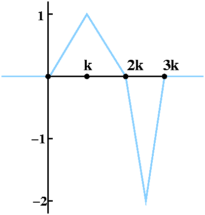 The function I began with is graphed to the right. f1(x) is
a piecewise-linear continuous function, and is not 0 only in the
interval [0,3k]. Here k will be some positive real number I don't
really care about. For x<0 and for x>3k,
f1(x)=0. Then the graph "connects the dots" (0,0), (k,1),
(2k,0), (2k+k/2,-2) and (3k,0) linearly. Certainly the integral of
f1(x) from 0 (or anything less than 0) to 3k (or anything
greater than 3k) is 0. The triangles cancel out.
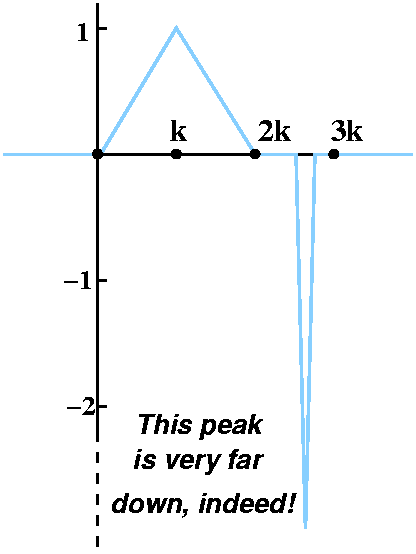
The function I began with is graphed to the right. f1(x) is
a piecewise-linear continuous function, and is not 0 only in the
interval [0,3k]. Here k will be some positive real number I don't
really care about. For x<0 and for x>3k,
f1(x)=0. Then the graph "connects the dots" (0,0), (k,1),
(2k,0), (2k+k/2,-2) and (3k,0) linearly. Certainly the integral of
f1(x) from 0 (or anything less than 0) to 3k (or anything
greater than 3k) is 0. The triangles cancel out.
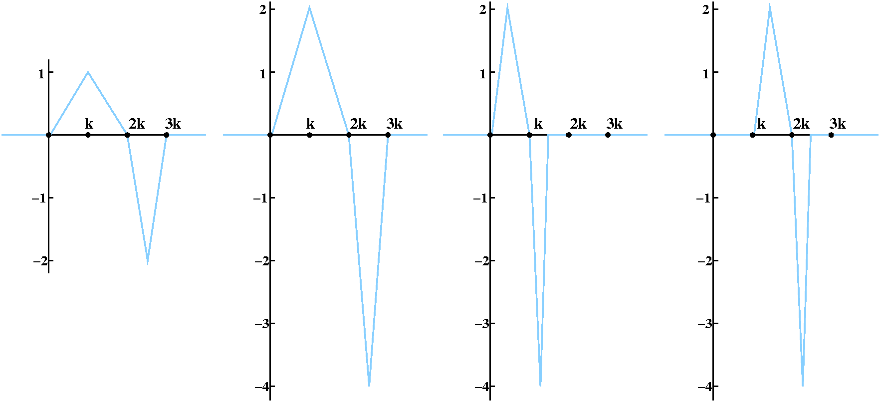
Notice please that the integral of f2(x) is again 0. Notice
that in the sum f1(x)+f2(x), the lower triangle
of f1 is canceled by the upper triangle of
f2. The sum of the two functions is 0 away from (0,3.5k).
fn+1(x)=2fn(2[x-k/2n-2])
I think this is the formula I want. fn+1 should be a
function which has one positive triangle of height 2n-1 and
width k/2n-2, and a negative triangle of height
2n and width k/2n-1. Its total integral is 0.
 What is the most interesting about this is the finite sum,
SUMn=1mf_n(x) where m is very large. It
takes some effort to see that there is lots and lots of
cancellation. The total integral is 0, this sum function "sits" inside
the interval [0,3k], and it has one "stable" positive fat triangle to
the left, and one very thin, very long negative triangle on the right.
The total integral of this is 1. Now what is
limm-->infinitySUMn=1mf_n(x)?
In fact, if you think very carefully about this, the limit is 0
except for the stable positive fat triangle. The integral of this
stable positive fat triangle is k, which isn't 0. But what about this
limit:
What is the most interesting about this is the finite sum,
SUMn=1mf_n(x) where m is very large. It
takes some effort to see that there is lots and lots of
cancellation. The total integral is 0, this sum function "sits" inside
the interval [0,3k], and it has one "stable" positive fat triangle to
the left, and one very thin, very long negative triangle on the right.
The total integral of this is 1. Now what is
limm-->infinitySUMn=1mf_n(x)?
In fact, if you think very carefully about this, the limit is 0
except for the stable positive fat triangle. The integral of this
stable positive fat triangle is k, which isn't 0. But what about this
limit:
limm-->infinity![]() 03kSUMn=1mf_n(x) dx.
03kSUMn=1mf_n(x) dx.
Each of these integrals is 0, as we've noted, so the limit exists and
is 0.
limm-->infinity![]() 03kSUMn=1mf_n(x) dx=0
and
03kSUMn=1mf_n(x) dx=0
and
![]() 03klimm-->infinitySUMn=1mf_n(x) dx=k
which is not 0.
03klimm-->infinitySUMn=1mf_n(x) dx=k
which is not 0.
So infinite sum and integral may not "commute"!
There are conditions which guarantee equality when integral and sum
are exchanged. One such condition is called uniform
convergence. I'll just outline what happens. Sometimes Math 311
covers this material, although I did not in my
last instantiation of 311.
|![]() abSUMn=1mf_n(x)-F(x) dx|<=
abSUMn=1mf_n(x)-F(x) dx|<=![]() ab|SUMn=1mf_n(x)-F(x)| dx<=(b-a)epsilon
for all m>N. This implies that
limm-->infinity
ab|SUMn=1mf_n(x)-F(x)| dx<=(b-a)epsilon
for all m>N. This implies that
limm-->infinity![]() abSUMn=1mf_n(x) dx=
abSUMn=1mf_n(x) dx=![]() abF(x) dx.
abF(x) dx.
If you are clever, you can see that we're using a version of the ML
inequality to prove this. So uniform convergence imples that So
infinite sum and integral do "commute" if uniform convergence
is also assumed.
We compared power series
inside their radius of convergence to a fixed convergence
geometric series. We were really proving that in any subdisc which is
strictly contained inside the radius of convergence, the power series
converges uniformly. So we can actually interchange sum and integral.
I asserted last time that, given any x0 in R,
1/(1+x2) had a power series expansion centered at
x0 with radius of convergence at least 1. This is true but
is certainly not obvious. How can I produce the power series expansion
for you? I could try to differentiate the function and create a Taylor
series. I think Maple does this:series(1/(1+x^2),x=5,5);
1 5 37 30 719
-- - ---*(x-5) + ----*(x-5)^2 - -----*(x-5)^3 + -------(x-5)^4 + O((x-5)^5)
26 338 8788 28561 2970344
This is too hard for me. There's another way which we will exploit
systematically later.
(i/2)/([x-5]+[5-i])={-(i/2)/(i-5)}{1/[1-(-r)]}={-(i/2)/(i-5)}SUMn=0infinity(-1)n[(x-5)/(5-i)]n=(i/2)SUMn=0infinity[(-1)n/(5-i)n+1](x-5)n.
So we have a piece of the power series. We can do something analogous
with the other piece, (i/2)/(x+i). We will get
(i/2)SUMn=0infinity[(-1)n+1/(5-i)n+1](x-5)n,
I think.
 If you add up the two pieces, you'll get the total power series for
1/(1+x2) centered at x0=5. What's the radius of
convergence of this series? We need r=(x-5)/(5-i) to have modulus
less than 1. When does this occur? The modulus of 5-i is sqrt{26}. So
actually the radius of convergence is sqrt{26}, and why is this?
If you add up the two pieces, you'll get the total power series for
1/(1+x2) centered at x0=5. What's the radius of
convergence of this series? We need r=(x-5)/(5-i) to have modulus
less than 1. When does this occur? The modulus of 5-i is sqrt{26}. So
actually the radius of convergence is sqrt{26}, and why is this?
Complex results usually turn out to be much simpler. Therefore if you
can turn a real problem into a complex problem, it is likely that the
problem will be simpler. Probably. Maybe. Anyway, that's what many
people think.
We took a ten-minute break. Snacks were served.
The textbook and class lectures have given two or three ways of
defining a function which should be sin(z). That is, we would like an
entire function, that is, a function analytic on all of C, which when
restricted to R is the standard sine function. How many candidates
are there for such a function, and how would we identify such
candidates.
Well, if I look at the standard sin(x) function defined in calculus,
then I know that sin(0)=0, sin´(0)=1, sin´´(0)=0,
sin´´´(0)=-1, and then the values begin to cycle. If
there is an entire function which should be sine, then, as we saw last
time, that function should have a power series centered at 0 (actually
the series could be centered at any point!) whose radius of
convergence is infinity. But now plug in the numbers, and get the
complex power series
SUMn=1infinity[(-1)n/(2n+1)!]z2n+1.
This is the only power series centered at 0 which has the correct
derivatives. Therefore the function defined by this series (whose
radius of convergence is infinity!) must be sine, and is sin(z).
We can generalize this result.
IF
f(z) and g(z) are analytic in a domain D, and if there is a point
z0 in D so that the values of f and g and all their
derivatives agree at z0
THEN
f(z)=g(z) in all of D.
 A proof of essentially this result is on p.127 of the text. How does
the proof go? First, because the function values and all the
derivatives agree at z0, the power series at z0
for f(z) and g(z), which are Taylor series for z0,
must be the same. Therefore, the functions f(z) and g(z), which are
equal in a disc to the sum of these series, must agree. But then we
want to extend the agreement to all of the domain. Remember that
domains are connected open sets. So connect z0 with
any other point by a curve inside the domain. Use that curve to draw a
chain of discs each of which has its center inside the disc
before it. Then inductively, f(z)=g(z) on one disc, so all the
derivatives are equal so that the power series for each function at
the next center will be equal, making f(z)=g(z) on that disc, etc.
A proof of essentially this result is on p.127 of the text. How does
the proof go? First, because the function values and all the
derivatives agree at z0, the power series at z0
for f(z) and g(z), which are Taylor series for z0,
must be the same. Therefore, the functions f(z) and g(z), which are
equal in a disc to the sum of these series, must agree. But then we
want to extend the agreement to all of the domain. Remember that
domains are connected open sets. So connect z0 with
any other point by a curve inside the domain. Use that curve to draw a
chain of discs each of which has its center inside the disc
before it. Then inductively, f(z)=g(z) on one disc, so all the
derivatives are equal so that the power series for each function at
the next center will be equal, making f(z)=g(z) on that disc, etc.
Sometimes I think that analytic functions are just infinite degree
polynomials. And sometimes the analytic functions agree with me (?)
and behave well. One way we could get two polynomials to be equal
everywhere is to get them to agree at sufficiently many points. For
example, if P(x) and Q(x) are polynomials on R, of degree, say, at
most 14, and if the set where P(x)=Q(x) has at least 15 points, then
P(x) and Q(x) must be the same polynomials everywhere. This sort of
implication is used everywhere in numerical analysis, but is probably
easiest to see using linear algebra. Notice that P(x) and Q(x) have 15
parameters (their coefficients) and making them agree at 15 points
gives 15 linear equations in these parameters. The coefficient matrix
involved in this system of linear equations is a Vandermonde
matrix which has a non-zero
determinant.
Suppose I know that f(z) is an entire function and, for example, I
also know that f(1/2k) is equal to
sin(1/2k). Then, in fact, f(z) must be sin(z), and,
certainly, for all real x, f(x)=sin(x).
This is a remarkable result.
Why is it true? Well, since sin(x) is continuous,
sin(0)=limk-->infinitysin(1/2k). But this is
the same, since f(z) is continuous and the numbers inside the
limit agree, as
f(0)=limk-->infinitysin(1/2k).
But ... but ... maybe it would be better to prove this in general.
IF
f(z) and g(z) are analytic in a domain D, and there is a sequence
{zk} with f(zk)=g(zk) for all k and,
finally, limk-->infinityzk=z0, a
point in D,
THEN
f(z)=g(z) in all of D.
Both f and g are analytic so they are continuous. Therefore since we
know that limk-->infinityzk=z0,
we see limk-->infinityf(zk)=f(z0),
and
limk-->infinityg(zk)=g(z0).
But f(zk)=g(zk) for all k, so
f(z0)=g(z0).
Look at the power series for f centered at z0:
f(z)=SUMn=0infinityan(z-z0)n. And
look at the power series for g centered at z0:
g(z)=SUMn=0infinityan(z-z0)n.
Remember that each series is a Taylor series. Since
f(z0)=g(z0), a0=b0. Now
consider the functions ff(z)=[{f(z)-a0}/(z-z0)]
and gg(z)=[{g(z)-b0}/(z-z0)]. Although we seem
to be dividing by z-z0 and therefore making trouble, in
fact, the series for f(z)-a0 and the series for
g(z)-b0 both have common factors of z-z0, so we
are just canceling just common factors, non-zero away from
z0. The results are convergent power series and therefore
are analytic functions.
The functions ff and gg agree at
each of the complex numbers zk. Therefore, just as in the
previous argument, ff(z0)=gg(z0), and that means
a1=b1.
Let us write two new functions:
fff(z)=[{f(z)-a0-a1(z-z0)}/(z-z0)2]
and
ggg(z)=[{g(z)-b0-b1(z-z0)}/(z-z0)2].
These functions are also analytic, because although we are dividing by
(z-z0)2 we have taken away the only parts of the
power series where this would be an obstable. Also I know that
fff(zk)=ggg(zk) since
f(zk)=g(zk) and a0=b0 and
a1=b1. Whew. Just as twice before, we now
conclude that fff(z0)=ggg(z0), and that means
a2=b2.
Well, why is the instructor so stubborn that he won't give a proof
using mathematical induction? Well, it will work and we will get
all of the coefficients of the power series for f and g
centered at z0 to agree, and therefore f(z)=g(z) in
all of the domain.
Well look at f(z)=sin(x)cosh(y)+icos(x)sinh(y). This function is
analytic because it satisfies the Cauchy-Riemann equations. But notice
that since cosh(0)=1 and sinh(y)=0, f(x+i0)=sin(x) for all real x.
Hey, that certainly satisfies the hypotheses of the result we've just
proved. So f(z) must be sin(z) for all complex z!
This result was proved with the help of Cohen2: why does
(sin(z))2+(cos(z))2=1? Both sides of this
equation are entire functions. The equality is true on all of the real
numbers. Therefore, since the real numbers have a convergent sequence
(!!), the equality is true for all of C.
Both of the results we've proved are at the beginning of what's called
analytic continuation. We take functions and equations that
work on a small set, and then, "automatically", things will work on a
larger set. This is weird, remarkable, and useful.
I'll mention this next time, but look: Mr. Radchenko declared that
although having f(z)=g(z) at an infinite number of z's isn't enough to
guarantee that f(z) must equal g(z) everywhere (cosine and sine!), if
we ask that f(z)=g(z) at an infinite number of z's which are bounded,
then they must be equal.
Why is this? Because (and this is a result from advanced calculus):
There's a proof using "bisection" in my 311 diary for
3/12/2003. Sigh. Look at 311,
please. Bolzano-Weierstrass
Theorem Suppose (xn) is a sequence all of whose terms
are in [a,b]. Then (xn) has a convergent
subsequence.
If you are willing to believe this result, then you get a sequence
where f(z)=g(z) which has a limit point, and ... you're done!
Tuesday, March 22
(Lecture #15)
We saw that the sum of a power series was analytic, and that the
derivative of this sum is equal to the sum of the terms of the series
differentiated: that is, a convergent power series behaves very much
like we'd believe an "infinite" polynomial to behave.
We started with an analytic function defined in a simply
connected domain. (One way of recognizing such: "No holes.") Then
the integral of the analytic function around any simple closed curve
is 0. I proved this with Green's Theorem, and I needed to assume that
the analytic function had a continuous derivative. That turns out not
to be necessary ("Goursat") but right now I don't care!
Suppose that a path in a simply connected domain is closed and is made
up of a finite number of horizontal and vertical line segments. Then
the integral of an analytic function around this path is 0.
Suppose we have a continuous function defined in a domain, and we know
that the integral of this function around a rectangle whose interior
is in the domain is 0. Then the function has a primitive: that is, the
function is the derivative of an analytic function. (Here we
"constructed" the primitive by a process resembling what's done in
physics and third semester calculus to get a potential from a
conservative vector field.)
This result, which I will abbreviate as CIF, is really weird. If you
have a function f(z) that's analytic on and inside a simple closed
curve, C, and if z is inside the curve, then
f(z)=[1/(2Pi i)]![]() C[f(w)/(w-z)]dw.
C[f(w)/(w-z)]dw.
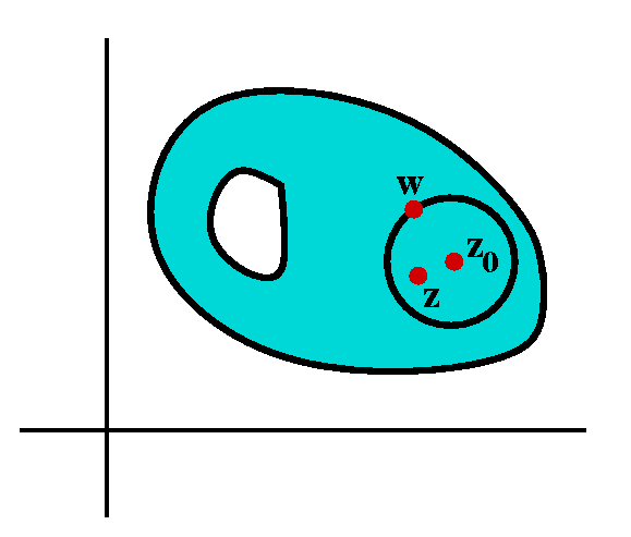 This title refers to a really remarkable process which, even though it
is 170 years old, is still interesting to me. We use it to get much
information from the CIF. The Cauchy kernel is 1/(w-z). Here is
the setup:
This title refers to a really remarkable process which, even though it
is 170 years old, is still interesting to me. We use it to get much
information from the CIF. The Cauchy kernel is 1/(w-z). Here is
the setup:
f(z) is analytic in a domain D. We select z0 in D. We
select a positive radius r so that the circle of radius r centered at
z0 and its inside are contained entirely within D. Also
take any z inside the circle. Then the CIF implies that
f(z)=[1/(2Pi i)]![]() |w-z0|=r[f(w)/(w-z)]dw.
|w-z0|=r[f(w)/(w-z)]dw.
Let's look at 1/(w-z), where w is on the circle. Then, as I showed in
class, and is clearly written in the text, we write:
1/(w-z)=1/(w -z)=1/(w - + -z)=1/(w-z0+z0-z).
This sort of thing is all routine now, but please try to imagine the
excitement of inventing (discovering?) it. Now also realize
that for w on the circle, |w-z0|=r and since z is
insided the circle, |w-z|<r. Now we need other neurons to
"fire" and some synapses to connect. Well,
|(w-z)/(w-z0|<1. And so
1/(w-z0+z0-z)=[1/(w-z0)][1/(1-s)]
where s=[(w-z)/(w-z0)] is a complex number whose modulus
is less than 1. So we can use the geometric series, which I have
mentioned again and again is almost the only series we really need to
know.
I interchanged the sum (which resulted from e-x-p-a-n-d-i-n-g the
Cauchy kernel) and the integral. I remarked that this was a
mathematically perilous step and I will go into this more in the next
class. In this case, with a geometric series, we can make very explicit
error estimates, comparing partial sums and the various infinite tails
of the series. This is done in the text and students should at least
look at the material.
f(z)=SUMn=0infinityan(z-z0)n,
where the an's are coefficients and magically given by the
formula
an=[1/(2Pi i)]![]() |w-z0|=r[f(w)/(w-z)n+1]dw.
|w-z0|=r[f(w)/(w-z)n+1]dw.
Apparently we just proved that an analytic function must have a power
series expansion which is valid in any disc contained in its
domain. Let's see: since we can differentiate power series any number
of times. Therefore we have proved:
The derivative of an analytic function is analytic.
So one derivative implies many, many more!
Certainly in calculus this is false, since there are many
functions which give non-differentiable results when you differentiate
them.
Also please realize that we already know that a power series for a
function must be the Taylor series (we did this is lecture #12, on
March 1). Therefore the an's must be
[f(n)(z0)]/n!, and we have proved what is
usually called
The Cauchy Integral Formula for Derivatives
f(n)(z0)=[n!/(2Pi i)]![]() |w-z0|=r[f(w)/(w-z)n+1]dw.
|w-z0|=r[f(w)/(w-z)n+1]dw.
Here is a totally silly result. I know of no application of this
result.
IF
you have a function f(z)
defined on all of the complex numbers (all of C) with the
following ludicrous property:
For any point z0 in the plane, f(z) is equal to the sum of
a power series centered at z0, and this power series has
radius of convergence equal to 1.
THEN the radius of convergence of f(z)'s Taylor series centered
at any point is infinite, and f(z) is equal to the sum of that
power series.
Since f(z) is a sum of a power series near every point, f(z) is analytic
in all of C. Since f(z) is analytic in all of C,
then I can take the r in the picture/proof above as big as I like and
the darn series will have infinite radius of convergence. So I'm done!
Below is a suitably silly picture illustrating this "result" (?).
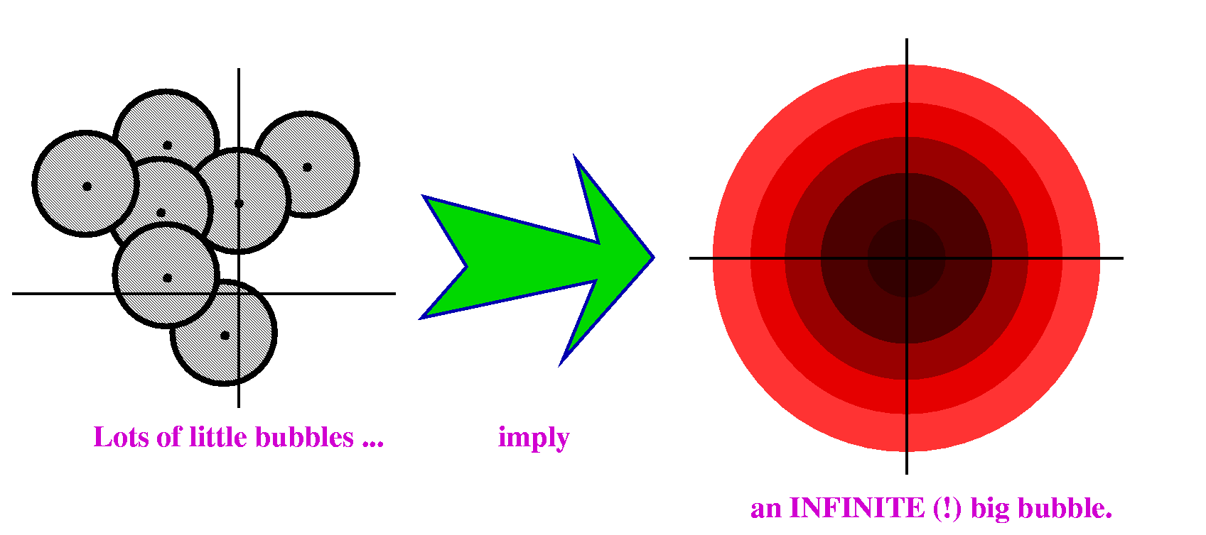
(At least for R!) I claimed that 1/(1+x2) was a
function which was equal to a power series valid in some interval
around every point. I will talk more about this in the next class.
Suppose I have a continuous function f(z) in a domain, and I know that
for any rectangle whose inside is contained in the domain, the
integral of f(z) around the boundary of the rectangle is 0. Well, if
you look back, you can see that this condition
implies that f(z) has an analytic primitive or antiderivative: there
is an analytic function F(z) whose derivative is f(z). But ... but
... the derivative of an analytic function is analytic. We have just
proved
Morera's Theorem: If f(z) is a continuous function and and if the
integral of f(z) around the boundary of any rectangle whose
inside is contained in the domain is 0, then f(z) is
analytic.
This is nice because integrals are usually much easier to handle than
derivatives. Integrals are averages, and derivatives are quotients of
tiny numbers, so derivatives are more unstable than integrals almost
by their nature. Weird, weird ...
There are almost surely no more major proof techniques to be shown in
this course. The bag of tricks is empty. Of course, we will use the
techniques in many different specific applications. But ... we have
obtained a wonderful result:
The following characterizations of a function are logically
equivalent:
ux=vy
uy=-vx
An entire function f(z) (analytic in all of C) which is
bounded (so there is a [positive] real constant M with
|f(z)|<=M for all z) must be constant.
Yet another counterexample (?)
sin(x)? Well, not really. sin(z) if z=iy is actually
isinh(y). So sin(z) grows exponentially along the imaginary
axis.
I proved this by looking at f´(z) with the CIF for derivatives and
showing (via ML) that this must be 0. The proof is in the text.
I will lecture from 6:10 to 7:10, take a 10 minute break, and then
lecture for another hour. I would like to do this for the next few
Thursdays and catch up with the other section.
Please hand in these problems on Thursday, March 24:
2.3: 1, 2, 4, 9, 10, 14.
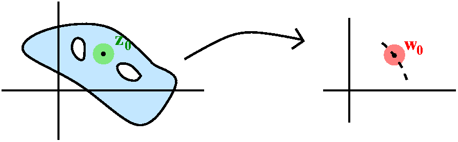
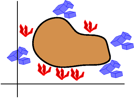 A very dilute bit of physics
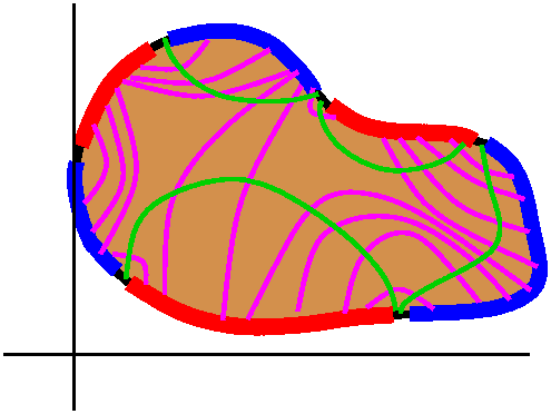 Suppose I give you a heat distribution on the edge of the plate, as
shown. The red stuff is supposed to be flames, and the blue stuff is
supposed to be ice cubes. If I let time "flow" and keep the ice cubes
and flames on the edge, maybe you can see that eventually the
temperature distribution inside the plate will stabilize, and we will
get a steady state temperature distribution. Maybe you can see the
flow curves ("flux") and the isothermals. These curves are the level
lines of harmonic functions. There are no closed curves, because
otherwise the minimum/maximum principles would be violated.
The curves are perpendicular to each other because they represent
curves on which an analytic function has fixed real and imaginary
values, and the real and imaginary axes are perpendicular, and
analytic functions are generally conformal.
Suppose I give you a heat distribution on the edge of the plate, as
shown. The red stuff is supposed to be flames, and the blue stuff is
supposed to be ice cubes. If I let time "flow" and keep the ice cubes
and flames on the edge, maybe you can see that eventually the
temperature distribution inside the plate will stabilize, and we will
get a steady state temperature distribution. Maybe you can see the
flow curves ("flux") and the isothermals. These curves are the level
lines of harmonic functions. There are no closed curves, because
otherwise the minimum/maximum principles would be violated.
The curves are perpendicular to each other because they represent
curves on which an analytic function has fixed real and imaginary
values, and the real and imaginary axes are perpendicular, and
analytic functions are generally conformal.