We could think that the region inside the uv circle is broken up into
many small pieces of area dAuv and then these are magically
(?) transported to the xy plane, and they form the interior of an
ellipse with horizontal semimajor axis of length 2 and vertical
semiminor axis of length 1. What is the area inside the ellipse? Here
is one way to compute that area:
Area of xy ellipse=∫∫ellipse in
xy1 dAxy=∫∫circle in uv1 (2dAuv)=2∫∫circle in uv1 dAuv=2(π12).
The justifications for each of these equalities is much the same as
what was written above. Basically, small chunks of area get stretched
by 3 and the result gets stretched by 3.
Please notice that these are relatively simple stretchings and area
multiplications. In more complicated situations, the area stretching
will change from at different points. (Actually, exactly that happens
with, say, polar coordinates. There is non-uniform stretching, the
multiplication by r, which occurs.)
I used scaling=constrained because if that's removed, some of the
effect of the shear seems to be undone. Try it, and see what you get
(a tilted ellipse with y=x as one axis, actually, and then you should
explain this!).
Since 1dAuv=dAxy, the total area is not
changed at all. Therefore the area inside
x2-10xy+26y2=1 is exactly equal to
π12. I think if I worked diligently with dxdy
integrals and used trig substitutions as they are taught in 152 I
might, after a while, be able to get this result. But a whole
heck of a lot of work would need to be done.
So what's going on ...
This result is not used as in the past examples. That is, people don't
decide, "Hey, let's look at u and v and see ..." Rather, what happens
is that sometimes folks realize they need to evaluate some (horrible)
double/triple/whatever integral. They look at it, and see, somehow,
some sort of links between the integrand and the region. They see,
somehow, that everything could be described in terms of other
variables. Then they reach in and use the result that follows. Note
that no one I know uses this result "casually" -- they use it only if
they really need it.
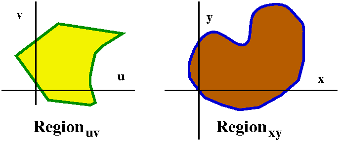 The theorem
Suppose x and y are written as functions of u and v. Then JAC, the area distortion factor, is the absolute
value of a certain determinant:
    | ∂x/∂u ∂x/∂v |
det |             |
    | ∂y/∂u ∂y/∂v |
If Ruv is a region in the uv plane and Rxy is
the corresponding region in the xy plane, if FUNCxy is a function written in terms
of x and y, and if FUNCuv is the function rewritten
in terms of u and v, then
∫∫RuvFUNCuv (JAC) dAuv=∫∫RxyFUNCxydAxy
Names
JAC is called the Jacobian. The
result above, discussed in section 15.4, and particularly stated on
pages 928 and 929 of the text, is called the Change of Variables
Formula.
So ...
This theorem is difficult to work with but wonderful when you can use
it. Here are two computations I showed in class.
This example is artificial but useful as a start
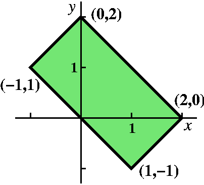 Compute
∫∫R(x-y)40(x+y)50dA where R is
the rectangular region with corners (1,-1), (2,0), (0,2), and (-1,1).
This is an irritating integral. But there is some not well concealed
symmetry. The boundaries of rectangle can be written as x+y=2,
x+y=0, x-y=-2, and x-y=2.
It almost seems as if the integrand and the region are begging
us to rewrite everything in terms of u and v where u=x-y and
v=x+y. Then the region of integration can be described -2<=u<=2
and 0<=v<=2. The integrand becomes
u40v50. Notice that if we add the equations
u=x-y and v=x+y and divide by 2 we get x=(1/2)(u+v). If we subtract
the first equation from the second and divide by 2 we get
y=(1/2)(v-u).
What's JAC?
Since x=(1/2)(u+v) and y=(1/2)(v-u) we compute
    | ∂x/∂u ∂x/∂v |       | 1/2  1/2 |
det |             | = det |          | = -1/4 -1/4 = -1/2
    | ∂y/∂u ∂y/∂v |       | 1/2 -1/2 |
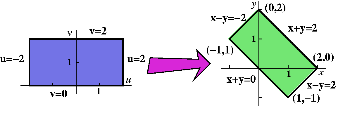 JAC is the absolute value, 1/2.
We have in effect parameterized the xy plane with
(1/2)(u+v)=x and (1/2)(v-u)=y. So everything in x and y could be
written in terms of u and v. The "General Change of Variables"
result becomes what follows in this case:
∫∫Rxy(x-y)40(x+y)50dAxy=∫v=0v=1∫u=-2u=2u40v50(1/2)du dv.
This can be evaluated exactly easily because it is just a mess of
powers of u and v. The answer is:
(1/2)2·(241/41)(251/51).
Crazy people all over ...
Or you could just try it in Maple as it
is. But we will need to break up the integral into three pieces (in
either dxdy or dydx). Also, I want to learn how much time and space
the computation takes, so I will use showtime.
The instruction showtime(true); has this
effect (from the Help page):
Any Maple statement entered is evaluated normally, its result returned
followed by a line numbered O1, O2, .. with the time taken and the
amount of memory used being displayed.
Here we go.> showtime(true);
O1 := func:=(x-y)^40*(x+y)^50;
40 50
(x - y) (x + y)
time = 0.00, bytes = 7382
O2 := A:=int(int(func,x=-y..2+y),y=-1..0);
618970019642690137449562112
---------------------------
1173
time = 0.08, bytes = 1394659
O3 := B:=int(int(func,x=-y..2-y),y=0..1);
41125671617232447642991204624847361028540479941115904
-----------------------------------------------------
62654905899056975234831847747
time = 0.08, bytes = 1275540
O4 := C:=int(int(func,x=-2+y..2-y),y=1..2);
74187486054615395748140995710384329611242731900764160
-----------------------------------------------------
62654905899056975234831847747
time = 0.13, bytes = 1880463
O5 := A+B+C;
4951760157141521099596496896
----------------------------
2091
time = 0.00, bytes = 3963
O6 := %-(2^(41)*2^(51))/(41*51);
0
time = 0.00, bytes = 3988
So our result is the same as the rather painful direct computation,
which took a total of .29 seconds. That is not terrible, but that
computation gave no insight, which is bad.
|
What's going on?
If there is something common among the algebraic and geometric
specifications of a double (or a triple!) integral, then we can
sometimes take advantage. That's what's going on.
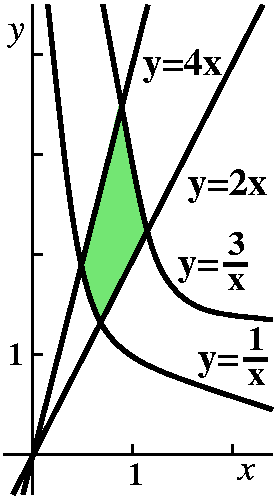 Another example, but this one more realistic
The following example could arise in thermodynamics or physical
chemistry. Suppose R is the region in the first quadrant bounded by
y=2x, y=4x, y=1/x, and y=3/x. Let's compute ∫∫Rx4y dA.
Here a neat "change of variables" is a bit hidden, but maybe you can
see that the boundary curves of the region are y/x=2 and y/x=4 and
xy=1 and xy=3. Then you might (!) think to define u=y/x and v=xy. If
you do, then uv=(y/x)(xy)=y2 so that
y=u1/2v1/2. Then v=xy becomes
v=x(u1/2v1/2) so that
x=u-1/2v1/2. With the equations
x=u-1/2v1/2 and y=u1/2v1/2
the original integrand
x4y becomes u-3/2v5/2. The Jacobian
computation is:
      | ∂x/∂u ∂y/∂u |       | -(1/2)u-3/2v1/2 (1/2)u-1/2v1/2 |
det = |             | = det |                              |
      | ∂x/∂v ∂y/∂v |       | (1/2)u-1/2v-1/2 (1/2)u1/2v-1/2 |
and this is -(1/4)u-1-(1/4)u-1. We want the
absolute value so we have (1/2)(1/u). In this case, which is
considerably more complicated than the others above, the amount of
stretching sepends on the value of u. In the other cases we looked at
previously, the stretching was the same at all points. In the real
world, non-uniform stretching is more likely. (Take either a piece of
taffy or a steel bar and pull at the ends. I bet that the parts near
the ends stretches more than the center.) The double integral which
results is
∫13∫24u-3/2v5/2(1/2)(1/u)du dv.
The region of integration has become a rectangle, the integrand is not
horrible, and the Jacobian factor is also not too bad. I won't
compute this, but I hope that you see it is easy enough.
Polar and spherical ...
The factors involved in integration in polar/cylindrical
(r drd&theta) and spherical
(ρ2sin(φ) dρdφdθ) all come
from Jacobian calculations. The spherical factor is the absolute value
of a determinant of a 3-by-3 matrix. The computation is not fun. I've
done it several times and have managed to make mistakes each time.
Proof? Who needs a proof?
Verification of the change of variables formula for double and on up
integrals is very difficult. What's needed is knowledge of linear
algebra and lots of comfort with limit processes, since the two sides
of the formula are quite complicated Riemann sums. Working through the
proof in detail takes about two weeks in an upper-level math
course. Please believe this result, and try a few examples on your
own.
Ms. Jain's request
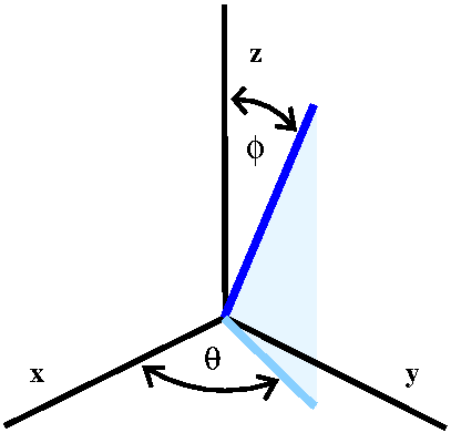 The planes x=0 and y=0 and z=0 divide R3 into eight
chunks. Differently put, if you remove these planes from space, you'll have
eight pieces left. Each of the eight pieces is characterized by
requiring that the variables x, y, and z have specific (non-zero!)
signs. Ms. Jain asked how the spherical
coordinates φ and θ relate to these sign restrictions.
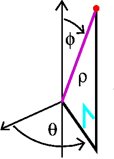
Look to the right. There is a very bare diagram with the spherical
angles φ and θ sketched. Of course, φ is the angle
between the radius vector and the positive z-axis. People usually
request that φ be in the interval [0,π]. If this angle is
acute, so 0<φ<π/2, then the radius vector will be
above the xy-plane, no matter what the value of θ. This
means z>0 exactly coincides with 0<φ<π/2. If we push
the radius vector below the xy plane, then z<0 and φ
will be larger than π/2. So z<0 is the same as
π/2<φ<π.
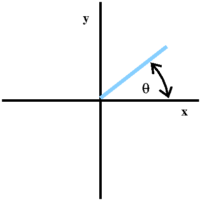 θ does not affect the sign of z at all. It interacts with the
signs of x and y. So we can just look "downwards" in R3
from high up on the positive z axis. Then we might understand what
we're seeing as something like usual polar coordinates (remember, the
z information is carried by φ so we don't need that here).
Certainly we can just read off the sign combinations of x and y by the
usual quadrant information of θ.
| Sign of x | Sign of y | Sign of z |
Interval of θ | Interval of φ |
|---|
| x>0 | y>0 | z>0 | 0<θ<Pi/2 | 0<φ<&pi/2 |
| x<0 | y>0 | π/2<θ<π |
| x<0 | y<0 | π/2<θ<3π/2 |
| x>0 | y<0 | 3π/2<θ<2π |
| x>0 | y>0 | z<0 | 0<θ<Pi/2 | π/2<φ<π |
| x<0 | y>0 | π/2<θ<π |
| x<0 | y<0 | π/2<θ<3π/2 |
| x>0 | y<0 | 3π/2<θ<2π |
I hope this is helpful to other people who are trying to understand
spherical coordinates.
|
Monday, November 3
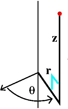 Cylindrical coordinates
This is a coordinate system that augments the r and θ of polar
coordinates with z. Any problem with an axis of symmetry may be easier
to understand in cylindrical coordinates. In words, the position of a
point in the cylindrical coordinate system is described by its height,
z, from the base coordinate plane. The foot of a perpendicular from
the point to the plane then has a description in terms of an angle,
θ, from an initial ray (usually the positive x-axis) and a
distance, r, from the origin.
Here are some basic axially symmetric figures:
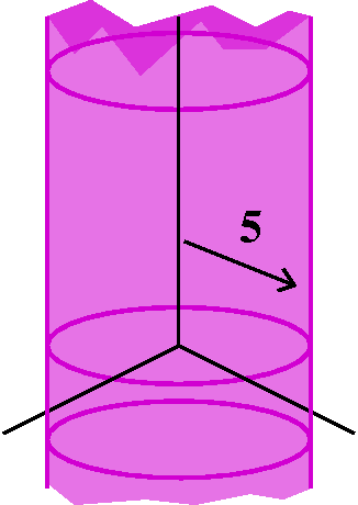
Cylinder Example: r=5.
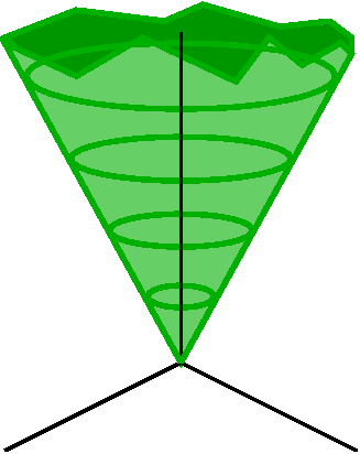
Cone Example: z=7r.
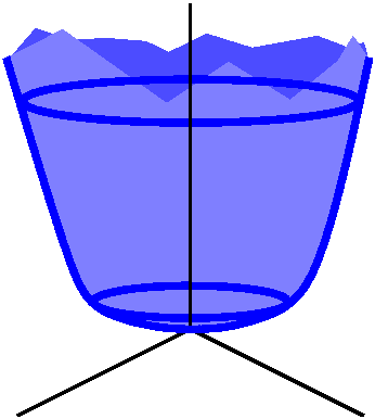
Elliptical paraboloid Example: z=3r2.
Some basic axially symmetric surfaces
|
r=5 is the collection of points in R3 whose distance
to the "axis" is 5. The axis is the z-axis, so this will be a right
circular cylinder of radius 5 having the z-axis as axis of symmetry.
|
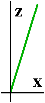 z=7r gives a right circular cone whose axis of symmetry is the
z-axis. How can you "see" this? Well, if we restrict ourselves to the
slice of this surface through the xz-plane (with y=0) we get a picture
sort of like what is shown. Why? Because if
y=0, r=sqrt(x2+y2)=x (at least for x>0), so
the result is the line shown.
In general, since θ is not restricted, we get all the points
shown as we revolve the "profile" curve around the z-axis. And this is
a cone with vertex at the origin.
|
z=3r2 is a paraboloid, because
r2=x2+y2 and you should see, I hope,
that the result is what happens when the profile curve, a parabola
through the origin, is revolved around the z-axis.
|
 |
 |
 |
The location of Frelinghuysen
Hall
I enlightened students with
these facts:
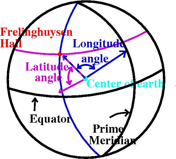 FH's latitude is 40.50411oN
and FH's longitude is 74.44836oW.
Or, in more antique fashion
(degrees/minutes/seconds), the latitude is
40o39´55.636´´ and the longitude is
74o27´5.452´´
Do not be as confused as I am. This is
not about stalactites (the down-dropping things) and stalagmites (the
up-growing things).
We discussed what latitude and longitude are. The prime meridian is a
great circle (a circle whose center is the center of the earth) and it
goes through Greenwich, England and the north/south poles. The
longitude is the angle between that great circle and the great circle
connecting FH and the north/south poles. The angle has vertex at the
center of the earth. W=west in the latitude, and it means the the
angle opens to the west of the prime meridian. Latitude is the angle
from the intersection of the great circle describing FH's longitude
with the plane of the equator, again with the vertex at the center of
the earth. N=north means that we look in the northern
hemisphere. Constant latitude means a "small" circle. Constant
longitude means a great circle (actually semicircle). FH is located at
the unique intersection on the surface of the earth of these two
curves.
I presume you know that the "23 and a half"
degree tilt of the axes (north/south pole line) from the ecliptic (the
plane of the earth's orbit about the sun) is responsible for seasonal
variation. Nature is terrific!
Spherical coordinates
Take a point in space. We describe its position with one length and
two angles. The length is the distance of the point to the origin: the
length of the radius vector. The first angle, φ, is the angle from
the positive z-axis to the radius vector. The second angle, θ, is
the angle from the positive x-axis to the projection of the radius
vector on the xy-plane. Spherical coordinates are very useful in
problems with central symmetry.
Spherical coordinates
Take a point in space. We describe its position with one length and
two angles. The length is the distance of the point to the origin: the
length of the radius vector. The first angle, φ, is the angle from
the positive z-axis to the radius vector. The second angle, θ, is
the angle from the positive x-axis to the projection of the radius
vector on the xy-plane. Spherical coordinates are very useful in
problems with central symmetry. I'll work a bit with them next
time.
I deduced the following formulas (with errors but they were
corrected):
x=ρ sin(φ)cos(θ)
y=ρ sin(φ)sin(θ)
z=ρ cos(φ)
I remarked that it was useful to know that such formulas existed, but
that I had rarely used them. One result that I have used frequently
comes from the fact that ρ represents the distance from (x,y,z) to
the origin.
x2+y2+z2=ρ2.
Standard restrictions on spherical coordinates
Because the angles sort of fold over when π's and 2π's are added,
most people who use spherical coordinates put some restrictions on how
big/small θ and φ can be. If we only allow θ to be between 0
and 2π and only allow φ to be between 0 and π, then there will be
unique spherical coordinates for every point in R3. So I
will generally work with these restrictions.
Some shapes in spherical coordinates
|
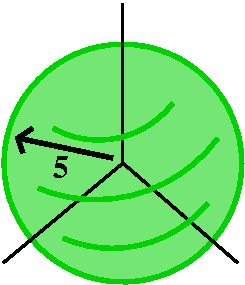
ρ=constant gives a sphere centered at the origin. So, for example,
ρ=5 is a sphere centered at the origin of radius 5.
|
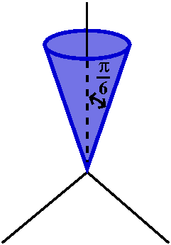
φ=constant gives a right circular cone whose axis of symmetry is the
z-axis. For example, φ=π/6 is a cone with vertex at the origin and
whose axis of symmetry is the positive z-axis. The angle between the
positive z-axis and any of the cone's "generators" (lines from the
vertex on the surface of the cone) iw π/6 (yes, 30o). The
bottom half of the cone is not included because that is where φ is
between π/2 and π.
|
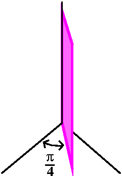
θ=constant gives a half-plane, with the z-axis being the edge of
the half-plane. For example, θ=π/4 gives a half-plane which is
perpendicular to the half-line y=x (x>0) in the xy-plane. The other
half of the plane is where θ is 3π/2, and so it is not included
in this object.
|
 |
 |
 |
Integral #1
A spherical region of radius R is filled with material whose density
is directly proportional to the distance from the origin. What is its
mass?
This is not very realistic. The center is light and
fluffy and the outer edge is heavy and tough (my kind of
cooking?). The density is supposed to interpolate linearly between
these extremes. Maybe the appropriate assignment would be to build an
object of this type.
The math setup
Take a small piece of volume, dV, in the sphere. The corresponding
piece of mass, dm, is related to dV by dm=(density)dV. We know that
the "density is directly proportional to the distance from the
origin." Place the origin of the coordinate system at the center of
the sphere. So there is some constant C>0 so
density=C ρ. And the total mass is the sum of the dm's. This
"sum" should be a triple integral:
Total mass=∫∫∫The whole ballC ρ dV.
In spherical coordinates, a description of a sphere of radius R
centered at the origin is easy: ρ goes from 0 to R, θ goes from
0 to 2π, and φ goes from 0 to π. We just use the agreed upon
ranges for the angles to sweep out a whole sphere. There is one sticky
point, however.
dV in spherical coordinates
We need to convert dV to spherical coordinates. In fact,
dV=ρ2sin(φ)dρdθdφ
I know this is true. First, there is a discussion which is supposed to
be convincing in the text (on pages 915 and 916). Second, I said it in
class. Third, I actually can give an understandable argument if there
is enough time later in the course. This strange multiplier is an
example of what is called the Jacobian, a
factor used to convert volume in one coordinate system to another. I
may have time to discuss the computation later. In
any case, when I use spherical coordinates, I almost never bother
thinking about this weird mess, but I just write it.
The computation
So we have
Total mass=∫φ=0φ=π∫θ=0θ=2π∫ρ=0ρ=R(C ρ)ρ2sin(φ)dρdθdφ.
The inner integral
∫ρ=0ρ=R(C ρ)ρ2sin(φ)dρ=∫ρ=0ρ=RCρ3sin(φ)dρ=Csin(φ)ρ4/4]ρ=0ρ=R=Csin(φ)R4/4.
The middle integral
∫θ=0θ=2πCsin(φ)R4/4 dθ=(2π C)sin(φ)R4/4=[(π C)/2]sin(φ)R4.
(Just multiply by 2π, since there is no θ in the integrand.)
The outer integral
∫φ=0φ=π[(π C)/2]sin(φ)R4dφ=-[(π C)/2]cos(φ)R4]φ=0φ=π=(π C)R4.
I don't know any way to check this answer. Build a model? Weigh it?
Is this silly?
Well, yes, it is silly. The problem is invented and certainly designed
exactly for spherical coordinates. But I would not use spherical
coordinates, which definitely have peculiarities (look at the pictures
above and look at the expression for dV) unless both the region and the integrand
can both be described in a nice fashion with spherical coordinates. I
won't use this coordinate system otherwise. (Could you imagine using
spherical coordinates to describe a cube?)
Integral #2
Consider the region in the first octant consisting of points whose
distance to the origin is at least 1. Imagine that this is filled with
material whose density is inversely proportional to the fifth power of
the distance to the origin. What is the mass of this object?
Translating
All of R3 is divided into eight parts by the coordinate
planes: x=0, y=0, and z=0. Each part is called an octant. While
the corresponding regions in the plane (the quadrants) have individual
designations, the
only octant that is named is the first: the octant where
x>0 and y>0 and z>0. In this first octant, I'm
excluding points whose distance to the origin is less than
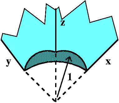
1. What does the remaining region look like? Here are several possible
pictures of the region. In this picture (sort of the corner of a
rectangular box), a spherical "bite" has been taken out of the
corner. The bite is centered at the vertex (the origin) and has radius
1. Wow!
|  |
|
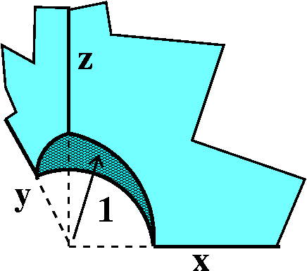
To the right is a more oblique view of the octant with the bite.
The nice thing about this region is that it can be described very briefly
in terms of spherical coordinates. Certainly, ρ will go from
1 (as close to the origin as the bite will let us get) out to ... out
to ... infinity (an improper integral!). What about θ and
φ? Here students should look closely at the definitions of θ and
φ. Each of them will go from 0 to π/2. This is best confirmed by
taking "angles" with vertex at the origin and a side along the x-
(respectively, z-axis) and then opening the second side of the angle
to an aperture of π/2 (I think "aperture" means the angle's opening).
By the way, as I remarked in class, this is actually a more realistic
example than the first integral. Things like this do occur in
electricity and magnetism. |
|
The computation
Again dm=(density)dV=[C/ρ5]dV because "density is
inversely proportional to the fifth power of the distance to the
origin." And we know the limits from the discussion above, so the
total mass is
∫φ=1φ=π/2∫θ=0θ=π/2∫ρ=1ρ=∞[C/ρ5]ρ2sin(φ)dρdθdφ.
The integrand is [C/ρ3]sin(φ) after cancelling some powers.
The inner integral
This is an improper integral, so I will be careful.
∫ρ=1ρ=BIGC/ρ3sin(φ)dρ=-C/(2ρ2)sin(φ)]ρ=1ρ=BIG=-C/(2(BIG)2)sin(φ)
+C/(2(1)2)sin(φ). As BIG→∞, the
term -C/(2(BIG)2)sin(φ)→0 so the improper
integral
∫ρ=1ρ=∞[C/ρ3]sin(φ)dρ converges and its value is
(C/2)sin(φ).
The middle integral
∫θ=0θ=π/2(C/2)sin(φ)dθ=(C/2)sin(φ)(π/2)=[(C π)/4]sin(φ).
The outer integral
∫φ=0φ=π/2[(C π)/4]sin(φ)dφ=-[(C π)/4]cos(φ)]φ=0φ=π/2=[(C π)/4]
Again, I will admit that I don't know any way to check this
answer. When such an integral comes from a real physical problem,
there is frequently some way to see if the final answer is reasonable.
Further defense of silly (the same defense)
I would only use this technique, I hope!, where both the region
and the integrand are suitable. So, although the problems may have
seemed silly, they are the sort of applications which might occur. We
will need integration in spherical coordinates a few times later in
the course.
Wednesday, October 29
A double integral
Today begins three lectures where I will attempt to describe other,
more sneaky methods to compute multiple integrals. These methods
generally are used when specific computations are given and the
regions or the integrand (the function to be integrated) share some
kinds of symmetries. All of today's examples will be relevant to
engineering education. I'll begin with the following problem. I want
to compute a double integral, something like
∫∫Rf(x,y) dA. I will describe an f and an R.
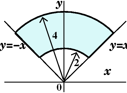 Let's let f(x,y)=x2+y2. That's certainly a
simple enough function, just a degree 2 polynomial in x and y.
Suppose R is the region in the xy-plane defined by these restrictions:
it is in the upper half plane where y>0, and it has boundary
given by y=x and y=-x (two straight lines or, actually, since they are
inside a half plane, just two rays) and the circles
x2+y2=2 and x2+y2=4. I
think, or I hope, that this region is shown in the picture to the
right.
Comments
This would be a rather unpleasant double integral to compute as an
iterated dxdy or dydx integral. I hope that you can see why. The
region R is not nicely convex in either the x or y direction, and we'd
need to break both of the iterated integrals into several pieces.
I hope that there are enough accidents (?) and coincidences (??) so
that you are a bit suspicious. Of course, this example is totally
arranged. I hope that it makes you think of polar coordinates.
 dA in polar coordinates
Here's a mostly emotional argument for how dA should be
described in polar coordinates. Later I will be able to give a more
precise derivation. Or you can look in the textbook (section 15.4) for
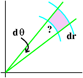
a more careful discussion.
Suppose I want to compute the area obtained by changing r to r+dr and
θ to θ+dθ. The picture displays this area, dA,
magnified a lot. As mentioned, dA is an area and has dimensions
length2. If dθ and dr are very small, the area dA is
approximately rectangular, and maybe the area is the product of the
length of its sides. Well, one side is dr but the other side is
not dθ. Angles don't have dimensions (they are ratios!)
and, anyway, if you move circles centered at the origin in and out,
you can see that the intercepted arcs change in length. These arcs are
very short close to the origin and are longer as the radius of the
circle gets bigger. In fact, the length of the intercepted arc is
directly proportional to r. This length is also directly proportional
to dθ: if the angle at the origin is doubled, the length of the
intercepted arc is also doubled. Well, "directly proportional" means
that there is some constant, uhhh ..., let's call it K, so that the
length is K r dθ. What is K? In the nicest world, K
would be 1 because then I would not have to worry about it any
more. Well, golly, that is
exactly why radian measure was invented: so this
darn constant would be 1 and
would not need attention.
Comment: so what is K and what about those words?
Why is K=1 in radians? Well, the circumference of a circle of radius r
is 2π r. Here the dθ is 2π. So apparently the K is
indeed 1. If you insisted on using degrees in all of calculus, then
the angle for a whole circle would be 360, and for
Kr dθ=K(360)r to be 2π r, you would need
K=2π/360, which is approximately the obnoxious number .01745. I
looked on the web, and the only other candidate for angle measurement
I found was the
grad, introduced in France as part of the metric system (my
calculator permits angle computations in grads). There are 400 grads
in a circle (I didn't know that) and therefore the constant K, if we
used grads in calculus, would be 2π/400 which is approximately
.01571, also obnoxious. Yes, things would be better if π were equal
to 3.
Euphemism: The expression of an unpleasant or embarrassing notion
by a more inoffensive substitute
The word "golly" is a euphemism for "God" and the word "darn" is a
euphemism for "damn".
|
 Computing the integral
Let's return to computing
∫∫Rx2+y2dA, if R is the
region shown to the right (in the upper half plane, with the curves
arcs of circles centered at the origin).
How does one recognize that the integral is "polarish"? It is a
classroom example, but the integrand has central symmetry, and so does
the region. You may be helped if you recall the conversion formulas
From r, θ to x, y      From x, y to r, θ
-------------------    -------------------
   x=r cos θ              r2=x2+y2
   y=r sin θ              tan θ=y/x
I've given the formulas the way I most often use them. In particular,
the formula for getting θ from x
and y needs to be "adjusted" (by adding π) if the point whose
coordinates are (x,y) is in the left half of the plane.
I recognize (primarily from the picture, but I can also use the
formulas) that R is described by π/4<=θ<=3π/4 and by
2<=r<=4 (Here I made a mistake in class -- the values of r go
from 2 to 4, as in the picture, not from sqrt(2) to 2! I regret the
error.) We can convert the integral into polar coordinates:
∫∫Rx2+y2dA=
∫π/43π/4∫24r2 r dr dθ=
∫π/43π/4∫24r3dr dθ=
∫π/43π/4(1/4)r4]r=2r=4dθ=(63)θ]π/43π/4=(63)3π/2.
Of course the computation is easy. It was arranged so that after
conversion to polar coordinates things would work out well. The
computation in rectangular coordinates, including finding the
boundaries of the integrals (there would have to be two of them) and
then computing the antiderivatives, would be very tedious. This is not
an entirely artificial example: it is the computation of the moment of
inertia about the origin of a thin homogeneous plate in the shape of
the region R.
The earth is flat
So here I will try to convince you by combining a valuable and
truthful computation with extremely dubious logic, that the earth is
flat. Please be reassured: the earth is probably not flat.
Newton's
Law of Universal Gravitation
Suppose I have two "point masses", m1 and m2,
which are a distance d apart. The magnitude of the force attracting
them together is directly proportional to the product of their masses
and inversely proportional to the square of the distance separating
them. The constant of proportionality is usually called G (alas, not
to recognize the lecturer!). Therefore the magnitude of the force is
G m1m2/d2.
Here's a quote from another
site:
... this constant [G] was worked out by Henry Cavendish in 1798. He
achieved this by measuring the gravitational attraction between two
1kg lead balls at a distance of 1 metre.
I would guess that you
would assume that this experiment must have found the attraction to be
very small, in fact it was so small it was a stunning achievement to
measure the tiny acceleration caused and to therefore calculate the
gravitational attractive force (using Newton's second law).
Cavendish found the force to be 6.67 x 10⁻¹¹
Nm2/kg2 (or approximately 0.0000000000667
Nm2/kg2!).
Gravity is actually much weaker than, say, magnetism. There is just a
great deal of mass around, and very few magnetic
monopoles.
|
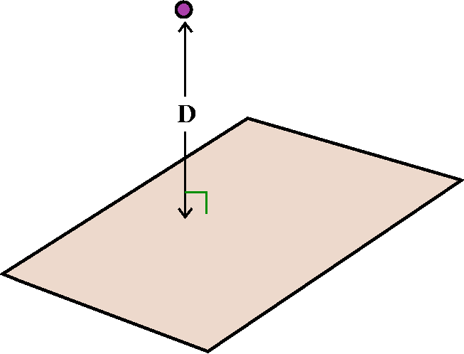 The plate: from description to integral
Let me assume that the "universe" consists of an infinite flat
homogeneous plate, and an external small object with a mass of m whose
distance to the plate is D. What is the gravitational attraction of
the object to the plate? A major part of such a problem is setting it
up. The correct location of the origin and the axes can make problems
much easier. In this case, I believe there are two reasonable
locations for the origin: the object, or the closest point on the
plane to the object. I'll use that closest point to be the origin. Of
course, the xy-plane will be the plate, and therefore the coordinates
of the object will be (0,0,D). The plate is homogeneous and thin. To
avoid having too many letters around, let me assume that the plate is
1 unit thick (otherwise I'll just have to carry around the thickness
in all of the computations, and I have a hard enough time with my own
thickness, both mental and physical). Since the plate is homogeneous
(the same at every point), it has a density, ρ. A small chunk of
the plate ("dA") located at the point (x,y) will have mass equal to
ρ dA (remember the thickness is 1, and so it is already in the
formula).
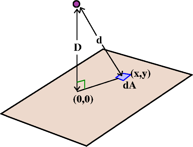
Now let us convert the ideas into more rigid "mathspeak". The
magnitude of the force from the external mass to the dA piece of the
plate is Gmρ dA/d2. The piece is located at (x,y), and
(x,y), (0,0), and the location of the external mass are at the
vertices of a right triangle. The hypoteneuse of the right triangle is
d, and the leg of the triangle from the external mass to (0,0) is
D. The distance from (0,0) to (x,y) is
sqrt(x2+y2). Therefore
d2=D2+(sqrt(x2+y2)). The square root and the square cancel. The
magnitude of the force is
Gmρ dA/(D2+x2+y2). Several
students noticed a surprising symmetry. Since we are dealing with the
whole plane, R2, the chunk of dA at (x,y) has an antipodal
chunk at (-x,-y), having the same mass and the same distance to the
external object. Therefore the "lateral" parts of the forces (parallel
to the plane) exactly cancel out. We only need to compute the vertical
component of the force.
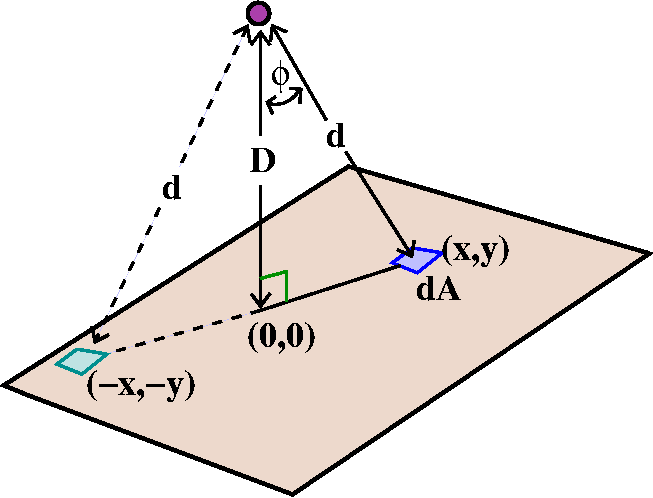 The vertical component of the force is the magnitude of the force
multiplied by the cosine of the angle, φ, between the vertical
line and the line connecting the external object to dA. But cos(φ)
is D/d, which is
D/sqrt(D2+x2+y2). The function to be
integrated is the vertical component of the gravitational attraction
between the external object and dA. This is
GmρD dA/(D2+x2+y2)3/2. Since
the plate is infinite, we want
∫∫All of R2Gmρ dA/(D2+x2+y2)3/2.
Computing the integral
Many of the letters are constants: G and m and ρ and D. We can
pull them out of the integral (but we will remember them for the final
result). We need to compute:
∫∫R2dA/(D2+x2+y2)3/2.
Since this comes immediately after a discussion of polar coordinates,
the student alert to pedagogical plans (how folks teach) will
immediately think of converting to polar coordinates. Indeed, even
those who are not so ... prescient might think: the region has
symmetry around (0,0) and the integrand has that same
x2+y2, so let's try polar coordinates!
Then dA=r dr dθ, and
r2=x2+y2, and all we need are the
limits on the integral. For the whole plane, r should go from 0 to
∞, and θ should go from 0 to 2π. The appearance of
∞ forces me to finally acknowledge that this is an improper
integral.
∫02π∫0∞r dr dθ/(D2+r2)3/2.
The inner (improper) integral
I will be careful, since I am supposed to be teaching a math course.
∫0∞r dr dθ/(D2+x2+y2)3/2=limB→∞∫0Br dr dθ/(D2+r2)3/2
The r accompanying the dr is exactly what's needed to do the
substitution u=D2+r2 with du=2r dr. We sort out the constant by guessing (maybe).
∫0Br dr dθ/(D2+r2)3/2=-1/sqrt(D2+r2)]r=0r=B=
-1/sqrt(D2+B2)-{-1/sqrt(D2+02)}
As B→∞, the term
-1/sqrt(D2+B2)→0. The other term has minus
signs which cancel, and (let's say D>0) square/sqrt which cancel,
so the limit is 1/D.
The outer integral is easy:
∫02π(1/d)dθ=(1/D)θ]θ=0&theta=2π=2π/D.
But we need to multiply by the factors we pulled out. The whole answer
is:
GmρD(2π/D)=Gmρ2π.
And, therefore ...
There is no D in the answer!. The gravitational attraction of a
flat earth is constant! Now the lecturer discussed the fact that he
weighs the same standing on the floor and standing on a
chair. Therefore ... therefore ... the earth is flat. (And even more
supporting argument: wouldn't people who wanted to lose weight climb
Mt. Everest, because they would lose weight when ...).
Discussion of the claim
Ideally, we would like more measurements rather than fewer: with
many measurements we'd have a chance of coming up with more reliable
information.
Going abstract: the "limit"
Let me look at the average a bit more. The discussion that follows seems very clever to
me.
Suppose that I assume that the number of observations is
n3 where n is a large positive integer. Then I would have
something like this:
SUM of all of the temperature measurements
------------------------------------------
                    n3
I will multiply the top and bottom of this fraction by
(b-a)(d-c)(f-e), so we would have:
SUM of all of the temperature measurements   (b-a)(d-c)(f-e)
------------------------------------------ · ---------------
                    n3                       (b-a)(d-c)(f-e)
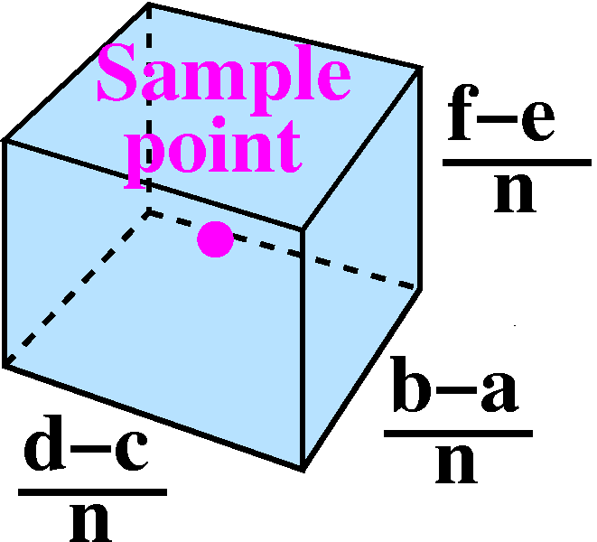 Just consider part of this, the fraction
(b-a)(d-c)(f-e)/n3. This is the same as
[(b-a)/n]·[(d-c)/n]·[(f-e)/n]. If n is large, this is
the same as splitting up each of the edges of the box into n equal
pieces, and what we have is a very small box of the ocean. Now if we
also want the points we measure to be well-distributed, then we might
expect that most of the boxes will contain exactly one sample point. We can think of
Temperature at that sample point)·[(b-a)/n]·[(d-c)/n]·[(f-e)/n]
as T(that sample point)dx dy dz or as
T(that sample point)dV where dV is this very small box
inside the huge box of ocean. When we take the SUM we actually have an approximating Riemann
sum to ∫∫∫box of oceanT(x,y,z) dV, which is a
triple integral. Whew! The limit of such approximating sums is the
triple integral, but I won't go into detail because this all parallels
a similar discussion for double integrals. I don't want to forget
anything: there is a factor of (b-a)(d-c)(f-e) remaining on the
bottom, and this is the volume of the box.
All of this is supposed to support the following definition:
The average value of the temperature in the box is
∫∫∫box of oceanT(x,y,z) dV
-------------------------
    Volume of the box
A specific example
What if our box was bounded by x=0 and x=2, y=0 and y=3, and z=0 and
z=5, and the temperature at (x,y,z) was given by the formula
T(x,y,z)=x2+7yz. Then if we wanted to compute the average
temperature we would convert a triple integral into a (triply)
iterated integral. In this case, I see no advantage in any one of the
six possible orders, so:
∫02∫05∫03
x2+7yz dy dz dx
Let's compute, from the inside out: ∫03
x2+7yz dy dz dx=yx2+(7/2)y2z]y=0y=3=3x2+(63/2)z.
∫053x2+(63/2)z dz=3x2z+(63/4)z2]z=0z=5=15x2+(63/4)(25).
∫0215x2+(63/4)(25) dx=5x3+(63/4)(25)x]x=0x=2=40+(63/2)(25).
If this were the 21st century, instead of 1872, we could type:
> int(int(int(x^2+7*y*z,y=0..3),z=0..5),x=0..2);
                                    1655/2
Incidentally, I checked and 40+(63/2)(25) is the same as (1655)/2.
This isn't the average temperature. For that we need to divide by the
volume of the box which is 2·3·5=30. The result is
(331/6).
The "moral" of this: computation of triple iterated
integrals
I don't think that there are any essential new difficulties introduced
when we move from evaluating double iterated integrals to evaluated
triple iterated integrals. Yes, there are more opportunities for error
(50% more?) but they are not new in type. So I won't devote too much
time to actual evaluation.
Describing a volume in space
Since the difficulties involved in computation of a triple iterated
integral really are just those we've seen already with double
interated integrals, I want to illustrate something that definitely
seems more complicated to me: going from a description of a region in
space over which we want to compute a definite integral to the
corresponding iterated integrals (and there are 6=3! possible ordered
for the iterated integral). Let me "integrate" (convert to iterated
integrals) the function SQUIRREL over the region in space
(R3) defined by y=0, z=3, and z=x2+y.
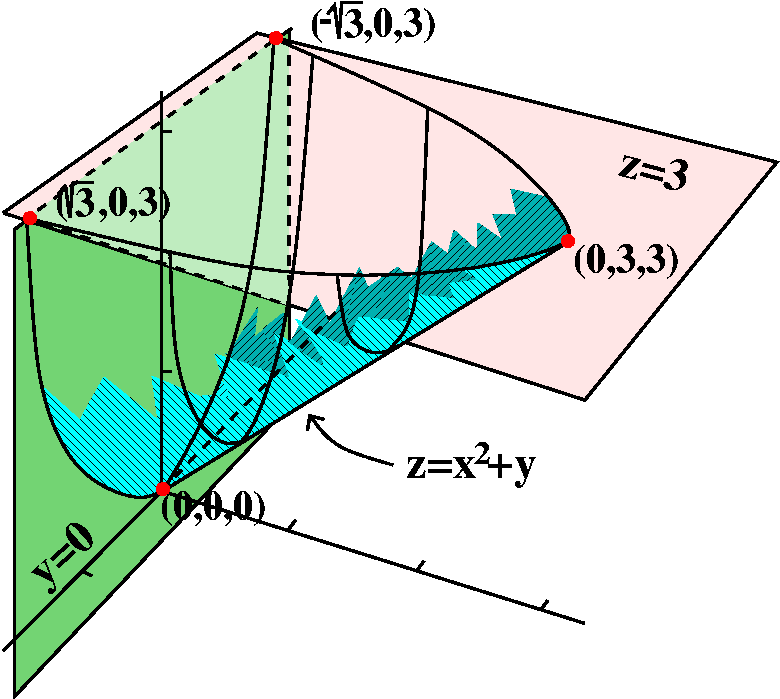 I want to
begin by sketching the region. The planes y=0 (the xz-plane) and z=3
(push the xy-pane up three units) are easy enough. The surface
z=x2+y cut by y=0 and z=3 is maybe not so obvious. When y=0
we get a parabolic arc cut off at z=3 in the xz-plane. As y increases,
the parabolic arc is translated up, but still cut off at z=3. In the
yz-plane, when x=0, the slice is a segment of the line z=y from (0,0)
(with the coordinates being y and z) to (3,3). The surface cuts the
plane z=3 with the parabola 3=x2+y or y=3-x2,
which opens "downward" (in the standard orientation of
xy-planes).
I've attempted to sketch the surface to the right of this description.
The colors are meant to show some of the curviness. There are some
extreme points which turn out to be
useful in setting up iterated integrals. Those are the points (0,0,0),
(0,3,3), (sqrt(3),0,3), and (-sqrt(3),0,3). These points are where
each of the coordinates (x and y and z) attain maximum and minimum
values on the solid region whose boundary curves were given.
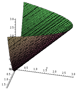 Nomenclature The surface z=x2+y is called a
tilted parabolic cylinder. It is a parabolic cylinder because
it results from a family of parallel lines in space which all meet the
parabola z=x2 in the xz-plane. It is "tilted" because these
lines are not perpendicular to the xz-plane.
Now to the right is Maple's attempt to draw the tilted
parabolic cylinder in the region of interest to us. The picture to the
right is the result of using the command:
implicitplot3d(z=x^2+y,x=-1.75..1.75,y=0..3,z=0..3,
grid=[40,40,40],axes=normal,labels=[x,y,z]);
This command did not display an immediate result on my home
computer. It requested that Maple to check a
three-dimensional grid of 403=64,000 points, and then
compute the light and the angle, etc. I rotated and chose lighting so
that I got the image displayed here. That's why "supercomputers" are
needed to draw the lighting effects for Pixar, etc.
Maple can draw ...
... some useful pictures for us when we want to look at double and
triple integrals. Last time we looked at the iterated integral
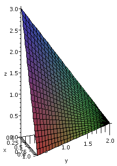
∫02∫x=0x=1-(1/2)y3-3x-(3/2)y dx dy
The command plot3d(3-3*x-(3/2)*y,x=0..1-(1/2)*y,y=0..2);
produces (after putting in the axes and making the view constrained) the graph shown to the right. I
did not know until fairly recently that Maple had the capacity to show only pictures
corresponding to double integral limits. This could be very helpful.
|
|
A region in space
Now back to the triple integral. There are six different orders that
are possible when converting a triple integral to an iterated
integral. I did three of the six orders. Let's convert
∫∫∫This regionSQUIRREL dV into various iterated
triple integrals.
dx dy dz
I'll try this order first:
∫(
∫∫
SQUIRREL dx dy)dz.
I've mentioned that my personal inclination in finding limits of
iterated integrals is working from the outside-most limit "in". There
are definitely people who are successful and do the exact opposite. I
would recommend that you find your own "natural" style and try to
follow that path. For me, I would look at the z limits first. For this
shape, I would try to find the highest and lowest z's in the spatial
region. This is not a complicated region, and we've already sketched it quite well. The highest and lowest
z's are, respectively, z=0 and z=3. So we've got ∫z=0z=3(∫∫SQUIRREL dx dy)dz.
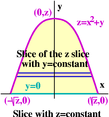 Now let's try slicing the region by z=CONSTANT, where the
CONSTANT is some unknown number between 0 and 3. This horizontal slice
of the original spatial region gets us something in the xy-plane. If
you were in class, you may recall that there was some effort involved
in sketching the slices that are shown here. But one boundary of the
sliced region is y=0, along the x-axis. The other, curved boundary, is
"inherited" from z=x2+y. Now z=CONSTANT so as a
curve in the xy-plane, if we write it in the standard
y=function of x format, we get
y=z-x2. Therefore this is a parabola (the square on x!)
opening down (the minus sign). The top of the parabola (the vertex)
occurs when x=0, and there y=z. The intersection(s) of the parabola
with the x axis occur when y=0, and there 0=z-x2, so that
x=+/-sqrt(z). The inner double integral is ∫∫
SQUIRREL dx dy. What are the bounds on the
dy integral? We must look at the slice, and see what the highest and lowest values of y are on the slice. The lowest value is 0 and highest value is z: but on the slice, z is a CONSTANT. The highest value depends on z. Now we know:
∫y=0y=z∫
SQUIRREL dx dy
Now in the region pictured, I will slice with y=CONSTANT and see how
big and how small x can be. This is a slice of a slice (maybe
[slice]2?). So the boundary is given by z=x2+y,
and with both z and y CONSTANT, I get x2=z-y, so that
x=+/-sqrt(z-y). These will be the limits on the dx integral.
So the answer is:
∫z=0z=3∫y=0y=z∫x=-sqrt(z-y)x=+sqrt(z-y)
SQUIRREL dx dy dz.
dy dz dx
Now
∫(
∫∫
SQUIRREL dy dz)dx.
Examine the original picture and the limits on the
outermost variable, x, should be revealed. The largest and smallest
x's in this region are +/-sqrt(3), and therefore we get ∫x=-sqrt(3)x=sqrt(3)(
∫∫SQUIRREL dy dz)dx. Our task is now to slice with x=CONSTANT and try
to get the other integrals' bounds.
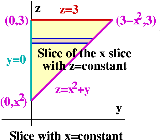
Again, once the "picture" is presented then much of the remainder of
the work is made much easier. We spent some time in class drawing this
picture. When x=CONSTANT, then certainly the slice goes through the
side (on the xz-axis) so that y=0 becomes the left boundary, if we
have z assigned to be the vertical coordinate and take y to be the
horizontal coordinate. Also the top of the region is still z=3. The
other edge is "inherited" again as the effect of the equation
z=x2+y. As I mentioned in class, it is this edge which
irritates my highly trained mathematical psychology (is there such a
thing?). Notice that x=CONSTANT, so that z=x2+y is a
straight line in the yz-plane. The slope of this line is 1. And, when
y=0, z must be x2.
The limits on the outside of the double iterated integral ∫∫SQUIRREL dy dz can now be "read off" from
the picture, since the smallest value of z is x2 and the
largest value is 3. Therefore we have the limits on the outside of the
double iterated integral: ∫z=x2z=3∫SQUIRREL dy dz. Finally, the bounds on the
dy integral are obtained by slicing the slice. So now z=CONSTANT also,
and y goes from y=0 to the right side, which is a point on the line
(it still hurts to write this when there is a square in the equation!) z=x2+y, and therefore the upper bound is y=z-x2.
So the answer is:
∫x=-sqrt(3)x=sqrt(3)∫z=x2z=3∫y=0y=z-x2
SQUIRREL dy dz dx.
dz dx dy
My last attempt:
∫(
∫∫
SQUIRREL dz dx)dy.
Again, the picture shows that y in the solid region
varies from 0 to 3, and we've got 2 of the 6 limits (o.k., the easiest
of them): ∫y=0y=3(
∫∫
SQUIRREL dz dx)dy. The y=CONSTANT slice should give the other information.
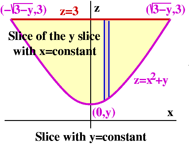
Again, the picture gives much of the information we need. Drawing the
picture was some work. Here with y=CONSTANT, the top of the slice is
caused by the plane z=3. The bottom of the slice is
z=x2+y. Now since x is a variable, this is indeed a
parabola. The parabola opens up (positive coefficient on the square
term) and has vertex (0,y): the first coordinate is x and the second
coordinate in this slice is z. The parabola intersects the line z=3
when 3=x2+y. Since y=CONSTANT, this occurs when
x=+/-sqrt(3-y). The outer, x-limits, on the double integral will be
x=-sqrt(3-y) and x=+sqrt(3-y). Now slice the slice, for make
x=CONSTANT also. z will vary. The highest value of z will be 3 on the
[slice]2. The lowest value of z is given by
z=x2+y.
The final way the poor SQUIRREL is chopped up and then
summed is
∫y=0y=3∫x=-sqrt(3-y)x=+sqrt(3-y)∫z=x2+yz=3SQUIRREL dz dx dy.
Comments
First, this is a classroom example. The solid region is actually not
very complicated. It is a convex region with boundaries given
by low-degree polynomials. The word convex means that line
segments whose ends are in the region always have the whole line
segment in the region. The problem would be much more complicated
if the functions defining the boundary weren't so simple, or if some
of the slices weren't convex (then we'd need to split up the
integrals, etc.). I remarked in class and I'll repeat here that the
process of finding these limits seems to be difficult, and hard to
describe -- I don't know yet of a computer program which can do it
reliably.
Here are the "answers" again:
∫z=0z=3∫y=0y=z∫x=-sqrt(z-y)x=+sqrt(z-y)
SQUIRREL dx dy dz
∫x=-sqrt(3)x=sqrt(3)∫z=x2z=3∫y=0y=z-x2
SQUIRREL dy dz dx.
∫y=0y=3∫x=-sqrt(3-y)x=+sqrt(3-y)∫z=x2+yz=3SQUIRREL dz dx dy.
I can't immediately see that the darn limits describe the same volume
in R3. Maybe you can. But you should see, just looking at
the patterns of the answers, what sorts of limits are "legal" and what
are not. You can only have variables in the limits if they haven't
been integrated yet. For example, in the last answer, the lower limit
of the innermost integral is z=x2+y, and the outside two
integrals are dx and dy. I could not have a limit in, say, the middle
integral of the form z=x2+y because there would be only one
variable left to be integrated, and there isn't any way to "kill" both
x and y. So there is a rough guide to the grammar (?) of the bounds on
iterated integrals.
How can you check this kind of "computation"?
Generally checking these things can be difficult and tedious. Luckily,
we are in the 21st century and I have powerful
friends. Well, I guess I can ask some electrons to run around. Look at
the following:
> W:=x^6*y^8*z^2;
                                      6  8  2
                                W := x  y  z

> int(int(int(W,x=-sqrt(z-y)..sqrt(z-y)),y=0..z),z=0..3);
                                            1/2
                              417942208512 3
                              -----------------
                                 5763232475

> int(int(int(W,y=0..z-x^2),z=x^2..3),x=-sqrt(3)..sqrt(3));
                                            1/2
                              417942208512 3
                              -----------------
                                 5763232475

> int(int(int(W,z=x^2+y..3),x=-sqrt(3-y)..sqrt(3-y)),y=0..3);
                                            1/2
                              417942208512 3
                              -----------------
                                 5763232475
I specified a "random" function, W, to replace
SQUIRREL. I wanted the antiderivatives not to be a
problem, so I just specified some powers of x and y and z. I asked
Maple to compute the triple iterated integrals in all three
ways we found. The answers are shown. They are such large and silly
numbers, and they all agree exactly. I am fairly confident the bounds on
the iterated integrals are correct.
How clever? Not very clever ...
I could have specified W=0, and then I bet the computation would have
returned 0 for all of the setups, and this answer would not be very
helpful. I could have specified W=1 and would have gotten
(24/5)sqrt(3), the volume, for all of the setups. That would be
fine. In fact, I confess that the first W that I tried was actually
x3y7z2. Why wasn't this a very clever
choice, and what was the answer I got? Hint: 3 is odd and this
region in space is ...
|
Something for you to do ...
Choose one of the other three orders and write the triple iterated
integral for that order. You can't integrate SQUIRREL without more specificity, so
all you can do, and what I would like, is to write the precise
bounds. Here are what I think are the answers:
∫z=0z=3∫x=-sqrt(z)x=sqrt(z)∫y=0y=z-x2
SQUIRREL dy dx dz
∫x=-sqrt(3)x=sqrt(3)∫y=0y=3-x2∫z=x2+yz=3SQUIRREL dz dy dx
∫y=0y=3∫z=yz=3∫x=-sqrt(z-y)x=sqrt(z-y)SQUIRREL dx dz dy
Wednesday, October 22
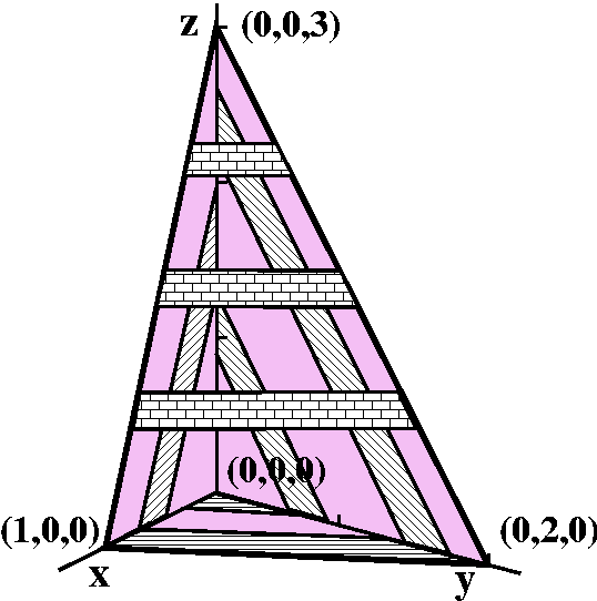 Volume of a tetrahedron
A tetrahedron is a flat-sided object with four corners. I would
like to compute the volume of a tetrahedron whose corners are at
(0,0,0), (1,0,0), (0,2,0), and (0,0,3). There are several ways to
compute this volume, including some which need no "calculus", just
vector manipulation (using the triple product formula, for
example). To the right is an attempt at a picture. It shows the
corners (the four vertices) and the faces, and I've made some attempt
to show the four sides with differently decorated "stripes" on
each. There are four flat sides. There's one on each coordinate plane
(xy-, yz-, xz-) and there is a tilted face. The equation of the tilted
face (the points (1,0,0) and (0,2,0) and (0,0,3) are on the tilted
face) is x+(y/2)+(z/3)=1. And I got this equation totally by guessing.
Here we'll use a double integral to find the volume of the
tetrahedron here. I think of this solid as lying over a triangle in
the xy-plane. The triangle is determined by (0,0), (1,0), and
(0,2).The height of the solid over this triangle is z=3-3x-(3/2)y,
which I got from the equation for the tilted face, just by solving it
for z.
As a double integral
So the volume is ∫∫BaseHeight dA, and
this is ∫∫The triangle3-3x-(3/2)y dA. I'll convert
this to an iterated integral to compute it.
47 second break for theory
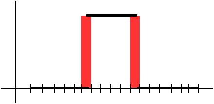 In one variable calculus, as I explained last time, the initial
glimpse at the theory in back of the definite integral assumes that
the function doesn't have any jumps. But real functions can
jump! The functions which are met in mechanical engineering (just hit
something!) can certainly look like what's shown to the right. And
similarly, functions met in digital signal processing really can look
like that also. They certainly can be integrated. The secret is that
the jumps really don't matter very much. They can be put inside little
boxes where the variation doesn't matter very much (the red boxes in the picture). So the sums defining the
definite integral still approach a limit, the "correct" limit.
Here I am apparently not even worrying about the domain. Well, this is
what we could do if we had another 30 minutes to fritter away on
details. I could define a function piecewise in this way:
F(x,y)=3-3x-(3/2)y if (x,y) is in the triangle, and F(x,y)=0 if (x,y)
is not in the triangle. Suppose R is any rectangle in the xy-plane
which contains the triangle. The the volume of the tetrahedron would
be ∫∫RF(x,y) dA. I hope that you will see this
double integral is the same as the double integral over the triangle
that I'll compute by looking at iterated integrals. The
discontinuities of the piecewise-defined function turn out to give a
perturbation of the Riemann sums which →0 as the size of the pieces
→0.
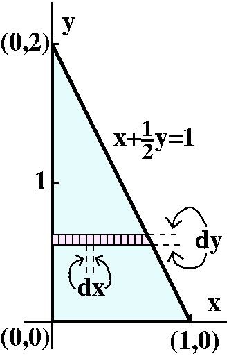 Converting to iterated integrals
Let's write ∫∫The triangle3-3x-(3/2)y dA as a
dx dy iterated integral. That means figuring out the bounds on
the integrals.
I will work from the outside in. So first I need to get the lowest and
highest values of y in the triangular base:
∫Lowest yHighest y∫???3-3x-(3/2)y dx dy
There's a sketch of the base to the right, and the sketch declares
that the Lowest y is 0 and the Highest y is 2. Now I
imagine (and frequently draw, as shown on the sketch!) a very thin
collection of dx by dy rectangles being added up in a row across the
region. It is so thin that y is almost constant and the x's range from
the leftmost edge to the rightmost edge. The left edge is certainly 0
always. But the right edge depends on y. When y is very near the
bottom (y=0), the right edge is very near 1. When y is near the top
(y=1), the right edge is near 0. What is the relationship between x
and y on this edge? Of course the edge reflects the tilted face of
the tetrahedron, which has the equation x+(y/2)+(z/3)=1. On the base,
z=0, so the equation giving the tilted side of the triangular base
must be x+(y/2)=1. Therefore x on the rightmost edge is given by
x=1-(1/2)y. Here is the resulting iterated integral:
∫02∫x=0x=1-(1/2)y3-3x-(3/2)y dx dy
Even thought it is not logically necessary (because the dx dy
notation does determine what variable is integrated first), I do tend
to write "x=" on the limits of the inner integrals. This may save me
from confusion and error as I compute.
Computing the iterated integral
I'll first compute the inner integral:
∫x=0x=1-(1/2)y3-3x-(3/2)y dx=
(antidifferentiate with respect to x, so y is a constant here!)
3x-(3/2)x2-(3/2)yx]x=0x=1-(1/2)y=
3{1-(1/2)y}-(3/2){1-(1/2)y}2-(3/2)y(1-(1/2)y)-0. The -0 comes from the lower limit, x=0. I tend to expand and "simplify" here. So we get:
3-(3/2)y-(3/2){1-(1/2)y}2-(3/2)y(1-(1/2)y)=3-(3/2)y-(3/2){1-y+(1/4)y2}-(3/2)y+(3/4)y2=
(3/2)-(3/2)y+(3/8)y2
Now the outer integral:
∫02(3/2)-(3/2)y+(3/8)y2dy=(3/2)y-(3/4)y2+(1/8)y3]02=(3/2)(2)-(3/4)(4)+(1/8)(8)=1.
I remarked in class that, maybe it should be "clear" to me that the
volume is 1, but it isn't.
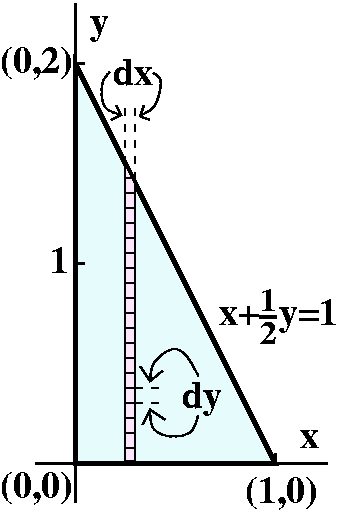 The other iterated integral
Now, just to practice, we'll write ∫∫The triangle3-3x-(3/2)y dA as a
dy dx iterated integral.
Again, I will work from the outside in. So first I need to get the
leftest (leftmost) and rightest (rightmost) values of x in the
triangular base:
∫Leftmost xRightmost x∫???3-3x-(3/2)y dy dx
Now the base triangle is again shown to the left, but with the kind of
"doodles" that I would make suitable to finding the limits of a
dy dx iterated integral. The leftmost value of x is 0 and the
rightmost value of x is 1. Now my dx by dy triangles form a vertical
strip where x is just about constant. For the inner limits on y I need
to know that the strip goes from the bottom, where y=0, to the
top. The top will vary, depending on x. The equation of the boundary
line for the top is the same: x+(y/2)=1. Now we need to know y as a
function of x. So solve for y and get y=2-2x. That's the upper limit
on the dx integral. Here is the resulting iterated integral:
∫01∫y=0y=2-2x3-3x-(3/2)y dy dx.
Computing the iterated integral
I'll first compute the inner integral:
∫y=0y=2-2x3-3x-(3/2)y dy=
(antidifferentiate with respect to y, so x is a constant here!)
3y-3xy-(3/4)y2]y=0y=2-2x=
3(2-2x)-3x(2-2x)-(3/4)(2-2x)2-0. Again, the -0 comes from the lower limit, y=0. Now expand and simplify:
6-6x-6x+6x2-(3/4){4-8x+4x2}=3-6x+3x2
The outer integral:
∫013-6x+3x2dx=3x-3x2+x3]01=3-3+1=1.
Thank goodness, we got 1 again.
Possible sources of error in these computations
I'm looking ahead a little bit here. We will discuss triple integrals
next time, and these are also usually computed by a transition to
triple iterated integrals. There are six possible orders for iterated
triple integrals. I make errors frequently. The prominent sources of
error include: antidifferentiating with respect to the wrong variable,
substituting for the wrong variable, and, well, general
confusion. Please try to guard against these. You may make these
errors, and just do the computation again, and try to keep your
composure intact ("Keep cool, y'know!").
By the way, although I wanted our first example to be as easy as
possible, when I was typing up the diary notes above, I ... made
several errors and had to go back and redo things. Oh well.
Another one
The base of a solid is the region in the first quadrant of the
xy-plane bounded by the curve y=x2 and the line y=3x. The
height over the xy-plane is given by
z=x6y7. Find the volume of this solid.
The double integral is ∫∫BaseHeight dA, and
this is ∫∫The shapex6y7 dA.
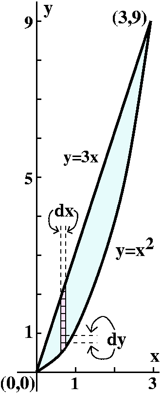
One iterated integral, with its computation
We will convert this first to a dy dx integral. The outside
limits come first. The most left x gets on the base is x=0. The most
right x gets is x=3. We know this because we graphed the base, and
found the intersection points of y=x2 and y=3x by solving
3x=x2, which has roots at x=0 and x=3. Therefore the
iterated integral looks like:
∫03∫???x6y7dy dx
What about the limits on y? Here the sketch of the base, together with
my doodles, may be useful. The vertical strip of boxes tells me that I
should add up things from y=x2, the lower bound, to y=3x,
the upper bound. Therefore this iterated integral is:
∫03∫y=x2y=3xx6y7dy dx
Now to compute the integral. The inner integral:
∫y=x2y=3xx6y7dy=(1/8)x6y8]y=x2y=3x=(1/8)x6(3x)8-(1/8)x6(x2)8.
This "simplifies" to
(1/8)38x14-(1/8)x22. (I am using the
powerful rules of exponential manipulation here!) And now the outer
integral:
∫03
(1/8)38x14-(1/8)x22dx=
(1/8)38(1/15)x15-(1/8)(1/23)x23]03=
(1/8)38(1/15)315-(1/8)(1/23)323=(1/8)323([1/15]-[1/23]). Wow!
The other iterated integral, with its computation
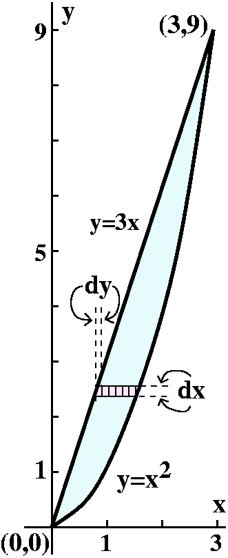 Now for the dx dy integral. The highest and lowest values for y
are 0 and 9. Therefore the integral must be:
∫09∫???x6y7dx dy
Now we need to consider a (fixed) y slice through the base. The
left-hand side of that fixed y slice is determined by y=3x and the
right-hand side of the slice is determined by y=x2. We need
to know the limits on x in terms of y. So we need to know
x=Left(y) and x=Right(y). That means "solving for x" in the boundary
equations. This (here, in this classroom example!) is not too
hard. y=3x becomes x=(1/3)y on the left, and y=x2 becomes
x=sqrt(y) on the right. The positive square root gets used here
because (picture!) we're in the first quadrant. The iterated integral
is:
∫09∫x=(1/3)yx=sqrt(y)x6y7dx dy
The computation begins with the inner integral.
∫x=(1/3)yx=sqrt(y)x6y7dx=(1/7)x7y8]x=(1/3)yx=sqrt(y)=
(1/7){sqrt(y)}7y7-(1/7){(1/3)y}7y7=(1/7)y7/2y7-(1/7)(1/3)7y7y7
This now "simplifies" (what a silly word!) to
(1/7)y(21)/2-(1/7)(1/3)7y14. Now the
outside:
∫09(1/7)y(21)/2-(1/7)(1/3)7y14dy=
(1/7)(2/(23))y(23)/2-(1/7)(1/3)7(1/15)y15]09=
(1/7)(2/(23))9(23)/2-(1/7)(1/3)7(1/15)915=
(1/7)(2/(23))323-(1/7)(1/3)7(1/15)330=
(1/7)(2/(23))323-(1/7)(1/15)323=(1/7)323([2/(23)]-[1/15])
(1/7)(1/16)325-(1/7)(2/(23))323=
(1/7)323{(1/16)-2/(23))
Theorem
 1     / 1      1  \     1    / 1      2  \
--- · | ---- - ---- | = --- ·| ---- - ---- |
 8     \ 15     23 /     7    \ 15     23 /
The proof consists of observing that the dx dy and
dy dx values of the double integral must be equal by the Fubini
result, and then dividing both values by 323. (The student
may, of course, verify this statement using the tools of third grade
arithmetic, but the prestige of double integrals is ... [priceless?].)
This "theorem" may be the silliest statement of the course.
Pi? The Bible??
Some students objected when I tried to write Pi instead of 3 as I was
assembling information for the computation above. I cited the Bible as
a reference. Here
is information about the "history of Pi" including specific biblical
citations. Since we are at a secular university, I give this not for
its religious value, but for ... uhhhh ... historical context. Also,
maybe ... uhhhh ... maybe the value of Pi has changed with time. Uhhhh
... also everyone should know a few digits of Pi. This
reference discusses how the computation of the first
trillion or so decimal digits was done. You can search the
first four billion bits (binary digits) of Pi for patterns here.
More on difficulties and on the psychology of the individual
Please don't panic. If you want to compute a double integral, you
don't need to do both iterated integrals -- just one of them. I
chose to do both to show you how (I hope!).
Notice that we needed to go from one description of the boundary
curves: {y=3x, y=x2}, to another: {x=(1/3)y,x=sqrt(y)},
when we did dx dy after dy dx. "Solving" (finding a
convenient form for inverse functions) may be difficult (or even
impossible in terms of familiar functions).
One last remark: I almost always try to find the bounds on iterated
integrals going from the outside-most integral to the inside-most
integral. Some people may find the transition from inside to outside
more easy (this difference in approach will be more emphatic when we
do triple integrals). You should try a series of examples and settle
upon what you find most comfortable. And remember that you can always
"change" to the other way.
By the way ...> int(int(x^6*y^7,x=(1/3)*y..sqrt(y)),y=0..9);
31381059609
-----------
115
> int(int(x^6*y^7,y=x^2..3*x),x=0..3);
31381059609
-----------
115
So Maple gets the same answer both ways, also.
 Integrating Frog over a region
If the integrand (the function to be integrated) is not too weird,
then I hope you should be convinced that the actual
antidifferentiations probably aren't the essential difficulty. The
difficulty is more in setting up the iterated integrals:
finding the bounds. Here is a more complicated example.
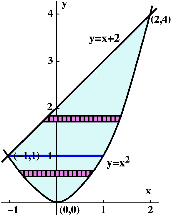
The region R is bounded by y=x+2 and y=x2. What does this
region look like? Well, this is a problem in a calculus course, so
solving x2=x+2 shouldn't be impossible. In fact, this leads
to x2-x-2=0 which is (x-2)(x+1)=0 so intersections occur
when x=-1 (so y=(-1)2=1) and when x=2 (so
y=22=4). I would like to integrate Frog over the region R:
∫∫RFrog dA. More precisely,
I'd just like to set up the bounds of the iterated integrals which are
equal to this double integral.
Totally randomly, dx dy first
This wasn't a random choice. The dx dy order introduces an
additional kind of complexity. Consider these limits:
∫Bottom of yTop of
y∫x=Left(y)x=Right(y)Frog dx dy.
The Top of y and Bottom of y are easy enough. In the region R, the
smallest y value is 0 and the largest y value is 4. Now think about
x=Left(y) and x=Right(y). The thick horizontal
blue line in the sketch separates different formulas for
the Left limit of x as a function of y. Below it, the Left limit is
determined by the left-hand side of the parabola. Above it, the Left
limit is determined by the straight line. Theoretically this does not
cause any problems. But when you're actually trying to compute
everything, what people usually do is separate the pieces:
∫01∫x=Left(y)x=Right(y)Frog dx dy +∫14∫x=Left(y)x=Right(y)Frog dx dy.
In the first iterated integral, as y goes from 0 to 1, the left and
right boundaries are both given by formulas related to
y=x2. Here x=+/-sqrt(y), so Left(y)=-sqrt(x) and
Right(y)=+sqrt(x). In the second iterated integral, y goes from 1 to
4. Here also Right(y)=+sqrt(x), but Left(y) comes from y=x+2, so
Left(y)=y-2. So the dx dy iterated integrals which are
equal to the double integral are:
∫01∫x=-sqrt(y)x=sqrt(y)Frog dx dy +∫14∫x=y-2x=sqrt(y)Frog dx dy.
Now dy dx
This one is much easier. I can read off the left and right extreme
values of x, and then the y boundary values are given by the equations
which already "present" the region R. I don't need to split up
things. Here it is:
∫-12∫y=x2y=x+2Frog dy dx.
Almost surely, unless circumstances were very strange, I would set up
the iterated integral this way and not in the dx dy way.
The New
Jersey Chorus Frog, Pseudacris feriarum kalmi, is an
endangered species in some of its
range.
In my office ...
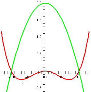
A student visited me and we did some more Frog-like problems (one with Toad and one with Lizard. Let me show you the Lizard problem. The region we looked at was
bounded by y=2-2x2 and y=x4-x2. A
Maple graph with these two functions is shown to the right.
Just as in the previous (Frog)
example, writing the dy dx integral is quite direct. My student
visitor and I wrote iterated integrals for the other
order: dx dy. You can try this problem. First, though, think a bit
and see how many iterated integrals will be necessary.
Hint
I think three pieces are needed. Notice that
y=x4-x2 is the same as
x4-x2-y=0 and this is
(x2)2-x2-y=0, a quadratic in
x2. So you can "solve" for x2 using the
quadratic formula, and then take square roots of the resulting answers
to get 4 possible values of x for each value of y. Certainly this is a
mess, but this is possible to do without extravagantly advanced
methods.
|
A problem from a calculus textbook
This problem shows one further "wrinkle" that can occur with double or
triple or any kind of "multiple" integral. Here's the statement:
Evaluate the double integral ∫∫Dex/ydA, where D={(x,y)|1<=y<-2,
y<x<=y3}.
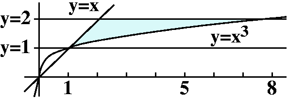 As to why this problem introduces a new kind of complexity, I invite
you to ask Maple to integrate ex/y both dx and dy.
That is, what are the respective antiderivatives? The x antiderivative
is yex/y but ... there is no y antiderivative in terms
of familiar functions. So if we want to get an answer to the
textbook's problem, we'd better first do dx and then leave dy until
later. The dx dy double integral is easy enough to write, because the region D is described suitably:
∫12∫x=yx=y3ex/ydx dy
The inner antidifferentiation gives
∫x=yx=y3ex/ydx=yex/y]x=yx=y3=yey3/y-ye1=yey2-ey
and then ∫12yey2-ey dy is just
(1/2)ey2-(e/2)y2]12=(1/2)e4-2e.
Comment I do know some examples, in "real" applications, not
textbooks, where looking at the order of the iterated integrals
changes something really nasty into a function which can be handled
routinely. So, although this is a textbook/class example, it does show
an idea which may be useful.
Monday, October 20
Quick review of the definite integral in calc 1
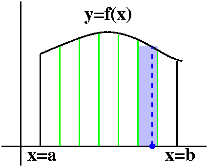 Suppose we have a nice function f(x) of one variable defined on and
interval, [a,b]. We might want to find the area under y=f(x) on that
interval, althogh that is more of an excuse to define the definite
integral than a real ambition. Here is one approach to the
definition. Take a large positive integer n and divide [a,b] into n
equal parts each of width
 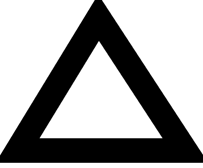 x=(b-a)/n. In each subinterval choose a sample point, say
qj in the jth subinterval. Compute the sum
∑j=1nf(qj)
 x. This is a Riemann
sum approximating the definite integral. As n-->infinity, any
sequence of sums is supposed to approach a unique limit, and that
limit is the definite integral. But there are many choices of sample
points, and maybe it isn't clear that the choices don't influence the
limit. So what if we take another point pj in the
jth subinterval as a sample point? Then since the width is
Δx, certainly |qj-pj|≤
 x. The Mean Value Theorem (let me
assume that f is differentiable) then says there's some constant, C,
so that |f(qj)-f(pj)|≤C
 x. (I'm not too
interested in the details here -- we're only skimming!) But we can
estimate the difference when different choices of sample points are
made:
|∑j=1nf(qj) x - ∑j=1nf(pj)
 x|≤nC
x|≤nC x
x x.
x.
The "n" comes because
there are n pieces in the sum. One of the  x's occurs because
that's a common factor in both sums. The other comes from the MVT
estimate we just stated. But now, since
  x=(b-a)/n, we see that
the estimate of the difference is C(b-a)2/n. Two of the n's
cancel. We are left with an n on the bottom, and this means that the
Riemann sums do get closer as n→∞, no matter what choice of
sample point is made.
Theorem For any choices of sample points, as n→∞, the
Riemann sums→a unique limit, the definite integral of f from a to b,
and written ∫abf(x) dx.
Of course the integral sign and the dx's are notation to remind people
of the approximating sums. We could approximate the definite integral
with Riemann sums, and of course there are many other numerical
approximation schemes. But the champion method is:
FTC If F´=f, then ∫abf(x) dx=F(b)-F(a).
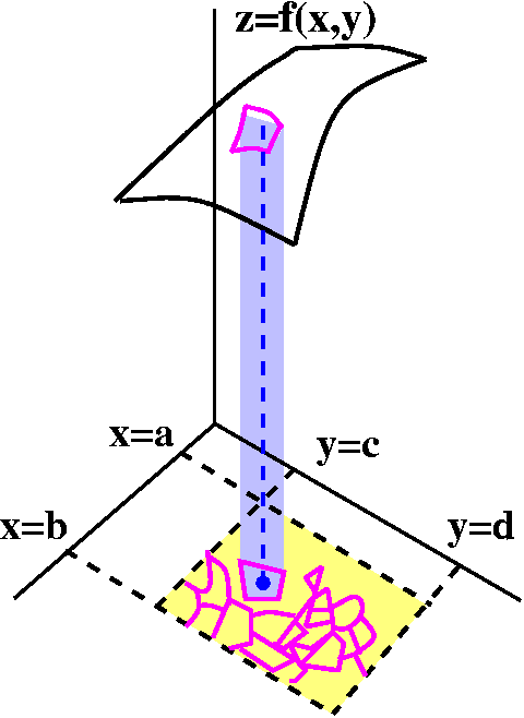
Defining the double integral
In fact the definition more or less parallels the single integral
definition. I'll follow the text closely here. We begin with a nice
function (say, continuous) defined on a rectangle R in R2
with bouindaries x=a, x=b, y=c, and y=d. Chop up the area of the
rectangle into a bunch of chunks. In each chunk, choose a sample
point. Compute the corresponding Riemann sum, the sum over all the
chunks of f's value at the sample point multiplied by the area of the
chunk. If f(x,y)>0 on R, then this Riemann sum approximates the
volume under z=f(x,y) and over R. Then it's true that as the maximum
size of the chunks→0, the Riemann sums→a unique limit. This
limit is the double integral over R of f(x,y): ∫∫Rf(x,y)dA. This
is a mathematical abstraction of the volume. The volumes computed as a
result of formulas in earlier calculus (solids of revolution, solids
with simple cross-sections, etc.) take advantage of symmetry. The
theoretical tool defined here allows us to compute volumes without any
simple kinds of symmetry. As I mentioned in class, numerical
computations of double integrals (and other higher-dimensional
creatures) are sometimes necessary, but the computations get much more
intricate than the simple ideas shown in calc 2.
Almost all the computations of volumes that I've made in my life have
occurred as a result of teaching third semester calculus. Maybe the
following is a bit more interesting.
Mass of a plate
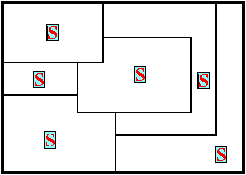 Maybe this is a more realistic "scenario". Suppose you are given a
thin rectangular metal plate with an unknown density
distribution. Therefore this is not necessarily a homogeneous
thin plate. The plate is too heavy or too unwieldy to weigh directly,
and you need to estimate the total mass. Also the mass distribution --
the density -- is not necessarily given by a simple formula. What
maybe could be done is tiny Samples taken at various parts of the
plate, according to some method (maybe depending on accessibility or
expense or ... anything). Then these samples could have their density
measured, and maybe then, after dividing the plate (thoughtwise!) into
pieces, the sample densities could be multiplied by the areas of the
pieces. The sum of these products would then be an estimate for the
mass in the plate. (It is a Riemann sum.) If a better (more accurate?)
estimate was wanted, maybe then use more sample points, smaller areas,
etc. The process is exactly the same mathematics as the definition of
the double integral.
Reality?
Well, you might work for Schlumberger and your sample points
might cost three to five million dollars each as you try to
investigate the oil or gas quantities of some region. You'd then
really think a bit about the whole process. And that's what they do.
|
Some very simple examples of double integrals
Example A The rectangle R is defined by x=3 and x=7 and y=5 and
y=8. The function is f(x,y)=700. Then ∫∫Rf(x,y)dA is 700(7-3)(8-5). Of course, I am using the
fact that the volume described by the double integral is the volume of
a rectangular solid with edge dimensions 700 and 7-3 and 8-5.
Example B Here I took f(x,y) to be
5-x2+y2, definitely a more complicated function
than the previous example's. The rectangle I took was defined by x=-3,
x=3, y=-3, and y=3. Let's temporarily discard the 5 and concentrate on
-x2+y2. If I interchange x and y the sign of the
function's value changes. But the rectangular domain is symmetric
about (0,0), so the net value (+'s and -'s cancelling!) of the double
integral of -x2+y2 over the rectangle is 0
(!). Now I "integrate" the 5, and the result is 5(3-(-3))(3-(-3)). So
we did have a more complicated function but the choice of domain made
the hard part of the function drop out.
Basic properties
The basic properties of the double integral are exactly like those of
the 1-dimensional version.
- Linearity If f and g are both nice functions defined on the rectangle R,
then ∫∫Rf(x,y)+g(x,y)DA=∫∫Rf(x,y)dA+∫∫Rg(x,y)dA; if k is a constant, then ∫∫Rkf(x,y)dA=k∫∫Rf(x,y)dA.
- Order If f(x,y)≤g(x,y) for all points (x,y) in the
rectangle, then ∫∫Rf(x,y)dA≤∫∫Rg(x,y)dA.
|
How to compute?
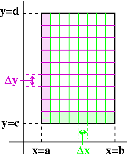 Maybe all this theory is very nice, but let me show you the way most
double integrals are computed. One method of chopping up a rectangle
is to use vertical and horizontal lines, parallel to the sides. So we
get a grid of subrectangles, each
  x by
x by  y, with both
 's very small. In addition to
choosing this special chopping strategy we could also decide to add up
the contributions (the f(sample point)
 x
x y) in an orderly manner. So, for example, we could add up the
contributions from the lowest "row" first. In that row, since
  y is small, y hardly varies at
all. The sum of a row sure looks like the definite integral with
respect to x only for "that" value of y. The same can be done for each
row. When the row sums are done, we now have the y's to worry
about. But this is a y integral. Of course, a completely symmetric
procedure can be used in the other order: first dy, with x held
constant, and then dx. Again what's here is not a "proof" but I hope
the discussion supports the following result.
Fubini's Theorem
Suppose f(x,y) is a continuous function in a rectangle R defined by
x=a, x=b, y=c, and y=d. Then
∫∫Rf(x,y)dA=∫cd∫abf(x,y)dx dy=∫ab∫cdf(x,y)dy dx.
Comments The first "creature" in the equation above is called a
double integral. The two others are officially called
iterated integrals: iterated means "repeated". Technically and
precisely these integrals are different creatures. Also please note
that the outside integration limits go with the outside d-variable --
sometimes this can be confusing. When it is, I write things like "x=a"
instead of just "a" so I don't confuse myself.
Example 1
Let me try to compute
∫∫R x3y7dA where R is the
rectangle defined by x=1, x=4, y=2 and y=5. The Fubini Theorem allows
me to "trade in" the double integral for an iterated integral, either
dx dy or dy dx. There are some occasions where one order or
the other might be preferable (we'll see this later) but here I don't
think that happens. So:
∫∫Rx3y7dA=∫25∫14x3y7dx dy.
I'll begin by computing the inner integral:
∫14x3y7dx=(1/4)x4y7]14.
In this antidifferentiation, the y7 is a constant (this is,
not surprizingly, exactly the inverse of partial
differentiation). Then we evaluate and get
(1/4)44y7-(1/4)14y7=(255/4)y7.
I remarked in class that I sometimes lose my way in these
computations, and need to write
(1/4)x4y7]x=1x=4
to insure that I remember to substitute for the correct variable.
Now ∫25(255/4)y7dy=(255/4)(1/8)y8]25=(255/4)(1/8)58-(255/4)(1/8)28.
My silicon buddy ...
A report from Maple:
> int(int(x^3*y^7,x=1..4),y=2..5);
                                   99544095
                                   --------
                                      32
Example 2
Let's try a random function: f(x,y)=sqrt(3x+8y). Well, this isn't so
random (as you'll see!). I just wish I had thought of it in class. The
rectangle I have in mind has these boundary lines: x=0 and x=3 and y=0
and y=2. In the previous example we converted the double integral into
a dx dy iterated integral. Let me try a dy dx order here. I
think that either order, again, is about the same amount of work.
So let's try:
∫∫Rsqrt(3x+8y)dA=∫03∫02sqrt(3x+8y) dy dx.
The inner integral is ∫02x3sqrt(3x+8y) dy. We
need a "dy" antiderivative of sqrt(3x+8y). Here we can really
get confused! To me writing the function as (3x+8y)1/2
makes the problem easier. I guess that the antiderivative will
be something close to (3x+8y)3/2. Well, but I need to
multiply by stuff to get rid of the various constants. For example, I
need to multiply by (2/3) because of the power. And I need to multiply
by (1/8) because of the coefficient of y that the chain rule will push
out. So the answer is (2/3)(1/8)(3x+8y)3/2, and we must
substitute:
(2/3)(1/8)(3x+8y)3/2]y=0y=2=
(2/3)(1/8)(3x+16)3/2-(2/3)(1/8)(3x+0)3/2, and
this is (1/12)(3x+16)3/2-(1/12)(3x)3/2.
And now the outer integral:
∫03(1/12)(3x+16)3/2-(1/12)(3x)3/2dx=(1/12)(1/3)(2/5)(3x+16)5/2-(1/12)(1/3)(2/5)(3x)5/2]03=
{(1/90)(3·3+16)5/2-(1/90)(3·3)5/2}
-{(1/90)(3·0+16)5/2-(1/90)(3·0)5/2}=
(1/90)(255/2-95/2-165/2+0)=
(1/90)(55-35-45)=
(1/90)(3125-243-1024)=(1858/90)=(929/45).
Well, y'see, everything was chosen so
that the final answer would have no square roots. Isn't that
wonderful!
Or, in the 21st century ...
> int(int(sqrt(3*x+8*y),x=0..3),y=0..2);
                                      929
                                      ---
                                      45
Exams returned
The exams were returned. Grading information is available, a version of the exam can be
inspected, as well as some answers to tha version.
Wednesday, October 13
We studied the following problem from 1 variable calculus:
Consider the ellipse x2+5y2=1. Find the
rectangle of largest area inscribed in this ellipse with sides
parallel to the coordinate axes. Of course this turns into: maximize
4xy (the objective function) subject to
x2+5y2=1 (the constraint). Consideration
of the geometry (varying rectangles) suggests that there is indeed a
"biggest" rectangle, somewhere.
How the "heck" does a calc 1 student solve this problem since the
function to be maximized, 4xy, has two variables.
I suggested the following methods of solution:
- Reduction of dimension, simple version
Since
x2+5y2=1, we know that
y=sqrt((1-x2)/5). Then the area is
F(x)=4x·sqrt((1-x2)/5). The domain for this function is
0=<x=<1. General theory from one variable calculus states that
max/min are obtained at end points or critical points. But
F(0)=F(1)=1. So the max is gotten where F'(x)=0. We computed this.
Of course, in a random situation, it may be very difficult to
solve (effectively!) for one of the variables in terms of the other.
- Reduction of dimension by parameterization
We could make an
inspired "guess": try x=cos(theta) and y=sin(theta)/sqrt(5). Then the
pair (x,y) is on the ellipse, and since the max is obtained somewhere
in the first quadrant, we are left with maximizing
4xy=(4/sqrt(5))cos(theta)sin(theta)=(2/sqrt(5))sin(2theta) for theta
between 0 and Pi/2. This can be solved almost "by inspection": just
take theta to be Pi/4. The max value is then 4/sqrt(5). Of course, in
a "random" situation it may be very difficult to get nice
parameterizations.
- A weird way to do the problem
I had Maple sketch some level curves of 4xy, the
objective function, and compare them with the constraint curve
x2+5y2=1. Here is the result of these
Maple commands.
A:=contourplot(x*y,x=-1.1..1.1,y=-1.1..1.1,color=red,
thickness=2,scaling=constrained,grid=[50,50],
contours=[.02,.05,.08,.2,.3,.5,-.02,-.05,-.08,-.2,-.3,-.5]):
B:=implicitplot(x^2+5*y^2=1, x=-4..4,y=-4..4,color=blue,
thickness=2, scaling=constrained, grid=[80,80]):
display({A,B});
The picture is shown to the right. |
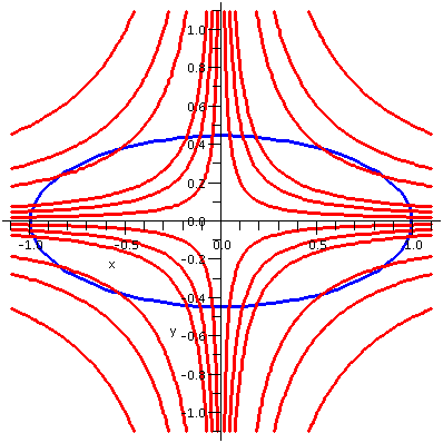 |
A close-up view
Suppose you consider a level curve of the objective function that
crosses the constraint curve, as shown. One math word which
applies to this situation is that the two curves are
transversal. So we have 4xy=C crossing
x2+5y2=1. What happens if we "wiggle" C a
little bit, so we consider 4xy=C+epsilon and 4xy=C-epsilon. Now it
seems reasonable (4xy is certainly continuous, so its values don't hop
around or break or anything) that these level curves are close to
4xy=C. These level curves must also cross the constraint
curve. That means the function 4xy has values C+epsilon and C-epsilon
on the constraint curve. (The level curves are exactly where that
function takes on its values!) Since there are both larger and smaller
values of 4xy on the constraint curve, C can't be an extreme value
(either max or min) for 4xy on x2+5y2=1.
|
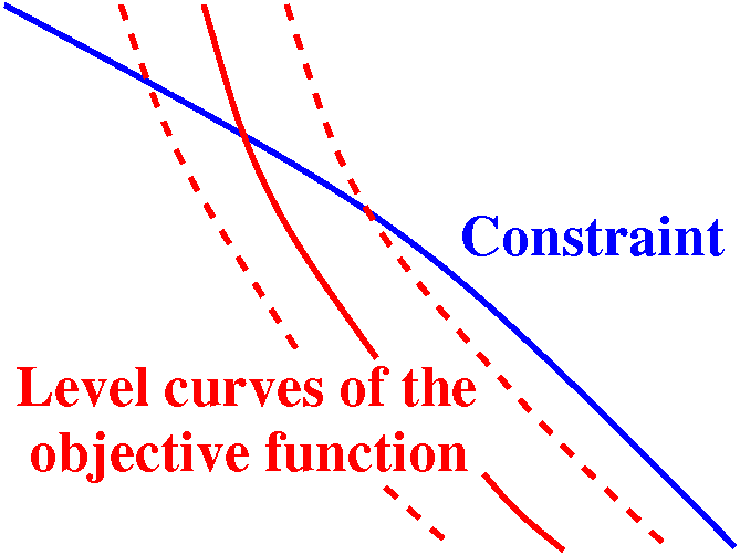
Local picture near a level curve
corresponding to a non-extreme value |
Another close-up view
This seems to imply, if you examine the picture closely, that the
largest (and the smallest) values of 4xy will be at points on the
ellipse where the ellipse will be tangent to level curves of the
constraint, x2+5y2=1. If the level curves of the
objective function are not tangent, then we will be able to vary the
values of the constant generating that contour and get bigger and
smaller values of the objective function on the constraint curve.
If the level curves are tangent then the normal vectors of the
constraint curve (∇f at that point) and the objective function
(∇g) at that point will both be perpendicular to the same line (in
three dimensions it would be a tangent plane). These gradient
vectors may not be exactly the same vector, but one of them must be a
scalar multiple of the other.
|
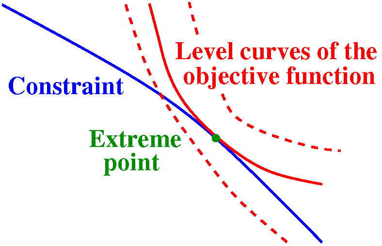
Local picture near a level curve
corresponding to an extreme value |
Now the algebraic side
If f(x,y)=4xy and g(x,y)=x2+5y2=1, then at such
points (extreme values of the objective function on the constraint
curve), there is some real number
λ so that ∇g=λ
∇f (everyone uses this Greek letter) because the tangent
lines are the same, and therefore the normal vectors must be parallel:
one must be a scalar multiple of the other. This one vector equation
in R2 gives two scalar equations, one for each component of
the vectors: 2x=(λ)4y
10y=(λ)4x
This, together
with the constraint equation g(x,y)=x2+5y2=1
gives a system of 3 equations in 3 unknowns. We can solve this by, for
example, solving for λ in each
of the first two equations and setting them equal. We need to watch
out for spurious solutions or evasions of solutions. These may occur
when we divide by certain variables. This gave us another way to solve
the maximization problem, a method which is more in the spirit of
several variable calculus. It turns out that this strange idea is
actually quite useful in "real world" problems. The method is called
Lagrange multipliers
and is discussed in section 14.8 of the text. The
method is used extensively in economics and in many areas of
engineering.
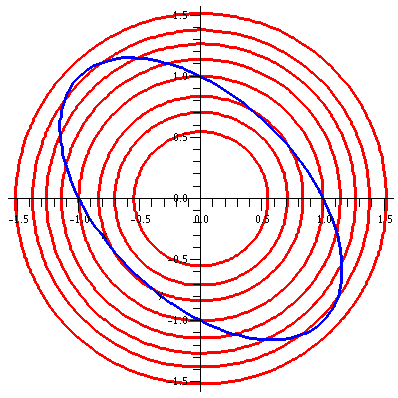 Example #1
Here the constraint is x2+xy+y2=1, and the
function to be maximized, the objective function, is
x2+y2. The picture corresponding to this
situation is shown to the right.
The bigger circles correspond to larger values of the objective
function.
Suppose that T(x,y)=x2+y2 were the temperature
in a thin metal plate with shape the interior of
x2+xy+y2=1, where will the plate be hottest or
coldest? I remind you that in this "heat" language the level curves or
contour lines are called isothermals.
Well, local extrema only occur at critical points, and
only (0,0) is a c.p. That, easily, is the coldest point in the
plate. But where is the hottest point? It must be on the edge, and it
will NOT be a local extremum, but only an extremum for a
constrained maximization. We seek therefore the extrema on the boundary
using Lagrange multipliers.
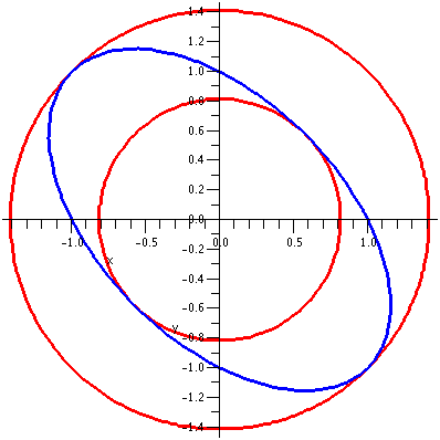 Compute the gradients, etc.
Then the multiplier equations and the constraint equation
are:
2x+y=(λ)(2x)
2y+x=(λ)(2y)
x2+xy+y2=1
Again we can solve with (2x+y)/(2x)=(2y+x)/(2y) so x=+/-y (and
possible special cases of x or y being 0). And so the temperature is
going to be T(x,y)=2 or 2/3 since
x2+xy+y2=1 gives x2=1 or
x2=1/3. There are no solutions with x or y equal 0, because
if one of them is 0 then the other is also 0 (using the two multiplier
equations) and the point (0,0) does not satisfy the third equation.
Here is a picture of these special isothermals T(x,y)=2 and
T(x,y)=2/3, and the constraint.
Fan mail for the Lagrange multiplier method
I think it is wonderful that a relatively small amount of
algebraic effort can produce such a lovely geometric result (the
specific circles centered at (0,0) which are also tangent to the
ellipse). This reassures me that things algebraic and geometric both
reflect the same reality.
Example #2
Find the maximum and minimum values of 3x-4y+5z on the unit sphere
x2+y2+z2=1. Here is perhaps a more
complicated picture, with the constraint (the unit sphere) and five
planes representing where f(x,y,z)=3x-4y+5z=-8 and -3 and 1 and 5 and
9. The picture is supposed to help you understand that max/min occur
where the planes will be tangent to the sphere.
The system of Lagrange multiplier equations (three of them here, since
we are in R3) together with the constraint follows.
2x=3(λ)
2y=-4(λ)
2z=5(λ)
x2+y2+z2=1
The left-hand sides are the components of ∇(x2+y2+z2)
and the right-hand sides are λ multiplying the components of
∇(3x-4y+5z).
You can solve for x and y and z in terms of λ, and
substitute these values in the constraint equation, getting
λ=+/-(2/sqrt(50)). Then 3x-4y+5z turns out to be (for the two
choices of λ, generating two candidates for where extreme values
take place) sqrt(50) and -sqrt(50). Here a final picture of the
constraint and the two planes given by 3x-4y+5z=+/-sqrt(50).
|
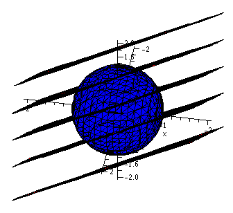
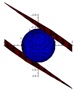
|
Proofs, etc.: the dual (?) nature of math
I learned and "liked" Lagrange multipliers in a several variable
calculus course, just as I hope you are. The justification for the
method was more or less what I have shown you. So I knew it was
"true". But I never saw a "proof" of the Lagrange multiplier method
until my second year of grad school. Sigh. It really isn't that
difficult to prove. Maybe I didn't (even as an apprentice professional
mathematician!) feel the need to prove such a lovely idea.
More examples
I discussed in detail some more complicated examples when I taught an
honors version of this course. Here
is a link to an algebraic analysis of the examples. The examples
are complicated, and some
complicated pictures of them can be viewed here.
|
Wednesday, October 8
Review of 1 variable
I try not to work hard, so I thought maybe a quick review of extreme
value material from 1 variable calculus would be useful. The names of
ideas to recall include these:
maximum, minimum, absolute maximum, absolute minimum, local maximum,
local minimum.
Fermat's fact
What I called "Fermat's fact" was the following wonderful observation
in one-variable calculus:
If f is differentiable at x0
and if f´(x0) is not 0, then f does not have an
extreme value at x0.
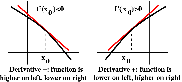
The picture shows a "proof" (well, I hope fairly convincing to a
picture person). If there is a tilt in the tangent line, then there
are both higher and lower values near x0. If x0
is either kind of extreme value (max/min), then we see that
f´(x0) cannot be 0.
Critical number
Therefore the following definition is written.
x0 is a critical number of the function f
if either f is not differentiable at x0 or
f´(x0)=0.
For simplicity in this discussion I'll assume that f is defined in some
interval that has x0 inside it (in the interior).
Identifying ("classifying") the type of critical point
Last time we saw the 68th derivative test. The idea was to
use Taylor's Theorem and then use the (crazy) hypotheses to make a big
chunk of the Taylor polynomial vanish. The function then qualitatively
resembled the next term of the Taylor series.
And now let's look at more than 1 dimension: maximum, minimum,
absolute maximum, absolute minimum, local maximum, local
minimum. These words and phrases mean more of less then same, but the
max/min situation in more than one variable is much more
complicated. Some examples will be useful.
The simple pictures with simple formulas
Here are some pictures and some formulas.
| Discussion and formulas | The pictures |
|---|
Min
A function defined on all of R2 with a local (and absolute)
minimum is f(x,y)=x2+y2. The graph of this
function is a surface called a paraboloid. It is a nice, smooth
"cup" opening up. Vertical slices through (0,0) are all parabolas
opening up and the contour lines are circles.
The red dot is the critical point and
the brown plane is the tangent plane
at that point (the xy-plane).
|
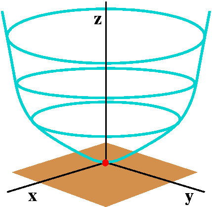
|
Min
The simplest local and absolute strict maximum is, of course, just the
reflection of the previous example, done with minus signs
algebraically. So here f(x,y)=-x2-y2, and (0,0)
provides a strict maximum. The graph is a paraboloid whose axis of
symmetry is again the z-axis. This graph opens "down".
|
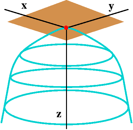
|
A saddle
The function f(x,y)=-x2+y2 gives a nice example
of a saddle point. The xz-slice (where y=0) shows the curve
z=-x2 and the yz-slice (where x=0) shows
z=y2. Each has a (strict) extreme point at 0. One is a max
and one is a min. Such behavior is called a saddle
point. Perhaps the behavior most similar in one variable calculus
would be that of the function x3 (an inflection point). But
in 2 and more variables the local situation can be much more
complicated.
Here the surface is more complicated, and my picture is certainly not
so good. But the tangent plane and critical point are the same. The
tangent plane cuts through the surface (similar to the way a tangent
line at an inflection point in 1 variable calculus cuts through the
graph of a curve).
|
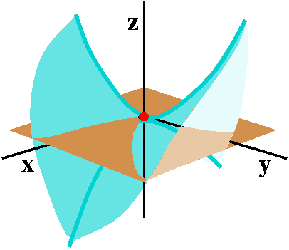
|
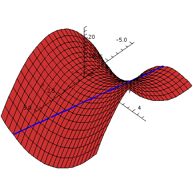 Ridiculous interesting (?) fact
The surface z=-x2+y2 is what's called a ruled
surface. The word "rule" comes from an older version of English, and
here means "straight line".
Every point on the surface is on a straight line which sits entirely
in the surface. I didn't believe this when I was told it for the first
time, and maybe you don't either. For example, the point (1,2,3) is on
this surface (since 3=-12+22) and the line whose
parametric equation is x=1+t, y=2-t, and z=3-6t goes through that
point and sits entirely on the surface. Such surfaces have
applications in computer graphics.
You can verify algebraically that the line whose parametric equations
are given above is on the surface, or you can look at the picture to
the right, which shows the saddle together with the line: nearly
silly.
|
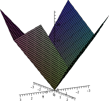 A surface with corners?
I wanted to give an example of a function which might make you think a
bit. Consider f(x,y)=|x+3y|+|5x-y|. This is a strange function, but it
is easily computed. For example,
f(4,-2)=|4+3(-2)|+|5(4)-(-2)|=10+22=32. So computationally, this is an
easy function. To the right is the result of this Maple command:
plot3d(|x+3*y|+|5*x-y|,x=-3..3,y=-3..3, axes=normal,grid=[75,75])
The grid option makes the program sample
at 75·75 points in a rectangular arrangement. This is much more
than the default value, and will usually make the sketch of the
surface more accurate. It can take much more computing time and
storage, however.
I claim that this function has an absolute minimum at (0,0). Why?
Certainly f(0,0)=0. And if the value of f equals 0, then (since
absolute values are always non-negative) both x+3y and 5x-y must be
0. The only solution of the system of equations x+3y=0 and 5x-y=0 is
(0,0) (this is either "high school math" or sophisticated linear
algebra) so f(x,y)>0 for all (x,y) which are not (0,0).
Using Fermat's fact here
If a point is a local extreme point of some function f in several
variables, and if that function is differentiable at that
point, then all of the first partial derivatives of the function must
be 0 at that point. If that's not true, just "slice" the function at
that point in the direction of the derivative which is not 0. The one
variable Fermat fact implies that the function does not have an
extreme value (max or min) at the point in one variable, and therefore
the function in several variables has both higher and lower values
near the point. Therefore (whew!):
An extreme point must be a critical point.
Our functions will almost always be differentiable (not like the graph
with corners above), so our functions will have their extreme values
where ∇f=0.
Definition of critical point
Suppose f is a function of n variables. Then f has a critical
point at p in Rn if either ∇f doesn't exist at p (so
at least one of the first partial derivatives fails to exist) or
∇f(p)=0 (the zero vector, remember!).
In this course, almost all the functions we'll consider will be
differentiable. This doesn't mean that non-differentiable functions
(functions with jumps or corners) are not important or interesting in
mathematics and its applications (again: linear optimization, shock
waves in physical phenomena). Just learning to use the tools for higher
dimensional analysis of differentiable functions is a big enough
task.
Another instructor's final exam question
Suppose
f(x,y,z,w)=3x6+8y12+55z8+9w64.
What are the critical points of f and what type (max, min, saddle) are
they?
As I remarked, this problem seems a bit forbidding. Bug
fx3·6x5. The only way this is 0 is for x
to be 0. Similar remarks for fy, fz, and
fw imply that the only critical point for this function is
(0,0,0,0).
What type of critical point is (0,0,0,0)? Well, f(0,0,0,0)=0. And if
any of the coordinates in (x,y,z,w) is not 0, then (since we have only
even powers!) f(x,y,z,w)>0. Therefore this critical point is an
absolute minimum.
Suppose z=f(x,y), and f is differentiable. What is the geometric
meaning of "(x0,y0) is a critical point of f"?
Since ∇f(x0,y0)=0, both of the first partial
derivatives are 0. Therefore z=f(x0,y0) (that
is, z=a constant) is the tangent plane to z=f(x,y) at the point
(x0,y0,f(x0,y0)). The
"flat" plane through the point, parallel to the xy-coordinate plane,
is tangent to the surface. This can be difficult to "see" in a graph,
though.
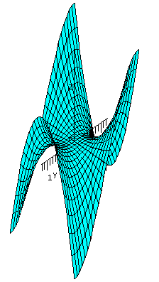 Monkey saddle
The examples already shown are the standard critical points for
functions of two variables. But there are many, many other kinds of
critical points. The graph z=x3-3xy2 shows one
of them. Again the origin, (0,0), is the only critical point. This is
because zx=3x2-3y2 and
zy=-6xy. For zy to be equal to 0, either x or y
must be 0. But then use zx=0 to conclude that the other
variable must be 0 also. For this function, the xy-plane is the
tangent plane at the origin because (0,0,0) is on the graph. This
critical point's local behavior is up/down repeated three times (at
equally spaced 120o angular intervals) if you walk around
the surface in a small circle centered at the origin. The critical
point is called a monkey saddle because, presumably, a monkey
could sit on it with spaces for two legs and a tail to hang
down.
Critical points of more than one variable can have many, many
different local pictures, and there has been a great deal of effort
expended trying to understand them.
|
Taylor's Theorem in two variables
Here is a result:
f(x,y)=f(x0,y0)+
fx(x0,y0)(x-x0)+fy(x0,y0)(y-y0) +
[1/2!](fxx(x0,y0)(x-x0)2+fyx(x0,y0)(y-y0)(x-x0)+fxy(x0,y0)(x-x0)(y-y0)+fyy(x0,y0)(y-y0)2) +
ETC.
Here the first line is the constant term, the second line has the
first-order (degree 1) terms, and the third line consists of the
second-order (degree 2) terms. Of course, the third line (because
mixed partials are equal) is actually only
fxx(x0,y0)(x-x0)2+2fxy(x0,y0)(x-x0)(y-y0)+fyy(x0,y0)(y-y0)2).
If (x0,y0) is a critical point, then the linear
(first order, degree 1) terms are 0. We can expect and hope that the
shape of the degree 2 terms maybe looks like f near
(x0,y0). The problem is that these degree 2
terms can themselves be a bit hard to understand. Here are pictures
of three polynomials of degree 2 in x and y.
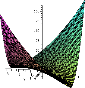 |
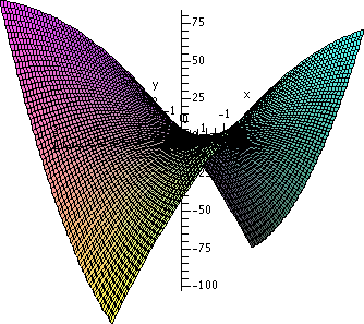 |
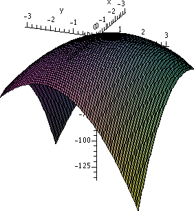 |
| 5x2-10xy+3y2
I think this one is a saddle.
| -4x2-10xy+3y2
Another saddle (there are lots of saddles in this business!).
|
-4x2-5xy-6y2And this seems to be a maximum. |
Now a second derivative test in two variables
There's one second derivative test which is usually "given" to
students in a third semester calculus course. It is a bit
complicated. The test essentially results from computing the second
directional derivative at the critical point and seeing how to ensure
that this result is always positive (or always negative or ...). That
together with results from one variable calculus (on concavity) will
insure some kinds of local behavior near the critical point. There is
a description in the book, but I want to concentrate on stating the
result and then giving some examples. That is enough of a task!
Second derivative test for two variables
Suppose f(x,y) is a differentiable function, and
(x0,y0) is a critical point. That is,
fx(x0,y0)=0 and
fy(x0,y0)=0. Then compute
D=fxx(x0,y0)fyy(x0,y0)
-(fxy(x0,y0))2. Here we go:
| If D>0 |
and if
fxx(x0,y0)>0 then f has a local minimum at
(x0,y0). |
and if
fxx(x0,y0)<0 then f has a local maximum at
(x0,y0). |
| If D<0 then
f has a saddle point at
(x0,y0). |
| If D=0 then
this second derivative test supplies no information.
|
Please note that when D>0, the signs of fxx and
fyy must agree (as I said in class, this is not
obvious!) so that you can check either of these numbers. The textbook
calls D the discriminant. It is also called the Hessian
in some places. Also I mentioned that I think of D as the determinant
of this:( fxx fxy )
( fyx fyy )
Looking at D this way turns out to lead to second derivative tests
in more than 2 variables.
Problem 19 of section 14.7
We are asked to "find the critical points of the function. Then use
the Second Derivative Test ..." and the function in problem 19 is
f(x,y)=x-y2-ln(x+y).
Let's find the c.p.'s. Since fx=1-(1/[x+y]) and
fy=-2y-(1/[x+y]) we knw that 1-(1/[x+y])=0 and therefore
x+y-1=0. In fact, x=1-y. Use this in the second equation,
-2y-(1/[x+y])=0 by substituting for x. The result is -2y-(1/[1-y+y])=0
so that -2y-1=0 and y must be -1/2. Since x=1-y, x=1-(-1/2)=3/2. The
only critical point for this f is (3/2,-1/2).
Important note Solving non-linear equations can really be quite
difficult, and each collection of such equations can present different
"challenges". Any method that gets a solution is a good method, and
there's likely to be more than one good method!
Now let's use the Second Derivative Test. We know fx and
fy. So we can compute fxx=1/(x+y)2,
fxy=1/(x+y)2,
fyx=1/(x+y)2, and
fyy=-2+1/(x+y)2.
A silly note about a habit of mine Since I sometimes make
mistakes computing derivatives, I usually compute both
fxy and fyx and quickly see that they're
equal. This provides a small check in this computation.
At the critical point, (3/2,-1/2),
D=fxxfyy-[fxy]2=1·(-1)-12=-2,
so this critical point is a saddle point. Luckily this is an
odd-numbered problem in the textbook, and I can quickly check (as I
just did) that this answer is correct!
Euler's example
Leonhard Euler (1707–1783) was a great and very prolific
mathematician. He published Institutiones Calculi
Differentialis (In English, Methods of the Differential
Calculus) in 1755. It was an influential text, and was the first
source of criteria for discovering local extrema of functions of
several variables. In it Euler investigated the following specific
example: V=x3+y2-3xy +(3/2)x. He asserted that V
has a minimum at both (1,3/2) and (1/2,3/4). Was Euler correct? (My
source for this information is A History of Mathematics by
Victor J. Katz, Harper Collins, 1993, p.517.)
Let's compute. Vx=3x2-3y+{3/2} and
Vy=2y-3x. Critical points occur where both Vx
and Vy are 0. There 2y=3x or y= {3/2}x, so the
Vx condition becomes: 3x2-{9/2}x+{3/2}=0 or
6x2-9x+3=0 which factors (even then textbook problems were
predictable!) into (2x-1)(3x-3)=0. The critical points are as Euler
asserted: (1,{3/2}) and ({1/2},{3/4}). Logically just checking that
Euler's points are critical points is not enough -- we should
check that he found all critical points, which we did.
Now to test the type of the critical points: Vxx=6x,
Vxy=-3, Vyx=-3, and Vyy=2. So the
discriminant is the determinant of
(6x   -3)
(-3    2)
which is 12x-9. At (1,{3/2})
this is 12-9>0, and Vxx=6>0, so this
critical point is a local minimum. At ({1/2},{3/4}), the discriminant
becomes is 12·{1/2}-9=-3<0, which
makes this critical point a saddle point. Euler was wrong!
Testing the monkey saddle
This shows another weakness of
the Second Derivative Test. If z=x3-3xy2, then
we saw that the only c.p. was (0,0). Here
zx=3x2-3y2 and zy=-6xy, so
that zxx=6x, zxy=-6y, zyx=-6y, and
zyy=-6x. When x=0 and y=0, all of the second partial
derivatives are 0, so that D=0. The Second Derivative Test returns
no information. This test says "saddle" only when the
function has a second-order saddle point -- any other type of
saddle behavior forces D=0. A second-order saddle goes up/down/up/down
as you walk around the critical point, and the second-order saddle has
D<0. So in a number of ways, the Second Derivative Test has
problems. It can also be difficult to compute by hand, for example, as
some examples below indicate.
|
Two more functions
There are two amazing and disconcerting examples. At least, to me
these problems are both amazing ("surprise greatly; overwhelm with
wonder" -- well, at least the first) and disconcerting ("disturb the
composure of; agitate; fluster" -- certainly they show me I don't
understand too well what can happen in "space"). The results show some
huge differences between 1 and 2 dimensions.
One strange example
The function
f(x,y)=-(x2-1)2-(x2y-x-1)2
is given. This is not the world's most horrible function. It is "only"
a polynomial of degree 6. Let me find the critical points.
Well,
fx=-2(x2-1)2x-2(x2y-x-1)(2xy-1) and
fy=-3(x2y-x-1)x2.
Consider the equation fy=0 first. Well, maybe x=0. Then
fy=0 and fx=0-2(-1)(-1) is not 0. So this
doesn't get me any critical points.
Now to get fy=0 we can ask that x2y-x-1=0. Then
fx=0 becomes (x2-1)2x=0 since the other piece
becomes 0. Then either x=0 or x=1 or x=-1. Whew! If x=0,
x2y-x-1=0 becomes -1=0: false. If x=1, x2y-x-1=0
becomes y-2=0 so y=2. Therefore (1,2) is a critical point. If x=-1,
x2y-x-1=0 becomes y=0, and (-1,0) is a critical point.
If you don't like this logical torture, try the following:
> f:=-(x^2-1)^2-(x^2*y-x-1)^2;
                               2     2     2           2
                       f := -(x  - 1)  - (x  y - x - 1)
> solve({diff(f,x),diff(f,y)});
                        {x = 1, y = 2}, {x = -1, y = 0}
Yup, two critical points. Below are two very local pictures of
the graphs near the critical points.
 The pictures certainly shouldn't be convincing evidence, but they do
seem to support the assertion that the function has local minimums
at both critical points! (We can verify this assertion with the second
derivative test but this is too much work for me right now.)
Why do I find this disconcerting? Well,
imagine we walk from one peak to another (shown to the right, the
blue "trail"). Shouldn't we somehow pass through a saddle? Well, in
fact, no, we don't need to: maybe the lowest point on the blue trail
is not a critical point -- the tangent plane to the surface at that
point may be tilted. In this example, the tangent plane is
always tilted at every point except the two peaks.
Shouldn't we somehow pass through a saddle?
|
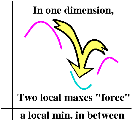
The situation in 1 variable calculus is considerably different.
If I
have two local maxes (and, yeah, if the function is continuous,
differentiable, etc.: nice) then there must be a local min between
them.
|
Another strange example
Here f(x,y)=3xey-x3-e3y. Then we
compute fx=3ey-3x2 and
fy=3xey-3e3y. If fy=0,
then ey3(x-e2y)=0 so x=e2y (the other
factor, ey, is a value of the exponential function and is
never 0). Then fx=3ey-3x2=0 leads to
3ey-3(e2y)2=0 or
ey-e4y=0 or
ey(1-e3y)=0. Since exp is never 0, we need
1=e3y and this occurs only when y=0. Therefore this
function has only one critical point, at (1,0).
My friend does this, by the way:> f:=3*x*exp(y)-x^3-exp(3*y);
3
f := 3 x exp(y) - x - exp(3 y)
> solve({diff(f,x),diff(f,y)});
2 2
{x = 1, y = 0}, {x = RootOf(_Z + _Z + 1), y = ln(-1 - RootOf(_Z + _Z + 1))}Since I know that z2+z+1 has no real roots (the
discriminant is 12-4·1·1=-3<0) this
function has exactly one critical point. And the formula for
the function isn't really that horrible, either.
The left graph below is a local picture of the critical point. This
seems to convincingly support the assertion that (1,0) is a
local strict maximum of the function. (We can verify this assertion
with the second derivative test but I am too lazy.) In the graph on
the right, x goes from -5 to 5 and y varies just between -.05 and .05:
therefore y is just about 0, and
3xey-x3-e3y is just about
3x-x3-1. Certainly this shows that the function has no
absolute max or min.
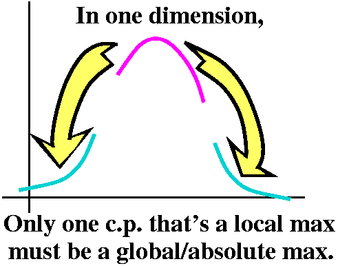 The situation in 1 variable calculus is considerably different.
Suppose we have a function defined on all of the real numbers (o.k., a
differentiable function) which has exactly one critical point
and that critical point is a local maximum. Then that local
maximum is a global, absolute maximum for the function. What the
heck is happening in several variables? I just don't
understand, that is, really understand beyond superficially. |
|
Monday, October 6
The handout
I tried to give each student a copy of this handout. I sincerely thank the
gentleman (name?) seated towards the back who gave some late entering
students copies.
Do we understand the handout?
I remarked that I used unusual variable names and some new
notation. The new (?) variable names and notation represent my effort
to get you to think about the logic behind all the notation. As we
will see later, sometimes the notation in this subject seems almost
intentionally designed to obstruct understanding!
The first table on the handout had the information below. f
and g are declared to be differentiable functions of two variables.
  M     N  f(M,N) D1f(M,N) D2f(M,N)  g(M,N) D1g(M,N) D2g(M,N)
 -1    -2     6      4        0         3      8       1
 -1     2     2     -2        1        -5      7       6
  1    -1    -2     -5        4        -2      9       4
  1     2     5     -7        6        -1     -2       7
  2     1     0     -1       -2        -3      7       4
So M and N specify inputs to the functions f and g. Therefore f's
value when, say, M=1 and N=2, is 5: f(1,2)=5. What are the
D1 and D2 columns? This is another notation for
partial derivatives, notation which some people prefer when there
might be confusion about how the variables are named. D1
would refer to the partial derivative with respect to the first
variable (frequently we have called this x) and D2 is the
second variable (usually called y). Therefore in more traditional
notation, ∂f/∂x(1,2)=-7 and ∂g/∂y(-1,2)=6.
The second table on the handout referred to values to two
differentiable functions of one variable.
  v  h(V)  h´(v)  k(v)  k´(v)
 -2   5     2      3     5
  0   0     2     -2     7
  1   1     3      2    -1
  2  -1     4      4    -2
Maybe this table (in spite of the choice of variable name: v!) is a
bit easier to understand. The value of the function k at input 1 is 2,
and k's derivative at 1 has value -1. Also, h(0)=2 and h´(0)=3.
Doing the problems
A sequence of four problems were given. Let's try them.
Club suit: ♣
If S(t)=h(k(t)), compute S(1) and S´(1).
This is one variable calculus. But let me try to think about it a bit
first:
Thinking about it
I can think about the function S as a sort of box, which takes inputs
and processes them in some fashion, and produces outputs. The S box
also has some internal structure. The input first is sent to box
representing the k function, and then the output from that (sub?)box
is sent to the h function. If we follow through (using values from the
second table) we can see that 1 "changes" to 2 and then to -1.
What about the derivative? The derivative is a multiplier of a
tiny change in the input. It signals the first order change in the
output compared to the input. In the case of S, if we "kick" the input
by c (think of c as a small number) then 1+c is fed into the k
box. The output will be approximately (neglecting H.O.T., higher order
terms) 2 (the old output) +k´(1)c, which is 2+(-1)c. Now feed in
2+(-1)c. If c is small, (-1)c will be small. The output from the h box
will be -1 (the old output, what h "does" to 2) plus a change. The
first order part of the change will be a proportionality constant,
h´(2), multiplying the kick that is passed to the h box. The kick
passed to the h box is (-1)c, so the compounded effect is that h's new
output (approximately, first order) is -1 (the old value of h's
output) plus h´(2)(-1)c=4(-1)c.
Now go "up" a logical level. The input, 1, to S was kicked to 1+c. The
S output, to first order, is -1 (the old output) plus
4(-1)c. Therefore the derivative of the S box at 1 is 4(-1), since the
derivative is the multiplier of the kick.
The diagram below is supposed to be visual "support" of the
preceding discussion.
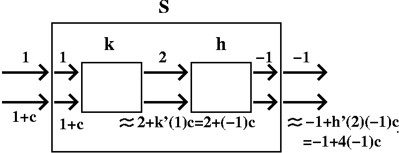
A formula
If S(t)=h(k(t)), the one variable chain rule states that
S´(t)=h´(k(t))k´(t), so S´(1)=h´(k(1))k´(1)=4(-1).
Formulas are good!
Diamond suit: ♦
If W(t)=f(h(t),k(t)), compute W(1) and W´(1).
Thinking about it
Now the W box has a different structure. The input is split
(bifurcated -- what's the point of being in an academic environment if
a silly, uncommon word isn't used in place of one that would be
understood!) into two, and each is fed separately into h and k
boxes. The outputs, now in order, are carefully put into f. The output
from the f box is then pushed outside as the value of W.
To compute W(1), we find h(1)=1 and k(1)=2, and then compute
f(1,2)=5. Easy (?)..
What about the derivative? Suppose we kick 1 to 1+c. The response of
the one variable boxes, h and k, should not be difficult to
understand: the outputs, linearized, are 2+k´(1)c=2+(-1)c and
1+h´(1)c=-1+3c, respectively. It is important to remember which
output is which! Now feed this into f. The multiplier for
perturbations in the first variable is D1f(2,1), so the
effect of the change in the first variable adds on
D1f(2,1)(-1)c to the output. The second variable
contributes in proportion to its perturbation, with the constant of
proportionality being D2f(1,2), so D2f(1,2)(3)c
gets added on. If we look up the numbers and do arithmetic, we can see
that the total (linearized) effect (neglecting higher order errors!)
is 5 (the old output) plus 25c. Therefore the output of the W box
seems to indicate that the derivative is 25. I don't think I can do
this sort of computation correctly unless I understand the
linearization idea -- that there are contributions from changes in
both input variables which must be added to get the total first order
change in the output variable.
Again, here is a diagram which may help some people understand the
preceding discussion.
A formula
O.k., if W(t)=f(h(t),k(t)), we will label the variables in f: the
first variable is x and the second variable is y. Then we follow
through the changes and use the chain rule:
W´(t)=(∂f/∂x)h´(t)+(∂f/∂y)k´(t).
This is a fine result, but if we need to evaluate it, we'd better
remember that
W´(t)=(∂f/∂x)(h(t),k(t))h´(t)+(∂f/∂y)(h(t),k(t))k´(t).
(we need to know at which specific numbers the functions should
be evaluated!) and now you should see the numbers that appeared above.
Heart suit: ♥
If Q(x,y)=f(h(x),g(x,y)), compute Q(1,2) and ∂D/∂x(1,2) and ∂D/∂y(1,2).
Thinking about it
Certainly Q(1,2)=f(h(1),g(1,2))=f(1,-1)=-2: easy enough. Now to get
the derivative with respect to "x", the first variable, let's
perturb or kick 1 to 1+c. The effect filters through h as
(linearized!) 1+h´(1)c which is 1+3c. If we kick 1 in g but hold the
second variable constant at 2, then the output, to first order, is -1
(the old output) plus D1g(1,2)c. This is -1+(-1)c.
Now the input to f is, in order, 1+3c and -1+(-1)c. There are changes
to both variables. So we need to use a linear approximation in both
variables. The output from f (which is what is reported as the output
from Q) will be
-2+D1f(1,-1)(3)c+Df(1,-1)(-1)c=-2+(-5)(3)c+4(-1)c=-2+(-19)c. Again
I need to use linearization here. There are changes to both
input variables of f.
Therefore the proportionality factor is -19, and this is the requested
value of ∂Q/∂x(1,2).
A formula
So if Q(x,y)=f(h(x),g(x,y)), then I think that
∂Q/∂x=(∂f/∂x)h´(x)+(∂f/∂y)(∂g/∂x). There's still the question about how to get values, and in fact, in more detail, this chain rule reads:
∂Q/∂x(x,y)=(∂f/∂x)(h(x),g(x,y))h´(x)+(∂f/∂y)(h(x),g(x,y))(∂g/∂x)(x,y).
Look at this miserable equation! The traditional notation (notation
which I confess I usually use, except when I am getting confused)
declares that the x derivative of Q needs values of the y derivative
of f in its computation. This is miserable, ludicrous, horrible
... etc.
If we want the y derivative, then we could compute this:
∂Q/∂y(x,y)=0h´(x)+(∂f/∂y)(h(x),g(x,y))(∂g/∂y)(x,y).
The 0 is there because there is no y involvement in the
first variable of Q. Now insert x=1 and y=2, and read off from the
information given that the value is 4·7=28.
And even worse ...
This is all horrible. I will admit to you that I usually try to use
formulas and only rarely (like most other human beings) try
thinking. But sometimes thinking is needed. For example, those who
like formulas might contemplate this task:
What is the partial derivative with respect to x of
P(x,y)=f(h(y),g(y,x))? Notice that I "swapped" the variables in g. I
think the partial derivative with respect to x will be
∂P/∂x(x,y)=0+(∂f/∂y)(h(x),g(y,x))(∂g/∂y)(y,x). Some
people might find this notation very objectionable (I do!): look, two
derivatives with respect to y multiplied turn into the derivative with
respect to x!
Spade suit: ♠
If C(t)=h(f(t,2-3t)), compute C(1) and C´(1).
Thinking about it
Certainly C(1)=h(f(1,2-3·1))=h(f(1,-1))=h(-2)=5: no worries.
The derivative is maybe a bit more difficult. I think that C´(1)
will involve first the derivative of the outside most function,
h. This is a function of only (!) one variable, so we just get
h´(the inside value), that is,
h´(f(1,-1))=h´(-2)=4. But we've got to multiply this by the
appropriate result of considering f's linearization.
The linearization of f tells me I should write something like
D1f(1,-1)(∂t/∂t)+D2f(1,-1)(∂{2-3t}/∂t). If
you wish traditional notation, this is
(∂f/∂x)(1,-1)(∂t/∂t)+(∂f/∂x)(1,-1)(∂{2-3t}/∂t). We
look up the numbers in the table and evaluate the t derivatives. The
result is (-5)(1)+(4)(-3). Don't forget to multiply by 4 from the
derivative of h! The official answer is 4((-5)(1)+(4)(-3)) which is -68. I
hope this is correct -- I don't think I did it in class and I make
errors more frequently when no one is watching.
A formula?
If C(t)=h(f(t,2-3t)), then (I hope!) C´(t)=h´(f(t,2-3t))((∂f/∂x)(t,2-3t)(1)+(∂f/∂x)(t,2-3t)(-3)). The 1 and -3 come from ∂t/∂t and
∂{2-3t}/∂t respectively.
|
The wave equation
 Suppose we have a homogeneous string overlaying part of the x-axis.
The function g(x,t) will represent the following: the height of that
part of the string which is "over" position x at time t. We saw (in
class, in your head: think guitar or violin or rubber band) that
g(x,t) is a function of both x and t. It turns out that under some
very weak assumptions (I am omitting units which multiply things by a
constant) the partial derivatives of the function g(x,t) have the
following strange property:
∂2g   ∂2g
--- = ---
∂x2   ∂t2
In words, two space derivatives of g must equal two time derivatives
of g.
This is not intuitively obvious, at least to me. I bet that
some engineers and physicists would assert that the equation is
intuitive and clear. The equation turns out to be a very good model of
physical vibrations, for at least small displacements (just like
Hooke's Law does describe springs, but not if you try to stretch an
ordinary rubber band 10 feet!). Here are two links to reasoning which
shows how this equation follows from physical ideas:
At the University of
British Columbia This uses Newton's Law and force considerations.
A
Wikipedian entry This uses Newton's Law and Hooke's Law more
directly.
One solution
So I'd like to get a function which is a solution of the Wave
Equation. I think I wrote something like this:
g(x,t)=38(x-t)53. I claimed this was a solution. How can I
verify my claim? Well, I need to compute some partial
derivatives. I'll use subscript notation for these partial derivatives
(yeah, people have all sorts of strange notation, and they won't stop
using it just because, say, I don't like it!):
gx=38·53(x-t)52
and then
gxx=38·53·52(x-t)51.
gt=38·53(x-t)52(-1)
and then
gtt=38·53·52(x-t)51(-1)2.
The -1's in the t derivatives come from using the Chain Rule. Since
(-1)2=1, indeed gxx=gtt. So this g
is a solution to the wave equation. I am not asserting,
by the way, that this g(x,t) is a model of a physically realizable
solution!
Many solutions
Suppose f(blah) is any differentiable function of the variable
blah. Then I claim that g(x,t)=f(x-t) is always a solution to
the Wave Equation. Here is the verification:
gx=f´(x-t)(1)
and then
gxx=f´´(x-t)(1)2.
gt=f´(x-t)(-1)
and then
gtt=f´´(x-t)(-1)2.
I have been very careful and written some stuff you may consider not
needed. The 1's and -1's come from the Chain Rule. And since
12=(-1)2 we know that
gxx=gtt for any eligible function f of
one variable. In fact, f(x-t) represents a wave traveling from left to
right. Similarly, if h(blah) is another one-variable
differentiable function, then h(x+t) is also a solution of the Wave
Equation (here I need 12=12 only) and this is a
wave traveling left. In fact, it turns out that all solutions
of the one-dimensional Wave Equation can be written in this way:
g(x,t)=f(x-t)+h(x+t) (superposition of right and left traveling
waves). I did try to show in class that the wiggles move both ways.
To the right is a picture created by Maple of the function
g(x,t)={1/(1+.25(x-t)2)}+{.3/(1+.4(2+x+t)2}. The
picture shows this function over the interval [-12,12] on the x-axis,
and t varies from -7 to 7. The picture was created using the animate command.
The wave traveling to the
right has profile given by f(v)=1/(1+.35v2) and the wave
traveling to the left has profile given by
h(v)=.3/(1+.4(2+v)2. I hope you enjoy watching them.
Crazy computations in thermodynamics and physical chemistry
I wanted to briefly indicate some horrible computations which come up
in applications. The computations are not really horrible, but the
notation makes them look quite weird.
Implicit functions, two dimensions
I first began with a
return to a 1 variable calculus situation:
Suppose F(x,y) is a differentiable function of 2 variables, and the
equation F(x,y)=0 defines y implicitly as a function of x. What
is dy/dx in terms of F and "things" related to F?
So take the equation F(x,y)=0 and d/dx this equation. The right-hand
side is 0, and the left gives you:
∂F/∂x(dx/dx)+∂F/∂y(dy/dx) by the chain rule.
Certainly dx/dx is 1, and dy/dx is what we want, so we can "solve" for
it in the equation ∂F/∂x+∂F/∂y(dy/dx)=0. This
means:
A formula!
dy      ∂F/∂x
-- = – -------
dx      ∂F/∂y
Example
I think an example is needed here before we go on. Let's look at:
Calc 1 problem: find dy/dx if
y3-7xy2+4x5-6=0.
Calc 1 solution to Calc 1 problem We d/dx everything, being careful
to remember that y=y(x) mysteriously. Then:
3y2y´(x)-7y2-(7x)2yy´(x)+20x4=0,
and now we solve for y´(x). We get:
y´(x)(3y2-(7x)2)-7y2+20x4=0 so that
y´(x)=-(-7y2+20x4)/(3y2-(7x)2).
New technology (?) solution to Calc 1 problem We will use the
formula above. Here F(x,y)=y3-7xy2+4x5-6
so that
∂F∂x=-7y2+20x4 and
∂F∂y=3y2-(7x)2y+0 and the formula gives
dy/dx=-(∂F∂x)/(∂F∂y)=-(-7y2+20x4)/(3y2-(7x)2y+0)
which is of course the same answer! And you can look at see the same
pieces occurring, so the world is not so crazy.
The darn formula, though, is a bit mysterious. If you try to
understand the form (?) of the formula, the ∂x and ∂y might seem in
the wrong place and there might be an extra minus sign ... and ... and
... the notation is terrible!
P and V and T
Do you know about gas laws? For a gas, there are the
quantities P (pressure) and V (volume) and T (temperature). A gas
law might be a function of three variables which relates these
quantities:
G(V,P,T)=0.
If we assume that the function is differentiable and that each one of
the quantities is implicitly defined as a function of the other two by
the function, something funny happens. Let me show you.
Suppose that G(V,P,T)=0 implicitly defines V as a function of P and
T. Let's compute ∂V/∂P. Here T is constant, and sometimes in
thermodynamics the quantity is called (∂V/∂P)T just to
remind people that T is constant. We will ∂/∂V the equation
G(V,P,T)=0.
I use the chain rule, and the result is:
(∂G/∂V)(∂V/∂P)+(∂G/∂P)(∂P/∂P)+(∂G/∂T)(∂T/∂P)=0.
But ∂P/∂P must be 1 (the derivative of something with respect to
itself) and ∂T/∂P must be 0 (because T is constant!). Therefore we
can solve for ∂P/∂V just as we got dy/dx before and get:
∂V/∂P=–(∂G/∂P)/(∂G/∂V).
So far so good. But in fact we can find other partials in a similar
way:
∂P/∂T=–(∂G/∂T)/(∂G/∂P)
∂T/∂V=–(∂G/∂V)/(∂G/∂V).
Now clearly (NOT AT ALL
CLEARLY!):
(∂V/∂P)T(∂P/∂T)V(∂T/∂V)P=–1
because when we multiply all these expressions together the fractions
all cancel and we are left with -1. Why is this true physically
and what does it mean? Take physical chemistry, take thermo, etc.,
and find out. But the notation is horrible and, for me, makes things
harder to state and understand.
The 68th derivative test
For the final few minutes of the class, I returned to 1 variable
calculus just to prepare you for Wednesday's class. I reminded people
about local maxs and mins in one variable. Everyone (they were too
tired to argue, I think!). People claimed to remember the first and second derivative tests. But they did not know the glorious
The
68th Derivative Test
Suppose f(x) is a differentiable function of 1 variable, and we know that
f´(x0)=0,
f´´(x0)=0,
f(3)(x0)=0,
f(4)(x0)=0, ...,
f(67)(x0)=0.
If f(68)(x0)>0,
then f has a local minimum at x0.
If f(68)(x0)<0,
then f has a local maximum at x0.
If f(68)(x0)=0,
the glorious
68th derivative test returns no information.
|
I don't think any sane person would care about such a thing, but I
wanted to think about it just a little bit, because similar thoughts
will help with max/min in several variables.
Why would such a "test" be correct? Here is some reasoning which may
help you understand. Taylor's Theorem states that
f(x)=f(x0)+f´(x0)(x-x0)+[f´´(x0)/2](x-x0)2+[f(3)(x0)/3!](x-x0)3+...[f(67)(x0)/67!](x-x0)67+[f(68)(blah)/68!](x-x0)68
 and blah means some number between x and x0. Think
of x as close to x0, so blah is close to
x0 also.
Because of the green hypotheses (?) in the
68th derivative test, lots of stuff drops out. In fact, we
know that
f(x)=f(x0)+[f(68)(blah)/68!](x-x0)68. I
bet that if blah is close enough to x0, the sign of
f(68)(blah) is the same as the sign of
f(68)(x0). Well, if the darn sign is positive, then the function sort of looks like
f(x)≈f(x0)+(something positive)(x-x0)68
68 is an even power, so qualitatively the graph is a sort of cup
opening upwards. There: f has a local min at x0.
What I used was Taylor's Theorem to get f equal to a polynomial plus
an error term. The hypotheses made the
polynomial just about disappear. Then I looked carefully at the error
term to see what that graph looked like, and f "inherited" the local
behavior of that graph. So ... we will discuss what happens in 2
dimensions next time.
Wednesday, October 1
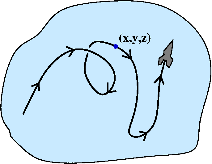 The spaceship in a nebula
My online dictionary states that a nebula is "a cloud of gas
and dust, sometimes glowing and sometimes appearing as a dark
silhouette against other glowing matter." So we could pilot a
spaceship through a nebula. We might be concerned about the physical
effects of the nebula, for example, the temperature. I'll assume that
the spaceship measures temperature at the tip of its front. A point in
the nebula will be located with rectangular coordinates, (x,y,z). The
temperature at that point will be T(x,y,z). The rocket will fly a path
so that at time t its location will be <x(t),y(t),z(t)>.
From this we can see that the temperature measured at the rocket at
time t is T(t)=T(x(t),y(t),z(t)), and this is a composition. First we
find out where the spaceship is at time t, and then we compute the
temperature at that point.
Computing dT/dt
I would like to compute and understand the rate of change of the
temperature, T, with respect to time. It turns out that this is a
significant computation. Now T is a number and t is a number and T is
a function (complication: there are intermediate variables x, y, and
z) of t. So the derivative of T will involve taking its value at
t+Δt and looking for the linearization multiplier. That is what we declared earlier. So here we go. I will
try to accompany the steps of this somewhat elaborate manipulation
with explanations.
|
T(x(t+Δt),y(t+Δt),z(t+Δt))= |
|
|
We are "kicking" the time variable a little bit, and we would like to
examine the change in the T variable. |
|
T(x+x´(t)Δt+H.O.T.,y+y´(t)Δt+H.O.T.,z+z´(t)Δt+H.O.T.)=
|
| |
We use the fact that each of the components of the
position vector are differentiable, so each function value at
t+Δt can be replaced by the original value of the function, a
multiplier (the derivative) which multiplies the disturbance, and
higher order terms. If I were being careful, I would use different
notation for each of the H.O.T.'s, but in practice people don't do
that too often. You'll see why soon. |
|
T(x,y,z)+(∂T/∂x)(x´(t)Δt+H.O.T.)+(∂T/∂y)(y´(t)Δt+H.O.T.)+(∂T/∂z)(z´(t)Δt+H.O.T.)+H.O.T.
|
| | This is the differentiability of T. The
changes in the inputs to T (there are three inputs) are passed
outside. What happens? The linearization idea says that the changes
are each multiplied by an appropriate partial derivative. And this
isn't really exact (the numerical example
showed this!) so there is also a H.O.T. from the
differentiability of T. (Complicated? Sure is.)
|
|
T(x,y,z)+(∂T/∂x)(x´(t)Δt)+(∂T/∂y)(y´(t)Δt)+(∂T/∂z)(z´(t)Δt)+
(∂T/∂x)H.O.T.+
(∂T/∂y)H.O.T.+
(∂T/∂z)H.O.T.+
H.O.T.
|
| | Now I did some multiplication and
rearrangement. I pushed everything involving any of the Higher
Order Terms to the end. |
|
T(x,y,z)+(∂T/∂x)(x´(t)Δt)+(∂T/∂y)(y´(t)Δt)+(∂T/∂z)(z´(t)Δt)+H.O.T.
|
| |
Here is the important step, and it sort of asks you to think a bit
about the ideas of calculus. All of the terms with H.O.T. are
actually, all added together, just another big H.O.T.
|
|
T(x,y,z)+{(∂T/∂x)(x´(t))+(∂T/∂y)(y´(t))+(∂T/∂z)(z´(t))}Δt+H.O.T.
|
| | This is the last rearrangement. Please, I hope
you have the patience to see what has happened. We have the "old"
unperturbed value of T(x(t),y(t),z(t)), and then we have a mess (not
really, as you'll see) multiplying Δt, and then, finally, we
have a whole bunch of things which logically are inside the H.O.T. |
Now what? If f(v) is a function of one variable, then
f(v+Δv)=f(v)+f´(v)Δv+H.O.T.
identifies the derivative of f by what happens to small perturbations.
The red stuff is the derivative, because it is the multiplier of the
small perturbation of the input.
We carried out an elaborate analysis of how the temperature function
changes. Now look at the result again:
T(x(t+Δt),y(t+Δt),z(t+Δt))=T(x,y,z)+{(∂T/∂x)(x´(t))+(∂T/∂y)(y´(t))+(∂T/∂z)(z´(t))}Δt+H.O.T.
The multiplier of Δt is dT/dt, so we see that
|
dT/dt=(∂T/∂x)(x´(t))+(∂T/∂y)(y´(t))+(∂T/∂z)(z´(t))
|
|---|
But this formula is not the point of the discussion. Look at
the equation and think a bit. The
luck and glory is recognizing that the mess on the righthand
side is a dot product. In fact, look:
dT    / ∂T   ∂T    ∂T\    / dx   dy   dz \
-- =   --- , --- , ---  ·   -- , -- , --
dt    \ ∂x   ∂x   ∂x /    \ dt   dt   dt /
Left Right
There are certainly many ways to organize this as a dot product, but
this way turns out to give some insights that amaze me.
Right
The vector on the right-hand side is one we've looked at when
discussing curves. It is the derivative of r(t), the position vector,
so it is v(t), the velocity vector. This vector deals with the
spaceship and its motion.
Left
This vector seems to be "new": it is the vector of
all the first partial derivatives of T in order. This is called the
gradient of T and is frequently written ∇T and is
sometimes also called grad T. The upside-down triangle (or upside
down Δ) is sometimes called "del" or "nabla". This vector can be
computed only from the nebula information.
Thinking about the temperature derivative this way "decouples" (yeah,
a word that's used) the influence of the nebula from that of the
spaceship.
Now I will try to make a sequence of observations which might help people
understand the excitement I feel thinking about gradient.
Observation 1
Let's imagine two spaceship trips through the nebula. Now these
trips (voyages?) may be completely different except that at the
time the two spaceships pass through the point (x,y,z), the
spaceships have the same velocity vectors: that is, the spaceships are
heading in the same direction and at the same speed. Their v(t)'s are
the same. Then the rate of change of the temperature,
dT/dt, that the two spaceships measure is exactly the
same.
I asked students if they could deduce this from the physical and
geometric aspects of the "scenario". I don't think I can. As a math
fact goes, this is nearly obvious: since the v(t)'s are the same, the
right-hand side doesn't change, and the nebula's temperature function
is the same, so the left-hand vector ∇T doesn't change. Therefore
the dot product, which computes dT/dt, is the same. But ... but
... what the heck ... can you "see" this physically? This is not the
temperature at the point, but the rate of change of the
temperature: the rate of change is the same if the velocity vectors
are the same.
Observation 2
Now r´(t)=v(t), the velocity vector. Let me call the unit tangent
vector u(t) here (in the discussion of curvature it was called T(t)
but that will just be too darn confusing). Then v(t) is the same as
(ds/dt)u(t) where ds/dt is the speed and u(t) is the unit tangent
vector. In the formula ∇T·r´(t) the ds/dt effect just
"filters out" of the dot product. If you travel twice as fast on the
same path, then the rate of change of the temperature with respect to
time is just doubled. So this is easy to understand. But the more
subtle aspect is what happens as the direction changes.
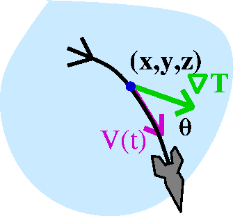 Observation 3
Here I will suppose that ds/dt=1 for simplicity.
Again, call the unit tangent vector, u, for unit
vector. Then what can we say about ∇T·r´(t)? It is
(ds/dt)∇T·u, or just (since I'm assuming unit speed)
∇T·u. But, hey, the dot product is also
||∇T|| ||u||cos(θ). Since cos(θ) is between -1 and +1, I
now know that dT/dt is between -||∇T|| and +||∇T||.
How could we choose u so that dT/dt is largest? We need to make
cos(θ) equal to +1. Therefore we need θ to be 0, and u should
be a unit vector in the direction of ∇T. That is, choose u to be
∇T/||∇T||. To make the rate of change as much negative as possible,
choose u to be -∇T/||∇T||, and then dT/dt will be -||∇T||.
An example (?)
Here is an example.
If T(x,y,z)=x2eyz-5z3 then since
∇T=<∂T/∂x,∂T/∂y,∂T/∂z>, we compute:
∇T=<2xeyz-5z3,x2eyz-5z3(z),x2eyz-5z3(y-15z2)>
As far as I know this function and this computation has no great or special
"meaning".
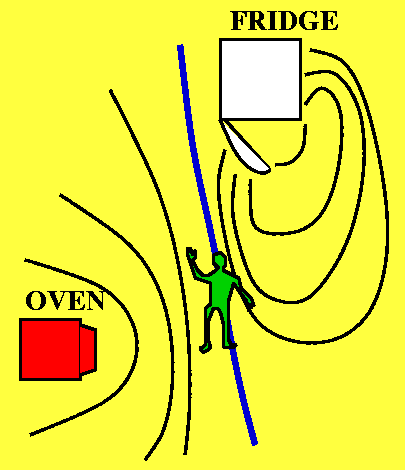 A better example (!)
Im my kitchen I have just finished backing my famous chocolate brownie
pie and I left the oven door slightly open. Also I managed to forget
to close the refrigerator. As a result, the contour lines of
temperature could like what is shown to the right. In what direction
should I go (I am the little green man in the picture!) to most
rapidly increase the temperature? In the direction of the gradient,
which will point towards the oven. I will most rapidly decrease the
temperature by traveling in the opposite direction, towards the source
of the cold.
Observation 4
I could imagine that spaceship travels through the nebula on an
isothermal surface. An isothermal is a collection of points
where the temperature is all the same. We have seen this already:
T(x,y,z)=C is a level surface (dimension 3) or level curve (dimension
2) or a contour {surface|curve}. But if the spaceship travels on such
a surface, then the rate of change of the temperature must be 0. But
then ∇T·v=0. This means that the velocity vector is perpendicular
to the gradient. But then in turn this means that the gradient vector
is perpendicular to the level surface, and it is perpendicular to the
tangent plane of the level surface. In the kitchen, I would walk
perpendicular to the contour lines to increase or decrease
temperature most rapidly. I would walk along the contour lines if I
wanted no rate of change of temperature.
Back to the example
Let me look more closely at the example with
T(x,y,z)=x2eyz-5z3
when x=3 and y=2 and z=1. Well, T(3,2,1)=9e-3. And
∇T=<2xeyz-5z3,x2eyz-5z3(z),x2eyz-5z3(y-15z2)>
becomes
∇T(3,2,1)=<6e-3,9e-3(1),9e-3(-13)>=<6e-3,9e-3(z),-117e-3>
Now forget all that, and solve the following
geometric problem:
What is the equation of a line tangent to the surface
x2eyz-5z3=9e-3 at the
point (3,2,1)?
This could be, indeed, I claim, this is a hard problem. But if
we now disobey my urging ("forget all that") I can tell you that
∇T(3,2,1) is perpendicular to the surface and to its tangent plane
at (3,2,1). So I can write the answer, since I know a point and a
normal vector to the plane requested:
6e-3(x-3)+9e-3(y-2)+-117e-3(z-1)=0.
I think that solving such a problem so efficiently is really remarkable.
Topographic maps
A topographic map shows contour lines. Frequently while hiking people
mind want to find the most direct route to the "top" (a mountain peak)
or to the "bottom" (a creek?). They know by experience that the most
direct route, only looking at the map, that is, only the geometry of
the situation, would be to walk as nearly as possibly perpendicular to
the contour lines.
This can be adapted into computational strategies for finding
maxes and mins. If you can readily compute your function's gradient,
then find maximums by going in the direction of the gradient. This is
hill climbing. Find minimums by going opposite the direction of
the gradient. This is the method of steepest descent. Of course
these computational ideas don't always work, and there are many
implementation details to worry about, but the general strategy is
valuable.
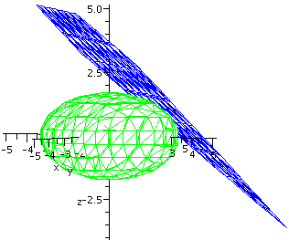 Ellipsoid
Here's a neater example. Consider the ellipsoid (egg)
x2+2y2+3z2=9. The point
(2,1,1) is on this ellipsoid. What is the equation of a plane tangent
to the ellipsoid at (2,1,1)? Well, the gradient of the function
x2+2y2+3z2 is
<2x,4y,6z> and at (2,1,1) this is <4,4,6>. The equation of
the tangent plane is 4(x-2)+4(y-1)+6(z-1)=0.
To the right is a Maple picture made by
the commands which
follow. I hope that the picture helps to convince you that the plane
is the tangent plane. A:=implicitplot3d(x^2+2*y^2+3*z^2=9,x=-5..5,y=-5..5,z=-5..5,grid=[20,20,20],
axes=normal,labels=[x,y,z],color=green,style=hidden);
B:=implicitplot3d(4*(x-2)_4*(y-1)+6*(z-1)=0,x=-5..5,y=-5..5,z=-5..5,axes=normal,
labels=[x,y,z],color=green,style=hidden);
display({A,B};
|
Contour map example
This kind of came up spontaneously in class (I try to have a
well-prepared, well-thought-out lecture, but sometimes things come
up). So to the right is a made-up example of a contour map. The lines
shown are at height multiplies of 100 feet. I hope that you can
see (?) there is sort of one part of the map which deserves the
name "peak" (in the upper left-hand corner). This map is a bit more
complicated than the one I drew in class. I clain there is also a part
of the map which could be named "the pits" (probably at least two of
them!) and that's inside the two loops at the 300 foot height.
|  |
Hill climbing -- a way to get to the maximum
Now suppose we are at the point P on the
map. How should we hike in order to get uphill as fast as possible? I
claim that the directions shown will do that. Notice that I am
not always walking towards "the peak", but I just want to
always walk perpendicular to the contour lines -- in the direction of
the gradient of the height function.
|  |
The method of steepest descent -- how to get to the minimum
This is a way people use to try to get to minima of functions in
several variables. We start at the point Q and
move in the direction opposite the gradient of the height function. In
what I'm showing here, we take some sort of fixed step size (more
sophisticated versions vary the step size) and after that step we keep
going until we hit another contour line. Then we recompute the
direction (minus the gradient) and step again. You can see, I hope,
that this path is headed for one of "the pits".
These methods don't always work and don't always work efficiently, but
they are easy to understand, they can be done in many dimensions, and
the programs run fast.
|  |
The most change
I could also ask where there is the most change in
height in a fixed distance. These are contour lines
corresponding to equal changes in height. The heights will change most
rapidly (as a function of the position on the map) when the contour
lines are most closely spaced. This also corresponds, of course, to
the region in the plane where ||∇ height|| is largest: the
largest magnitude of the gradient vector. I think the region indicated
(in magenta) is the region in this rather simple contour chart.
|  |
I forgot to mention this definition. Please forgive
me!
Directional derivative
If u is a unit vector, then the directional derivative of T at (x,y,z)
in the direction u is the rate of change of T at unit speed in the
direction u (at the point). The textbook's notation for this is
DuT(x,y,z) and the preceding discussion should convince you
that the directional derivative's value is ∇T(x,y,z)·u.
more notation, more words ... this is so
terrific!!! (so academic)
I started a discussion of the more general Chain Rule which I'll
continue next time.
Maintained by
greenfie@math.rutgers.edu and last modified 10/8/2008.
 Suppose I have two copies of the plane, R2. The left-hand
copy in my pictures will have coordinates labeled with u and v and
will be called the uv plane, and the right-hand copy will have
coordinates labeled with x and y and will be called the xy plane.
In this example, x and y will be related to u and v using the
equations
 Now consider a more intricate shape in the uv plane, the unit circle
centered at the origin: u2+v2=1. What shape
corresponds to this circle in the xy plane? Well, since 2u=x, we know
u=x/2, and v=y, so that u2+v2=1 corresponds to
(x/2)2+y2=1.
 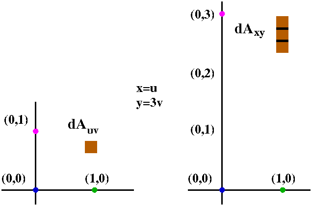 Here is a different relationship between two copies of the plane. In
this example, x and y will be related to u and v using the
equations
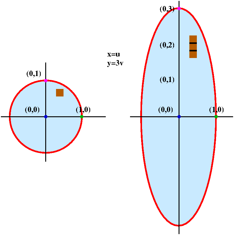
 x=u+5v
 The theorem
 Compute
∫∫R(x-y)40(x+y)50dA where R is
the rectangular region with corners (1,-1), (2,0), (0,2), and (-1,1).
This is an irritating integral. But there is some not well concealed
symmetry. The boundaries of rectangle can be written as x+y=2,
x+y=0, x-y=-2, and x-y=2.
  JAC is the absolute value, 1/2.
 Another example, but this one more realistic
 The planes x=0 and y=0 and z=0 divide R3 into eight
chunks. Differently put, if you remove these planes from space, you'll have
eight pieces left. Each of the eight pieces is characterized by
requiring that the variables x, y, and z have specific (non-zero!)
signs. Ms. Jain asked how the spherical
coordinates φ and θ relate to these sign restrictions.
 θ does not affect the sign of z at all. It interacts with the
signs of x and y. So we can just look "downwards" in R3
from high up on the positive z axis. Then we might understand what
we're seeing as something like usual polar coordinates (remember, the
z information is carried by φ so we don't need that here).
Certainly we can just read off the sign combinations of x and y by the
usual quadrant information of θ.
 Cylindrical coordinates
 z=7r gives a right circular cone whose axis of symmetry is the
z-axis. How can you "see" this? Well, if we restrict ourselves to the
slice of this surface through the xz-plane (with y=0) we get a picture
sort of like what is shown. Why? Because if
y=0, r=sqrt(x2+y2)=x (at least for x>0), so
the result is the line shown.


 FH's latitude is 40.50411oN
and FH's longitude is 74.44836oW.


 Let's let f(x,y)=x2+y2. That's certainly a
simple enough function, just a degree 2 polynomial in x and y.
 dA in polar coordinates
 The plate: from description to integral
 The vertical component of the force is the magnitude of the force
multiplied by the cosine of the angle, φ, between the vertical
line and the line connecting the external object to dA. But cos(φ)
is D/d, which is
D/sqrt(D2+x2+y2). The function to be
integrated is the vertical component of the gravitational attraction
between the external object and dA. This is
GmρD dA/(D2+x2+y2)3/2. Since
the plate is infinite, we want
∫∫All of R2Gmρ dA/(D2+x2+y2)3/2.
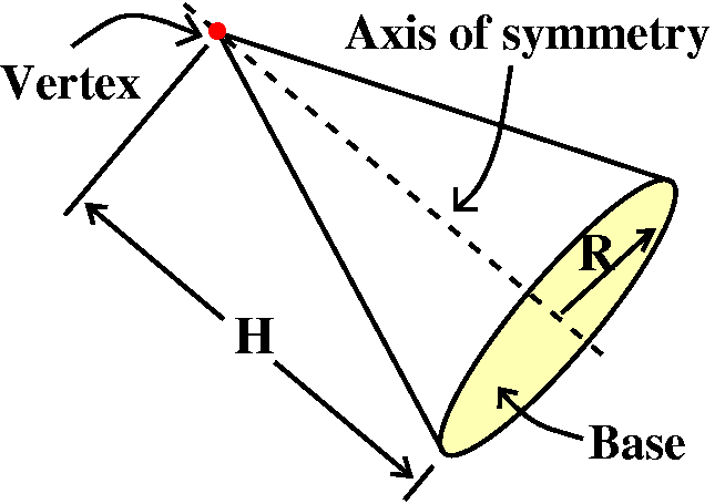 (Almost a real problem!) Moment of inertia of a cone
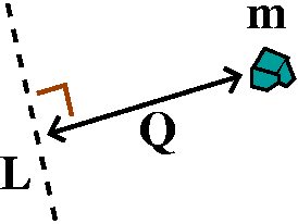
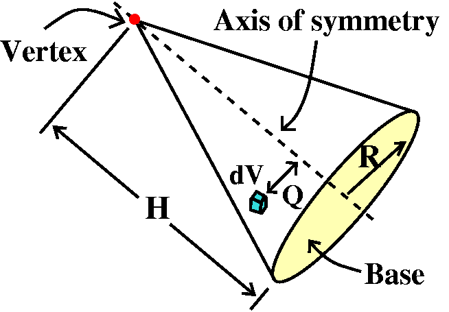 Beginning the analysis
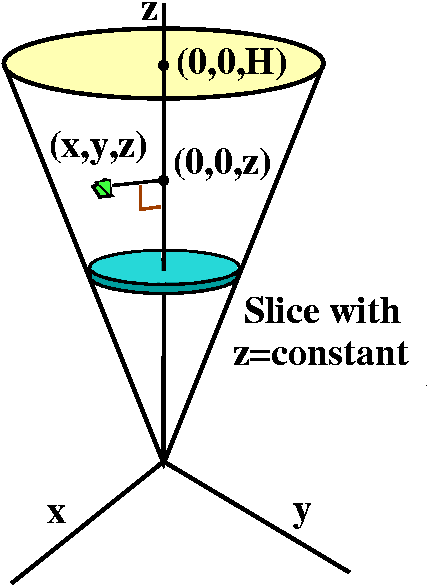 Coordinates?
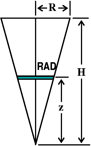
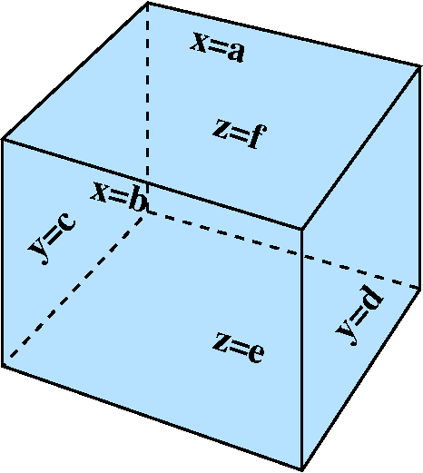 The average temperature of a box of ocean
 Just consider part of this, the fraction
(b-a)(d-c)(f-e)/n3. This is the same as
[(b-a)/n]·[(d-c)/n]·[(f-e)/n]. If n is large, this is
the same as splitting up each of the edges of the box into n equal
pieces, and what we have is a very small box of the ocean. Now if we
also want the points we measure to be well-distributed, then we might
expect that most of the boxes will contain exactly one sample point. We can think of
Temperature at that sample point)·[(b-a)/n]·[(d-c)/n]·[(f-e)/n]
as T(that sample point)dx dy dz or as
T(that sample point)dV where dV is this very small box
inside the huge box of ocean. When we take the SUM we actually have an approximating Riemann
sum to ∫∫∫box of oceanT(x,y,z) dV, which is a
triple integral. Whew! The limit of such approximating sums is the
triple integral, but I won't go into detail because this all parallels
a similar discussion for double integrals. I don't want to forget
anything: there is a factor of (b-a)(d-c)(f-e) remaining on the
bottom, and this is the volume of the box.
  I want to
begin by sketching the region. The planes y=0 (the xz-plane) and z=3
(push the xy-pane up three units) are easy enough. The surface
z=x2+y cut by y=0 and z=3 is maybe not so obvious. When y=0
we get a parabolic arc cut off at z=3 in the xz-plane. As y increases,
the parabolic arc is translated up, but still cut off at z=3. In the
yz-plane, when x=0, the slice is a segment of the line z=y from (0,0)
(with the coordinates being y and z) to (3,3). The surface cuts the
plane z=3 with the parabola 3=x2+y or y=3-x2,
which opens "downward" (in the standard orientation of
xy-planes).
  Nomenclature The surface z=x2+y is called a
tilted parabolic cylinder. It is a parabolic cylinder because
it results from a family of parallel lines in space which all meet the
parabola z=x2 in the xz-plane. It is "tilted" because these
lines are not perpendicular to the xz-plane.

 Now let's try slicing the region by z=CONSTANT, where the
CONSTANT is some unknown number between 0 and 3. This horizontal slice
of the original spatial region gets us something in the xy-plane. If
you were in class, you may recall that there was some effort involved
in sketching the slices that are shown here. But one boundary of the
sliced region is y=0, along the x-axis. The other, curved boundary, is
"inherited" from z=x2+y. Now z=CONSTANT so as a
curve in the xy-plane, if we write it in the standard
y=function of x format, we get
y=z-x2. Therefore this is a parabola (the square on x!)
opening down (the minus sign). The top of the parabola (the vertex)
occurs when x=0, and there y=z. The intersection(s) of the parabola
with the x axis occur when y=0, and there 0=z-x2, so that
x=+/-sqrt(z). The inner double integral is ∫∫
SQUIRREL dx dy. What are the bounds on the
dy integral? We must look at the slice, and see what the highest and lowest values of y are on the slice. The lowest value is 0 and highest value is z: but on the slice, z is a CONSTANT. The highest value depends on z. Now we know:
∫y=0y=z∫
SQUIRREL dx dy

 Volume of a tetrahedron
 In one variable calculus, as I explained last time, the initial
glimpse at the theory in back of the definite integral assumes that
the function doesn't have any jumps. But real functions can
jump! The functions which are met in mechanical engineering (just hit
something!) can certainly look like what's shown to the right. And
similarly, functions met in digital signal processing really can look
like that also. They certainly can be integrated. The secret is that
the jumps really don't matter very much. They can be put inside little
boxes where the variation doesn't matter very much (the red boxes in the picture). So the sums defining the
definite integral still approach a limit, the "correct" limit.
 Converting to iterated integrals
 The other iterated integral
 Now for the dx dy integral. The highest and lowest values for y
are 0 and 9. Therefore the integral must be:
 Integrating Frog over a region

 Suppose we have a nice function f(x) of one variable defined on and
interval, [a,b]. We might want to find the area under y=f(x) on that
interval, althogh that is more of an excuse to define the definite
integral than a real ambition. Here is one approach to the
definition. Take a large positive integer n and divide [a,b] into n
equal parts each of width
 Maybe this is a more realistic "scenario". Suppose you are given a
thin rectangular metal plate with an unknown density
distribution. Therefore this is not necessarily a homogeneous
thin plate. The plate is too heavy or too unwieldy to weigh directly,
and you need to estimate the total mass. Also the mass distribution --
the density -- is not necessarily given by a simple formula. What
maybe could be done is tiny Samples taken at various parts of the
plate, according to some method (maybe depending on accessibility or
expense or ... anything). Then these samples could have their density
measured, and maybe then, after dividing the plate (thoughtwise!) into
pieces, the sample densities could be multiplied by the areas of the
pieces. The sum of these products would then be an estimate for the
mass in the plate. (It is a Riemann sum.) If a better (more accurate?)
estimate was wanted, maybe then use more sample points, smaller areas,
etc. The process is exactly the same mathematics as the definition of
the double integral.
 Maybe all this theory is very nice, but let me show you the way most
double integrals are computed. One method of chopping up a rectangle
is to use vertical and horizontal lines, parallel to the sides. So we
get a grid of subrectangles, each


 Example #1
 Compute the gradients, etc.
Then the multiplier equations and the constraint equation
are:


 Ridiculous interesting (?) fact
 A surface with corners?
 Monkey saddle


 The pictures certainly shouldn't be convincing evidence, but they do
seem to support the assertion that the function has local minimums
at both critical points! (We can verify this assertion with the second
derivative test but this is too much work for me right now.)
Why do I find this disconcerting? Well,
imagine we walk from one peak to another (shown to the right, the
blue "trail"). Shouldn't we somehow pass through a saddle? Well, in
fact, no, we don't need to: maybe the lowest point on the blue trail
is not a critical point -- the tangent plane to the surface at that
point may be tilted. In this example, the tangent plane is
always tilted at every point except the two peaks.
Shouldn't we somehow pass through a saddle?

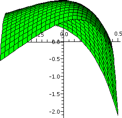
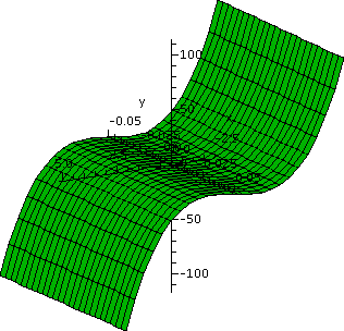
 The situation in 1 variable calculus is considerably different.


 Suppose we have a homogeneous string overlaying part of the x-axis.
The function g(x,t) will represent the following: the height of that
part of the string which is "over" position x at time t. We saw (in
class, in your head: think guitar or violin or rubber band) that
g(x,t) is a function of both x and t. It turns out that under some
very weak assumptions (I am omitting units which multiply things by a
constant) the partial derivatives of the function g(x,t) have the
following strange property:
 and blah means some number between x and x0. Think
of x as close to x0, so blah is close to
x0 also.
Because of the green hypotheses (?) in the
68th derivative test, lots of stuff drops out. In fact, we
know that
f(x)=f(x0)+[f(68)(blah)/68!](x-x0)68. I
bet that if blah is close enough to x0, the sign of
f(68)(blah) is the same as the sign of
f(68)(x0). Well, if the darn sign is positive, then the function sort of looks like
 The spaceship in a nebula
 Observation 3
 A better example (!)
 Ellipsoid