Math 151 diary, fall 2007
In reverse order: the most recent material is first.
Earlier material
Much earlier material
| Tuesday,
December 11 | (Lecture #28) |
|---|
The final exam and related items
Please see this for information
about the final, the TV review, and the review for our lecture. Also
have questions ready for Mr. Yin tomorrow, please!
 Another attempt to foul up ...
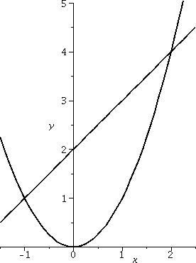
I choose, more or less at random, y=x(x-1)(x-2). I asked people to
sketch this curve, and then attempted to find the (geometric) area
enclosed between the curve and the x-axis. A picture of this is shown
to the right. Sigh. And then we computed two definite integrals,
 01x(x-1)(x-2)dx and
12x(x-1)(x-2)dx. This problem was my attempt
to show that the definite integrals would not balance out. And,
of course, since I made the choice at random, they did balance. Sigh.
01x(x-1)(x-2)dx and
12x(x-1)(x-2)dx. This problem was my attempt
to show that the definite integrals would not balance out. And,
of course, since I made the choice at random, they did balance. Sigh.
The key to the computation of 01x(x-1)(x-2)dx
is the first step, which is multiply out the factors, and get
the standard representation of a polynomial. Integrating that
representation is easy. So
x(x-1)(x-2)=(x2-x)(x-2)=x3-2x2-x2+2x=x3-3x2+2x.
Now we easily can get an
antiderivative: (1/4)x4-x3+x2
and use
FTC 1 to evaluate the definite integrals. So:
01x(x-1)(x-2)dx=(1/4)x4-x3+x2|01=(1/4)-1+1-0=1/4.
12x(x-1)(x-2)dx=(1/4)x4-x3+x2|12=[(1/4)(24)-23+22]-[(1/4)-1+1]=4-8+4-1/4=-1/4.
The total geometric area inside the two bumps is 1/2.
Mr. Louides Ferdinand triumphed
again! There is symmetry here also, and I should have known the two
bumps had the same size.
 Maybe we should have done ...
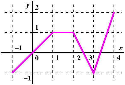
How much geometric area is enclosed by y=x(x-1)(x-3) and the
x-axis? Again, a graph is shown to the right, and these bumps
definitely have different sizes. But my patience
(?) is running out. In a spare tenth of a second, we get:
> int(x*(x-1)*(x-3),x=0..1);
            5/12

> int(x*(x-1)*(x-3),x=1..3);
            -8/3
So the geometric area is 5/12+8/3, which is, I can tell you, 37/12. So
this is 03|x(x-1)(x-3)|dx (the absolute value signs make both bumps "sit" on
top of the x-axis.
Sideways?
I continued my attempt to reach a new level ineptitude by miswriting
the next problem I wanted to analyze. That won't happen here, because
I have the opportunity to think and correct. So I ask,
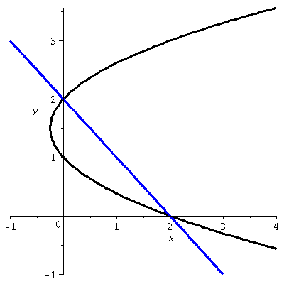
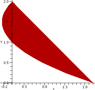
what does the curve defined by the equation (y-1)(y-2)=x look like?
With a bit of thought, we decided that it was a parabola with axis of
symmetry parallel to the x-axis, and that it was opening to the
right. A graph is shown to the right.
Notice, please, that the point (2,0) is on the graph, as well as the
point (0,2). Therefore there's a (exactly one!) straight line through
these two points. Its equation is x+y=2 (Admission: I sort of guessed
at the equation, since the sum of each pair of coordinates is 2, that
must be the equation!). What's the area of the region bounded by the
line and the parabola?
 The dy method
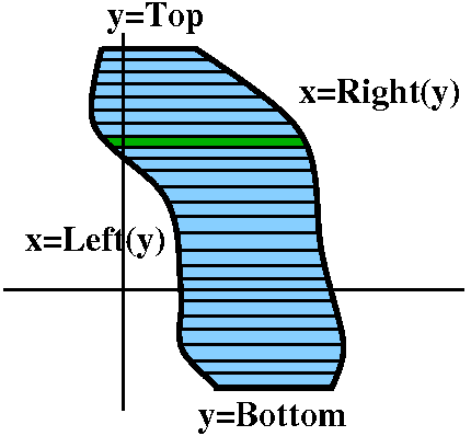
If we have a region in the plane bounded by two curves, x=Left(y) and
x=Right(y) (where Left(y)<Right(y) for the y's of interest here)
and also bounded by lines y=Bottom and y=Top, then we could imagine
slicing this area by lots of horizontal lines dy apart. The region
would be divided into lots of pieces, and each piece would
approximately be retangular. The height of the (almost) rectangle
would be dy, and the width would be Right(y)-Left(y). So the area
would be (Right(y)-Left(y))dy. Since this is the area of a slice, we would get
the total area by taking the Sum of
the areas of the slices, from the Bottom to the Top:
y=Bottomy=Top(Right(y)-Left(y))dy.
In our case ...
 Top is 2 and Bottom is 0. Left(y) is (y-1)(y-2)=y2-3y+2
(you should multiply/distribute/expand/foil whatever! before
integrating) and Right(y) is 2-y. Thus the area can be computed by
Top is 2 and Bottom is 0. Left(y) is (y-1)(y-2)=y2-3y+2
(you should multiply/distribute/expand/foil whatever! before
integrating) and Right(y) is 2-y. Thus the area can be computed by
y=Bottomy=Top(Right(y)-Left(y))dy=
y=0y=2([2-y]-[y2-3y+2])dy=
y=0y=2([2y-y2])dy=y2-(1/3)y3|02=4-8/3=4/3.
Comments
Certainly this is not the only method of getting this area. You could
possibly imagine dissecting the area dx, and chopping it up
somehow so the computation could be done. That would be much more
work, I think. Or maybe you just interchange x and y, and then redraw
the graph, and do it dx. That's certainly possible. I just report,
though, that for many students in the class (physics students,
engineering students) many other geometric and physical quantities
will occur (moment of inertia, center of gravity, etc.) which can be
computed more naturally dy, and therefore "chopping
up" regions in this way will be useful.
What was done very wrong ...
We had a bit more time before the official end of the class
meeting. This was the last lecture of the course, and I want to help
students prepare for the final. I believe that students should prepare
for what they want to avoid in the following sense: assume that
whatever type of problem was most difficult will appear on the final
exam. So I looked at the student performance on the two exams we've
had, and decided to discuss the problems which students had done the
worst (in terms of grades).
Exam #1
Problem 6 had the worst results, followed perhaps by problems 4 and 9.
So let's look at a sample problem asking for information similar to
the what was needed for problem 6.
A problem
Suppose that f(x)=x6-5x3+2. Verify that f has a
root, and locate this root in an interval of length 1/2. Explain why
your assertion is correct.
It isn't even immediately clear to me that this f has a root
since the highest order term is x6, and I know that as
x--> and as x-->-, x6 will get large
positive. So I will compute some values of f. Certainly, f(0)=2 is the
easiest value to check. Now if I were doing this on an exam, I would
probably check either f(1) or f(-1). Notice that if we could assume
that students had calculators, the function to be investigated could
be considerably more complicated! Well,
f(-1)=(-1)6-5(-1)3+2=1+5+2=8. This is positive,
just like f(0), so this is no help. But
f(1)=16-5·13+2=-2<0. I bet there's a
root inside the interval [0,1]. I need finer information, so I
compute f(.5), which is 1/26-5/23+2: I think
that the +2 determines the sign, and f(.5)
is positive. So here is my answer to the problem:
and as x-->-, x6 will get large
positive. So I will compute some values of f. Certainly, f(0)=2 is the
easiest value to check. Now if I were doing this on an exam, I would
probably check either f(1) or f(-1). Notice that if we could assume
that students had calculators, the function to be investigated could
be considerably more complicated! Well,
f(-1)=(-1)6-5(-1)3+2=1+5+2=8. This is positive,
just like f(0), so this is no help. But
f(1)=16-5·13+2=-2<0. I bet there's a
root inside the interval [0,1]. I need finer information, so I
compute f(.5), which is 1/26-5/23+2: I think
that the +2 determines the sign, and f(.5)
is positive. So here is my answer to the problem:
Answer f(1)=-2 is negative and
f(1/2)=1/26-5/23+2 is positive. The function is
a polynomial and is continuous on the interval [.5,1]. The
Intermediate Value Theorem applies, and asserts that for at least one
x in the interval, f(x)=0.
If I would grade the answers to such a problem, I would look for
certain indicators: "Intermediate Value Theorem" and "continuous" as
some abstractions, surely, but applied to the specific function under
consideration. I would also look and assure myself that the student
had supplied specific evidence showing that these abstractions
were correctly applied in this case. I would like all of these to be
present.
Problem 9 asked for computations of limits. Problem 4 asked for the
location of what we've since defined to be a critical point. In both
problems, students made serious mistakes in algebra. I urge
people to check their answers and their work. There will be sufficient
time on the final exam for this.
Exam #2
Certainly problems 2 and 8 had the worst results, followed perhaps by
problems 6 (a geometrical question about Newton's method) and 7 (more
limit computations!). Problem 8 asked students to use (and cite!) a
result in the course connecting information about the distance
traveled if some restrictions on velocity are given. This is a problem
about the Mean Value Theorem, which, as I wrote on the guide to
preparing for the final, is one of the two major results in the course
(the other being FTC). Problem 2 was an optimization problem copied
directly from the textbook. So I thought I would do another textbook
problem. This is problem #23 in section 4.6; the test problem was
problem #27.
A problem
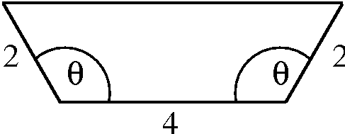 Find the angle
  that maximizes
the area of the trapezoid with a base of 4 and sides of length 2, as
in the figure shown.
that maximizes
the area of the trapezoid with a base of 4 and sides of length 2, as
in the figure shown.
The steps we should follow, as told to me:
Function: area in terms of --> differentiate --> set
equal to 0 --> solve for
I remarked, I pleaded, I requested ... please find out what the
"eligible" 's are first (the
domain that's appropriate for this independent variable in this
problem). Then go on and start the steps listed above. You need to
know what the likely answers should be, and you'll need to know why
you have found a max. All this will be helped greatly if you have the
appropriate domain when you start the steps indicated above.
Diary entry in progress!
| Friday,
December 7 | (Lecture #27) |
|---|
The final exam and related items
Please see this.
Exponential growth: a textbook problem
This is problem #16 of section 5.8: An insect population triples in
size after 5 months. Assuming exponential growth, when will it
quadruple in size?
I added the following question:
What is the doubling time of this type
of insect?
Solution
The phrase "Assuming exponential growth" means that, if B(t) gives
the number of bugs at time t, then we should assume that B(t)=Cekt.
So (units!) B(t) will represent the population of the insects at time t measured in months since the start. We know that B(0)=Ck·0=C and
B(5)=3C. So 3C=Cek·5, and if we divide by C and ln both sides and divide by 5, we get k=ln(3)/5.
So B(t)=Ce[ln(3)/5]t and we want to know when the
population quadruples, that is, reaches 4C. (By the way, it is a good
idea to have some estimate in mind just so we can check the answer,
or, if the answer is correct and way off the estimate, we can improve
estimating skills. In this case, I would guess that about
another month or so is needed to get to four times the initial
population: so my guess is 6, maybe a little bit more.) So let's solve
4C=Ce[ln(3)/5]t: we divide by C, ln both sides, and divide
by [ln(3)/5]. The result is t=[5ln(4)/ln(3)] 6.31 months.
I had also asked "What is the doubling time?" Doubling time is a
standard measure of growth, and is the time needed for the population
to double (indeed!). If the formula governing growth rate is
exponential, then doubling time is a constant (hey, if the population
was given by t2+1, then the population doubles from 0 to 1,
and it also doubles from 1 to sqrt(3): the time intervals change!). In
this case, we are told that population is given by an exponential
formula and that a population quadruples in 6.31 months. I think the
doubling time is 3.15 months.
Exponential decay: a textbook problem
This is problem #16 of section 5.8: A 10-kg quantity of a radioactive
isotope decays to 3 kg after 17 years. Find the decay constant of the
isotope.
I added the following questions:
Also, what's the half-life? What is half-life?
Solution
Well, suppose R(t) is the quantity in kg of the radioactive substance
at time t in years. We assume (and mostly this is true) that amount of
the substance is given by R(t)=Cekt. We know that R(0)=10,
so that C=10 (always try to start the "clock" in these problems at 0
so that C will be the initial amount). Also since R(17)=3,
10ek·17=3. Now divide by 10, ln both sides and
divide by 17: k=ln(3/10)/17. I think this is the decay
constant. Please notice that since 3/10 is less than 1, ln(3/10) is
negative so the constant in the exponential formula is
negative, and this is, indeed, decay.
The half-life of a radioactive substance is the time needed for
an initial quantity to reduce to half. Since we are told that in 17
years, 10 kg reduces to 3 kg, I am sure that a half-life of this
substance will be less than 17. In fact, a half-life will be more
than, say, 8, since a half-life of 8 would result in 2.5 kg at 16. So
a casual estimate of half-life is somewhere between 8 and 17.
Here we want t so that 10e[ln(3/10)/17]t=5. Divide by 10,
take lns, and divide by [ln(3/10)/17]: the result is
t=ln(1/2)/[ln(3/10)/17]. This is about 9.79.
Radioactivity: a very short discussion
There are lots of radioactive isotopes. OA web page I found mentions
these "widely used industrial isotopes ... 192Iridium with
a half-life of 74 days ... and 60Cobalt with a half-life of
5.3 years". If radioactive substances have the same activities (there
are three principal types: alpha and beta particle emissions and gamma
rays) then it is likely that a substance with a shorter half-life will
be more dangerous than one with a longer half-life. But, as Ms. Kravitz reminded me, things can get more
complicated. Please don't think that I know more than a superficial
amount about radioactivity. I also mentioned tritium, which is an
isotope of hydrogen, 3H, widely used to make paint glow
(signs, rifle sights, sometimes as a tracer in the body. It has a
half-life of 12.3 years, although one source I found declared that
when used as part of a biological sample (administered as water) then
the "biological half-life" (a phrase I had not seen before) in humans
was about 10 days (this refers not to the decay of the tritium, which
takes quite a while, but to how a normal human body processes
water). Tritium is not good in the body.
14C
Radiocarbon
dating is one of the most widely used methods of dating human
remains and cultural objects. Please follow the link supplied to read
about it a bit. The basic assumption is that an organic (living)
object has a certain percentage of 14C ("Carbon 14") and
this percent is not replenished which the object is dead. So as the
14C decreases, a reasonable guess about the age of the
object can be made. 14C is convenient because there's a
good amount of carbon in most organic objects, and because the
14C half-life is commensurate (appropriate amount) to
measure much of human history.
One source I found said that the half-life of 14C is about
5,730 years. The text asserts that the decay constant for
14C is about -.000121. Are these two numbers consistent? Is
there some way to check? Well, suppose 14C follows a
Cekt formula. If C=1 and k=-.000121 and t=5,730, then
Cekt should be about a half. In fact, we computed this (or
rather, calculators did) and the result is .499905, which is quite
close to a half. I was happy.
Area between two curves
Here's the final topic of the semester, which is a simple introduction
to the uses of the definite integral. The definite integral has
hundreds of important applications in science and engineering.
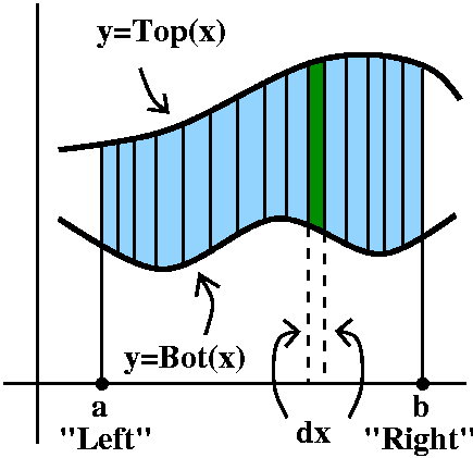
Suppose we are given two functions defined on an interval, Top(x) and
Bot(x) ("Bot" is an abbreviation for "Bottom") and we know on that
interval that Top(x)>Bot(x). How can we compute the area enclosed by the two curves and by vertical lines on the sides of the interval?
I always imagine that the interval is chopped into lots of little
pieces, each of length dx. Then these pieces chop up the area, as
shown in the picture to the right. Each little slice of area is
almost a rectangle (if we ignore the possible tilts at the top
and bottom). The area of the approximate rectangle is [Top(x)-Bot(x)]
(the length of the vertical side, the difference in the heights of the
graphs) multiplied by dx, the width. Now I need to take the Sum of these approximating slices, and add them
up from a to b, or, as I think, from Left to Right. Therefore I believe that the area between these curves on this interval is
LeftRight[Top(x)-Bot(x)]dx.
Random example #1
This example is not random, but it is constructed so I could do it
easily in class. I would like to find the area of the region enclosed
by the line y=x+2 and the parabola y=x2. I would probably
try to begin almost any problem of this type by sketching the region
first. The picture to the left is such a sketch. Where do these curves
intersect? Well, we need to find x's which give the same y, so we
solve x2=x+2 so that x2-x-2=0 and this is (wow!
Oh, hold on, he made it so it would work out) x2-x-2=0 so
that (x-2)(x+1)=0. The roots are x=2 and x=-1.
I honestly think that the phrase "the region enclosed
by the line y=x+2 and the parabola y=x2" specifies exactly
one piece of the plane. You can argue with me -- I discuss this a bit
more in the example below. Here I think we have Left=-1 and Right=2
and Top(x)=x+2 and Bot(x)=x2. So let's compute:
LeftRight[Top(x)-Bot(x)]dx=-12[{x+2}-{x2}]dx=
(1/2)x2+2x-(1/3)x3|-12=[(22/2)+2·2-(8/3)]-[((-1)2/2)+2·(-1)-(-8/3)].
This turns out to be 9/2. I hope. And, by the way, if you look at the
picture, I hope you can see that the region fits inside a box with
height 4 and width 3, so the area should be less than 3·4=12,
which it is. Getting some approximate idea of the answer is useful, if
you, like me, make sign errors and ... well, other kinds of errors.
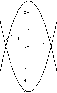 Random example #2
Again, this is an arranged example and everything will work out
neatly. Real problems are rarely like this. I'd like to compute the
area of the part of the plane which is between the parabolas
y=x2-5 and y=3-x2. The first curve opens
up and has its bottom at (5,0). The second opens down, with its
top at (3,0). A picture of the two curves is shown to the right.
I mentioned in class that it is certainly possible to "misunderstand"
the statement of this problem, if you work at it. The plane is
actually divided into five different regions by these two curves. And
maybe someone could maybe declare that there's more than one
candidate for the region between the parabolas (maybe all five
are candidates, or maybe only three of them are?). I guess maybe I
might agree if you really argue with me about it, but if the
discussion is just a way to get out of computing the area of the
only region with finite area
then I would not agree. Please compute the area of that region, and
then, later, argue about it.
The curves intersect where x2-5=3-x2. Since this
is a problem in a math class, let's see: that's 2x2=8 or
x2=4 so that x=+/-2. I think that Left=-2 and Right=+2.
Something new!?
There is a little bit that's new here. Notice that if
Top(x)=3-x2 and Bot(x)=x2-5, then actually
Bot(x) is always negative in the interval [-2,2]. Even so, the
quantity Top(x)-Bot(x) gives the geometric length
of the vertical side of a (dx) thin slice of area. Top(x)-Bot(x) will
be positive. In fact, if you look really carefully at the picture,
you'll see that there are two pieces of [-2,2] where both
Top(x) and Bot(x) are negative. But Top(x) is still bigger than
Bot(x), so Top(x)-Bot(x) will be positive, even though both of them
are negative. The geometric length is still Top(x)-Bot(x).
The computation
LeftRight[Top(x)-Bot(x)]dx=-22[{3-x2}-{x2-5}]dx=
-22[{8-2x2]dx=8x-(2/3)x3|-22=[(8·2)-(2/3)23]-[(8·-2)-(2/3)(-2)3]=64/3.
This is less than a box which is 8 units high and 4 units wide (such a
box would enclose the entire area). Also, several students remarked
that we could have computed the integral from 0 to 2 and doubled the
result, to take advantage of symmetry.
Random example #3
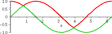
 I would like to find the geometric area between the sine and
cosine curves over one period of these functions. So I drew a
picture similar to what's shown to the right. Again, it may be
possible to misunderstand the question since this situation is more
complicated than previous ones. But "one period" is 2Pi here, and the
word "between" in this situation refers, in fact, to three specific
regions in the picture.
I would like to find the geometric area between the sine and
cosine curves over one period of these functions. So I drew a
picture similar to what's shown to the right. Again, it may be
possible to misunderstand the question since this situation is more
complicated than previous ones. But "one period" is 2Pi here, and the
word "between" in this situation refers, in fact, to three specific
regions in the picture.
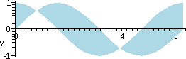 So the area which I wanted to compute is shown to the right. Here is
what I thought that I needed to do (clear evidence that the brain was
not totally functional!). I thought that I would need to split the
area computation into three pieces, and compute three different
integrals, and then add them up. The idea would be as shown to the
left
So the area which I wanted to compute is shown to the right. Here is
what I thought that I needed to do (clear evidence that the brain was
not totally functional!). I thought that I would need to split the
area computation into three pieces, and compute three different
integrals, and then add them up. The idea would be as shown to the
left
 where first one formula then the other, and then the other again, is
on top. Well, this could be done but it would actually be much more
work than is needed.
where first one formula then the other, and then the other again, is
on top. Well, this could be done but it would actually be much more
work than is needed.
Mr. Louides Ferdinand kindly pointed
out that the left-most region and the right-most region when put
together are congruent to the central region: so the sum of the areas
of these two regions must be equal to the area of the region in the
middle. Thank you, Mr. Ferdinand! (Next time I'll get a non-symmetric
example, darn it!)
The curves intersect where sin(x)=cos(x). This is at x=Pi/4 and
x=5Pi/4. So Left=Pi/4 and Right=Pi/4 and between these numbers, the
sine curve will be Top(x) and the cosine curve will be Bot(x). So I
need to compute twice the definite integral over this interval
to get the total area requested. Here we go (and be careful with minus
signs!):
2Pi/45Pi/4(sin(x)-cos(x))dx=-cos(x)-sin(x)|Pi/45Pi/4=[-cos(5Pi/4)-sin(5Pi/4)]-[-cos(Pi/4)-sin(Pi/4)]=
[-{-sqrt(2)/2}-{-sqrt(2)/2}]-[-{sqrt(2)/2}-{sqrt{2}/2}]=4sqrt(2)
There were only SEVEN minus signs
in the next-to-last expression. Mistakes are easy!
| Tuesday,
December 4 | (Lecture #26) |
|---|
Antiderivatives of complicated functions can now (maybe!) be done by
machine. But people can sometimes still do things by hand which complicated
programs may not be able to handle (see below!). People have millions
of years of pattern recognition in their brains. In all of the
examples we did in class, I kept repeating that attention to details
was important, that inserting parentheses was important to help
yourself, that ... well, just be careful!
01sqrt(5x+4)dx
I always try to substitute for the center of the difficulty first
(this does not always work, but it helps in lots of examples). In
this example I would try u=5x+4. So then du=5dx so (1/5)du=dx, and, as
an antiderivative (let me leave out the limits right now):
sqrt(5x+4)dx=sqrt(u)(1/5)du=(1/5)u1/2du=(1/5)(2/3)u3/2+C=(2/15)u3/2+C
=(2/15)(5x+4)3/2+C
The outline of this computation is: from x-land to u-land,
antidifferentiate, back to x-land. Now if we really want to compute
the definite integral, look:
(2/15)(5x+4)3/2|01=(2/15)(93/2)-(2/15)(43/2)
Please notice that the x=0 limit does contribute to this
answer -- you can't just ignore it because, golly, x=0. This antiderivative
has a non-zero value at x=0.
My silicon pal does a great job on this (it even cleans up the
fractions and powers!):
> int(sqrt(5*x+4),x=0..1);
                                      38
                                      --
                                      15
x·sqrt(5x+4)dx
As I remarked in class, I think that most people could have made a
good guess at the previous antiderivative. I can't do this one without
a substitution and some subsequent manipulation. So again let us try
the center of the difficulty, u=5x+4, so du=5dx and (1/5)du=dx. But
now to get to u-land we need to know how to translate x. Since u=5x+4,
we know that u-4=5x and (1/5)(u-4)=x. Therefore:
x·sqrt(5x+4)dx=(1/5)(u-4)u1/2(1/5)du [to u-land]
(1/25)(u-1)u1/2du=(1/25)u3/2-u1/2du
[pull out constant multiplier, distribute u powers]
(1/25)((2/5)u5/2-(2/3)u3/2)+C=(1/25)((2/5)(5x+4)5/2-(2/3)(5x+4)3/2)+C [antidifferentiate, and back to x-land. Notice that
1/(5/2)=2/5. etc.].
Although it may be possible to check an antiderivative by
differentiating, you may not want to!
x2sqrt(5x+4)dx
Here I pushed up a power of the x. If you use u=5x+4 again (the
center of the difficulty) then as before, (1/5)du=dx and
(1/5)(u-4)=x. So the integral becomes:
x2sqrt(5x+4)dx=[(1/5)(u-4)]2sqrt(u)(1/5)du
This is not so pleasant but we can do it. Now
[(1/5)(u-4)]2=(1/25)(u2-8u+16) and so:
[(1/5)(u-4)]2sqrt(u)(1/5)du=(1/125)u5/2-8u3/2+16u1/2du
So what did I do there? Well, I squared 1/5 to get 1/25, and then
multiplied by another 1/5 to get 1/125. Multiplicative constants can be
pulled "out" of the indefinite integral. Other kinds of constants
can't! Then I distributed the sqrt(u)=u1/2 over the
other terms. Powers of u can be antidifferentiated easily, so we get:
(1/125)((2/7)u7/2-(16/5)u5/2+(32/3)u3/2)+C
Now back to x-land:
(1/125)((2/7)(5x+4)7/2-(16/5)(5x+4)5/2+(32/3)(5x+4)3/2)+C
I surely would not want to check this by differentiating! My "pal", in
about two-hundredths of a second (.02 seconds) gives this:> int(x^2*sqrt(5*x+4),x);
3/2 2
2 (5 x + 4) (128 - 240 x + 375 x )
-------------------------------------
13125
I hope (I guess!) this is what we have. It sort of looks the same!
|
x·sqrt(5x2+4)dx
Here u=5x2+4 (the most "horrible" thing in the integral),
du=10x dx, (1/10)du=x dx (because notice that there is an x
inside the integral -- not an accident!). From x-land to u-land, then,
we get:
x·sqrt(5x2+4)dx=sqrt(u)(1/10)du=(1/10)u1/2du=(1/10)(2/3)u3/2+C
The x did not just disappear! It was needed in this case to be
part of du. And finally we change (1/10)(2/3)u3/2+C to
(1/10)(2/3)(5x2+4)3/2+C. You can check
this by differentiating, if you use the Chain Rule correctly. The 2/3
cancels the 3/2 coming from the power outside, and the 1/10 cancels
the 10 in the 10x coming from what is inside.
sqrt(1+sqrt(x))dx
I remarked that I could show people how to compute an antiderivative
that commonly used programs would not do. This antiderivative is the
beginning. Here we tried the substitution u=1+sqrt(x), so
du=(1/2)x-1/2dx. If we solve for dx, the result is
dx=2sqrt(x)du, which is 2(u-1)du. So:
sqrt(1+sqrt(x))dx=sqrt(u)2(u-1)du=2u3/2-u1/2du=2((2/5)u5/2-(2/3)u3/2)+C=2((2/5)(1+sqrt(x))5/2-(2/3)(1+sqrt(x))3/2)+C
O.k.: this is good. It is sort of ugly, but it is certainly not the
most complicated computation in the world.
sqrt(1+sqrt(1+sqrt(x)))dx
So let's try the same u as before. Then:
sqrt(1+sqrt(1+sqrt(x)))dx=sqrt(1+sqrt(u))2(u-1)du
If we make another substitution: v=1+sqrt(u), then
dv=(1/2)u-1/2du, so 2u1/2dv=du and
2(v-1)dv=du. So go from u-land to v-land. We also need to know u in
terms of v, but v=1+sqrt(u) leads to (v-1)2=u.
sqrt(1+sqrt(u))2(u-1)du=sqrt(v)2((v-1)2-1)2(v-1)dv
O.k. Let's see what the mess in v-land actually looks like if we
multiply out things (sorry: "expand expressions"):
v1/2)2((v-1)2-1)2(v-1)=4v1/2((v2-2v)(v-1)=4v1/2(v3-3v2+2v)=
4v7/2-12v5/2+8v3/2
The last expression is just a bunch of powers of v, so its
antiderivative is easy. Here it is:
(8/9)v9/2-(24/7)v7/2+(16/5)v5/2+C
Now back to u-land with v=1+sqrt(u):
(8/9)[1+sqrt(u)]9/2-(24/7)[1+sqrt(u)]7/2+(16/5)[1+sqrt(u)]5/2+C
Now back to x-land with u=1+sqrt(x):
(8/9)[1+sqrt(1+sqrt(x))]9/2-(24/7)[1+sqrt((1+sqrt(x)))]7/2+(16/5)[1+sqrt(1+sqrt(x))]5/2+C
There we go!
We've computed an
antiderivative that the
calculators students had in class
couldn't do!
Cheers for the human beings among us, who have
both pattern recognition and patience.
|
sqrt(1+sqrt(1+sqrt(1+sqrt(x))))dx
O.k., I bet if you paid me enough (I'm cheap!) I could find an
antiderivative for this function. The big and powerful program
Maple, available on most Rutgers systems
gives:
> int(sqrt(1+sqrt(1+sqrt(1+sqrt(x)))),x);
                      /
                     |                  1/2 1/2 1/2 1/2
                     |  (1 + (1 + (1 + x   )   )   )    dx
                     |
                    /
This response indicates that the program could not find an
antiderivative in terms of familiar functions.
Mathematica, probably the most widely
known Maple competitor (and also
available on some Rutgers systems) has
an integration
webpage on line. When asked to find the antiderivative of
sqrt(1+sqrt(1+sqrt(1+sqrt(x)))), the response is
Mathematica could not find a formula for your integral. Most likely
this means that no formula exists.
I don't agree. I could do it, just ask (but politely and
persuasively!). I believe people and computers can work together
usefully, each with their strengths.
exsin(5ex+7)dx
Pattern: the worst thing is certainly inside sine. So I will
try u=5ex. Then du=5exdx, and
(1/5)du=exdx. From x-land to u-land, to antidifferentiate,
and back to x-land;
exsin(5ex+7)dx=(1/5)sin(u)du=(1/5)(-cos(u))+C=(1/5)(-cos(5ex+7))+C.
Three ln integrals
I asked groups of students to go to the board and compute three
increasingly difficult (at least to me!) integrals involving ln which
are problems in section 5.7. Here
they are:
- [(ln x)2/x]dx
Solution Take u=ln x (since ln is the center of the difficulty), so du=(1/x)dx, and recognize
please that we have dx/x in the integral! So from x-land to
u-land:
[(ln x)2/x]dx=(ln x)2[dx/x]=u2du
Now integrate and get u3/3+C, which in x-land is
(ln x)3/3+C. Is this good?
- [1/{x·ln x)]dx
Solution Take u=ln x and again du=(1/x)dx. The integral
changes:
[1/{x·ln x)]dx={1/u]du=ln(u)+C=ln(ln(x))+C
This really is not too horrible. People use functions like this one,
really.
- [{ln(ln(x))}/{x·ln(x)}]dx
O.k., this example is more of a textbook example. So, again, I will
try u=ln x and again du=(1/x)dx. We will go from x-land to
u-land:
[{ln(ln(x))}/{x·ln(x)}]dx=[ln(u)/u]du
Please notice that the substitution absorbed (?) one of the things in
the bottom of the integrand. Now what should we do? If you were
"properly conditioned" by the previous examples, you would try a substitution and so I will. What I choose
to try (it works, that's why!) is v=ln(u) and dv=[1/u]du. So from
u-land to v-land:
[{ln(u)/u]du=v dv=(1/2)v2+C
Now back and back again:
(1/2)v2+C=(1/2)(ln(u))2+C=(1/2)(ln(ln(x)))2+C
A differential equation and initial condition again
I'm following the text here. We are next supposed to consider a new
sort of differential equation. We have studied such problems as
these:
y´=3x4+{2/x4} and
y(1)=2.
This is an initial value problem, with a differential equation and an
initial condition. We find what's called the general solution by
computing an antiderivative:
3x4+{2/x4} dx=3x4+2x-4dx=(3/5)x5-(2/3)x-3+C
The perhaps interesting aspects of what was just computed are these: I
first changed {2/x3} to 2x-3, which is a more
standard way to write powers of x. I regard things like sqrt(x) (just
x1/2) and 1/sqrt(x) (surely x-1/2) as
invitations to error, directed personally at me. Unfortunately I
accept these invitations sometimes. Then I antidifferentiated. Making
sure that a minus sign appears in the answer (a consequence of the
transition from -3 to -2) is also something I foul up sometimes. Oh
well. Now onward.
The initial condition y(1)=2 allows us to pick out a particular
solution by finding a value of C in the general solution:
Since y(1)=2, (3/5)15-(2/3)1-3+C=2. This means
(3/5)-(2/3)+C=2 or C=61/15.
The solution is f(x)=(3/5)x5-(2/3)x-3+(61/15).
A different kind of differential equation
We look at dy/dt=ky where k is a constant. The independent variable is
usually called t here instead of x. The reason for t (time)
will become apparent, I hope. Notice that this is a very different
kind of equation, because what's on the right-hand side is a constant
multiplied by y. We can't solve it by just antidifferentiating ky
because we don't know y. So a different approach must be
used. There will be more about such equations in Math 152. This is a
simple example designed to help you work with a number of useful
applications.
Translation into English; what is this?
I asked people to translate the equation dy/dt=ky in English. This is
difficult. Here is a possible candidate for such a translation:
The rate of change of y over time (dy/dt) is directly proportional to
y itself. ("Directly proportional" means that when the amount of y
changes, that the rate of change of y is changed by k mutliplied by
the change.)
This is a terrible "translation". I am sorry. Maybe I'd
better stick with adding fractions. English is too difficult!
There are many real phenomena which satisfy this sort of growth (or
decay) rule. Examples include:
- Bacterial growth (see below for comments on this model).
- Radioactive decay (this is modeled fairly well by this
differential equation).
- Compound interest (technicality: the interest should be compounded
continuously)
- Certain chemical reactions (mostly, sometimes).
- The spread of rumors (really, this is also approximately true:
think about it. If a certain number of people know that, say, Britney
Spears and I are friends then the spread of this "information"
is approximately directly proportion to the number of people who know
this and want to spread the rumonr. As the population gets more
"saturated" with this information, the model begins to be less
accurate.)
What are the solutions?
I would hope that dy/dt=ky would have a family of solutions
(the general solution) and we would use an initial condition to pick
out one of these (the particular solution).
Well, first let's guess one solution of dy/dt=ky. For example,
I know a wonderful function which is its own derivative: the
exponential function (so that's a solution when k=1). After some
further consideration, the function ekt was
suggested. Indeed, if we differentiate this, the Chain Rule "spits
out" a multiplicative factor of k, so the derivative of ekt
is ektk, and this is ky.
Are there other solutions? Here is a trick to learn about other
possible solutions. It is a fairly clever trick, and is used in other
computations, which is why I'm showing it to you. Suppose y is
another solution of dy/dt=ky. I want to compare it to
the solution we know, ekt. The trick is to compare this
way:
Look at y/ekt (the unknown solution y divided by the known
solution, ekt). Let's differentiate this. The Quotient Rule
gives uys:
y´(ekt)-y(ektk)
---------------
(ekt)2
Look carefully at the top of the fraction. We are assuming
that y´ is ky. Then the top becomes:
y´(ekt)-y(ektk)=ky(ekt)-y(ektk)=0
because things exactly cancel. This means (MVT tells us: a function
with 0 derivative is constant) y/ekt is a
constant, C. So y=Cekt.
Cekt
I admit totally truthfully that I don't go through any process
remotely like what I just showed you in practice. In fact, if I think
that the differential equation dy/dt=kt is a good description of a
situation, then I immediately jump to Cekt. If you work
with such situations for a while, I think you will do this also.
Mr. Patel's bacteria
Mr. Nitesh Patel graciously suggested
the following (hypothetical) observations of a bacterial colony:
Initially, there are 50 bacteria. In 3 hours, 100 bacteria are
observed (3 hours is called the doubling time). In 6 hours, 200
bacteria are observed.
People believe that dy/dt=kt is a differential equation which
approproiately describes growth in such a situation (some comments on
this assumption are below!) because bacteria (generally) reproduce
asexually by division, and new bacteria are created by a fraction of
the current bacteria splitting. I would like to make a mathematical
model (in this case, get a simple formula) for the bacteria at time t.
I will measure t in hours from the start of the observation. B(t) will
be the number of bacteria at time t. So B(0)=50 and B(3)=100 and
B(6)=200. If we suppose that B(t)=Cekt (that follows from
the differential equation's applicability to this situation) then we
need to identify numbers for C and k.
Since B(0)=50 and
B(0)=Cek·0=Ce0=C·1=C. So C is
50. Now we know that B(t)=50kt. We need to identify k, and
we can use B(3)=100 for this. So: 100=50ek(3) which is
2=e3k which is (take ln's!) ln(2)=3k so that
k=[ln(2)/3]. (People who work with these equations a great deal
develop lots of computational shortcuts!).
So the number of Mr. Patel's bacteria is given by
B(t)=50e[ln(2)/3]t. We could check this formula by plugging
in t=6, since we know the answer should be 200. Here:
B(6)=50e[ln(2)/3]6=50e2ln(2)=50eln(4)=50·4=200
(because exp and ln are inverse functions).
Defects of the model?
Maybe bacteria don't reproduce the way we think (indeed, when I was
younger, mostly people did believe bacteria could only reproduce
asexually, but this is not always true). There's a more subtle
assumption hidden in the model. The exponential function grows very fast. For example, there will be
1010 bacteria in about 82 hours (I did these computations
secretly). That isn't so big, biologically, since there may be about
1014 cells in the human body. But if you continue to
believe this model is valid, there will be 10100 bacteria
after about five and a half weeks. Now to understand 10100
is difficult. Uh ... there are about, say, 6 billion people in the
world, and so there are about
6·109·1014=6·1023
human cells in the world. Multiplied exponentials add
"upstairs". This means we'd need lots and lots of worlds (more than
1075) to have maybe one bacteria per cell.
In fact, the bacteria will grow exponentially as long as conditions
allow. That is, there needs to be adequate food, places to excrete
poisons, etc. I think, in reality, these limits to growth
impose themselves in a realistic way fairly soon in the case of
bacterial growth. So the exponential model for bacterial growth is
valid, but really only for relatively brief intervals. Exponential
decay (with k<0) can be applied more appropriately over long
periods of time to radioactivity. I'll try to discuss this next time.
| Friday,
November 30 | (Lecture #25) |
|---|
FTC 1
If F´=f, then abf(x) dx=F(x)|ab=F(b)-F(a).
Simple examples
01x1/3dx=(3/4)x4/3|01=(4/3).
Magic? I think it is very easy to not think about even "simple"
computations like evaluating this integral. If we used Riemann sums, I
believe getting an exact answer would require quite a bit of
manipulation. Here all we need to do is guess (?) an
antiderivative of x1/3 (hey, it comes from a power one unit
higher, well, then we need to correct for the number that comes down
in front, so the answer should be ...) and then the number practically
presents itself. This is amazing technology to me.
49(3x2-1/sqrt(x))2dx. There are various approaches which are
possible. The simplest which occurs to me is just to expand the
square. That is:
(3x2-1/sqrt(x))2=(3x2)2+2·(3x2)·(-1/sqrt(x))+(-1/sqrt(x))2=9x4-6x3/2+1/x.
So now we compute 499x4-6x3/2+1/x dx=
(9/5)x5-6(2/5)x5/2+ln(x)|49=(9/5)95-6(2/5)95/2+ln(9)-(=(9/5)45-6(2/5)45/2+ln(4)). I would be content with this answer on an
exam. Also, please note the big parentheses. I tell you with true
humility that I have messed up such parentheses too many times. They
are easy to forget.
015ex+2e-xdx. Here
the challenge in applying FTC 1 is getting an
antiderivative. Well, ex is its own antiderivative. What
about an antiderivative of e-x? First, I would "guess"
e-x. But then I would quickly check and correct. That is,
if we d/dx e-x, the result would be -e-x, so a
suitable antiderivative would be -e-x. Now look:
015ex+2e-xdx=5ex-4e-x|01=
5e1-4e-1 -(5e0-4e-0)=5e-4/e-1.
FTC 2
If F(x)=axf(t) dt, then F´(x)=f(x).
An alphabet lesson
What is 01x2dx? In the last lecture,
we saw with several different techniques that this is 1/3. Then let's
play a little logical game.
- What is the value of 01x2dx? The value is 1/3.
- What is the value of 01w2dw? The value is 1/3.
- What is the value of 01t2dt? The value is 1/3.
- What is the value of 012d? The
value is 1/3.
- What is the value of 01
 2d? The
value is 1/3.
2d? The
value is 1/3.
The labels d(something) inside the definite integral do not get
"communicated" to the outside. This is just like the index of
summation in one of those  's. This is the analogue of what is called a local
variable in computer science, defined inside a for loop or a
subprogram or subroutine. In math, one phrase used for such a thing is
local variable. The letter is there to help the computation,
but only has a meaning within the scope of the computation of the
integral.
's. This is the analogue of what is called a local
variable in computer science, defined inside a for loop or a
subprogram or subroutine. In math, one phrase used for such a thing is
local variable. The letter is there to help the computation,
but only has a meaning within the scope of the computation of the
integral.
Simple example
Describe a function whose derivative is cos(x+ex).
This is either very very easy, or, for reasons that will be discussed
more in Math 152, very very hard. I will give the very very easy
answer here.
One function is F(x)=-3xcos(t+et) dt.
This is a function whose derivative is
cos(sqrt(x)+ex) by using FTC 2.
Another function is G(x)=5xcos(w+ew) dw.
Let me compare the two answers. One has inside variable t and the
other has inside variable w. This doesn't matter. They both are
"satisfactory" answers to the question asked because FTC 2 implies
that the derivative of a definite integral with a variable upper
parameter is the integrand's value at that upper parameter (hey, I'm
using all of the high-priced words!) One answer is a definite integral
from -3 to x and the other is a definite integral from 5 to x. Using
property (*) from last time, the two answers are different by this:
-35cos(s+es) ds. What
is this? It is a constant (I'm just using another variable, s, to
again bring up the idea of a "dummy variable"). Two functions which
differ by a constant have the same derivative. So that's o.k.
 By the way, it can be proved that no one can do much better in
this problem than write the answer as a definite integral. There isn't
any much simpler answer. Software can then plot this function, because
people have spent a great deal of time and effort learning how to
compute good numerical approximations to definite integrals very
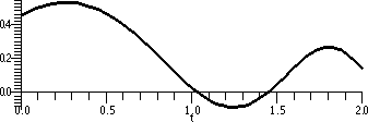
rapidly. The picture of F(x), the antiderivative of
cos(x+ex) which is defined above, on the interval [0,2] was
produced by Maple in less than
three-tenths of a second. I am sure other software would do the job as
well.
By the way, it can be proved that no one can do much better in
this problem than write the answer as a definite integral. There isn't
any much simpler answer. Software can then plot this function, because
people have spent a great deal of time and effort learning how to
compute good numerical approximations to definite integrals very
rapidly. The picture of F(x), the antiderivative of
cos(x+ex) which is defined above, on the interval [0,2] was
produced by Maple in less than
three-tenths of a second. I am sure other software would do the job as
well.
More examples (a textbook problem)
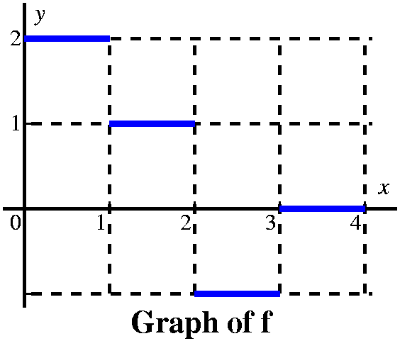 This is problem 23 in section 5.4. The graph of f is given to the
right. The problem asks us to sketch a graph of
A(x)=0xf(t) dt. I presume, since f's
graph is given on the interval [0,4], that we are supposed to sketch a
graph of A(x) on the same interval.
This is problem 23 in section 5.4. The graph of f is given to the
right. The problem asks us to sketch a graph of
A(x)=0xf(t) dt. I presume, since f's
graph is given on the interval [0,4], that we are supposed to sketch a
graph of A(x) on the same interval.
There are various strategies for analyzing this sort of problem. Since the
information is furnished graphically, I'd probably try to do the
problem graphically, or at least begin it that way. I would think of
the limits, 0 and x, and try to see how the definite integral (which
I'd think of as signed area) varied as x varied.
|
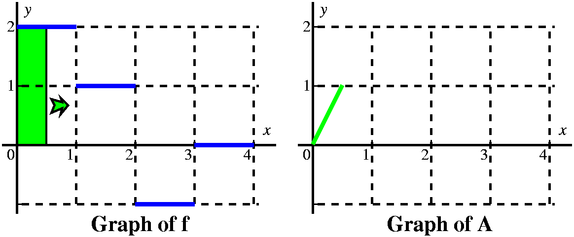 Let's consider first x's between 0 and 1. Here I think
of a vertical line somewhere over the [0,1] interval, moving to the
right. The area between that line and the y-axis, under y=2, is
0xf(t) dt. Since the line has height 2,
the area is 2x, and the graph of A is a straight line segment starting
from (0,0) with slope 2.
Let's consider first x's between 0 and 1. Here I think
of a vertical line somewhere over the [0,1] interval, moving to the
right. The area between that line and the y-axis, under y=2, is
0xf(t) dt. Since the line has height 2,
the area is 2x, and the graph of A is a straight line segment starting
from (0,0) with slope 2.
|
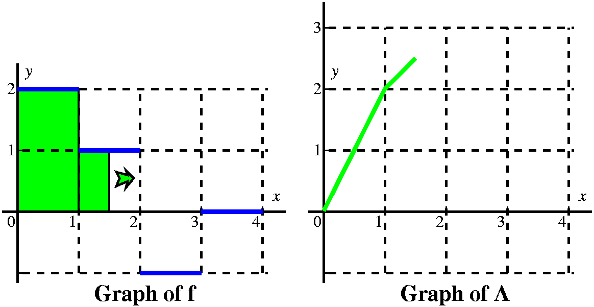 When the vertical line passes x=1, we have accumulated 2 units of
area, and A(1)=2. But now the "profile curve", f, changes height. It
has height 1. We must add to the 2 units of accumulated area the new
area we are getting between x and 1. Since the height of f is 1, and
the base is x-1, we are add on 1(x-1) units of area.
When the vertical line passes x=1, we have accumulated 2 units of
area, and A(1)=2. But now the "profile curve", f, changes height. It
has height 1. We must add to the 2 units of accumulated area the new
area we are getting between x and 1. Since the height of f is 1, and
the base is x-1, we are add on 1(x-1) units of area.
The graph of A in this interval will be linear with a slope of 1, and
it will start from (2,2).
|
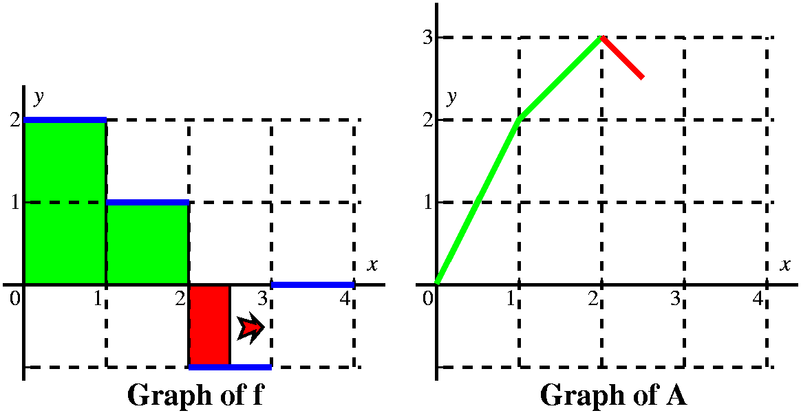 At x=2, we have accumulated 3 units of area, 2 over the interval
[0,1], and 1 more over the interval [1,2]. Now x moves to the right in
the interval [2,3]. The height of f is -1, so the definite
integral will decrease: the geometric area is below the
x-axis. We know A(2)=3 becuase of the accumulated area.
At x=2, we have accumulated 3 units of area, 2 over the interval
[0,1], and 1 more over the interval [1,2]. Now x moves to the right in
the interval [2,3]. The height of f is -1, so the definite
integral will decrease: the geometric area is below the
x-axis. We know A(2)=3 becuase of the accumulated area.
But if x is between 2 and 3, the change in A is (-1)(x-2). So we need
to show the graph of A decreasing, and it will be decreasing linearly
in x, with a slope of -1.
|
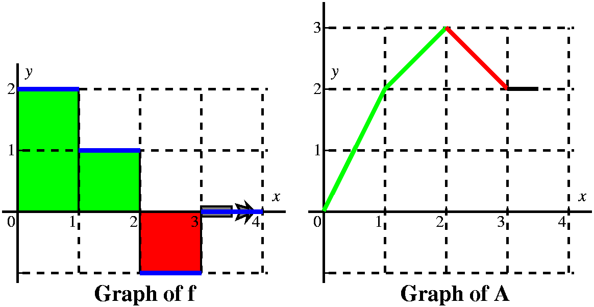 By the time the vertical line has gotten to x=3, it has accumulated
3-1 units of area. Yes, I know that 3-1=2, so actually A(3)=2,
but somehow writing and thinking 3-1 helps me recall that + is assigned to areas above the x-axis and
– is assigned to areas below the x-axis.
By the time the vertical line has gotten to x=3, it has accumulated
3-1 units of area. Yes, I know that 3-1=2, so actually A(3)=2,
but somehow writing and thinking 3-1 helps me recall that + is assigned to areas above the x-axis and
– is assigned to areas below the x-axis.
Between 3 and 4, the height of f is 0 (zero: nothing). There is
therefore no change in the area as we move the upper limit on the
definite intergral to the right. And therefore there is no change in
A, and the graph of A is a horizontal line segment beginning at (3,2).
|
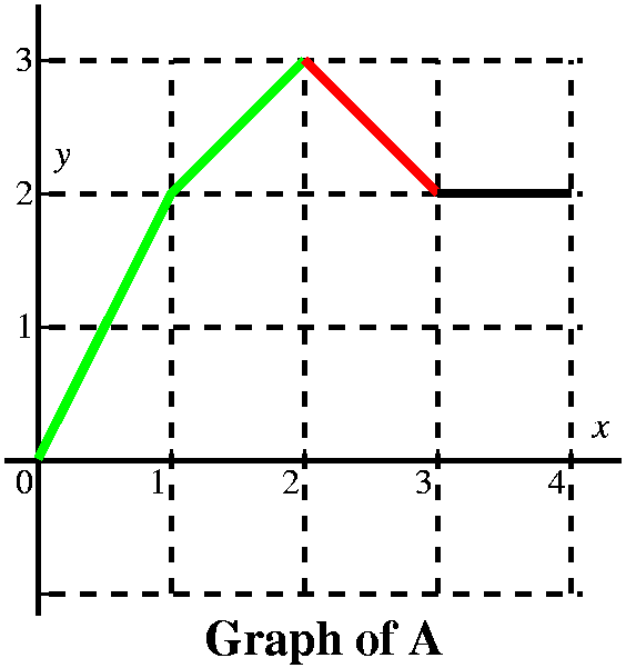 From this we get a very good idea of the graph of A(x). It is 4 line
segments with slopes of 2, 1, -1, and 0. It is a continuous function.
The slopes of A correspond to the heights of f, and actually A is an
antiderivative of f (the antiderivative with the initial condition
A(0)=0), so f is the derivative of A. I think the graph looks like
what's shown to the right.
From this we get a very good idea of the graph of A(x). It is 4 line
segments with slopes of 2, 1, -1, and 0. It is a continuous function.
The slopes of A correspond to the heights of f, and actually A is an
antiderivative of f (the antiderivative with the initial condition
A(0)=0), so f is the derivative of A. I think the graph looks like
what's shown to the right.
|
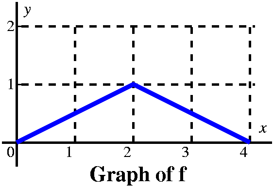
Part B
 Well, there's actually a part B) to this problem. The graph to the
right is given, and, again, we are asked to graph
A(x)=0xf(t) dt. Here the graph is a bit
more complicated (well, it is more complicated to me: the other
function had exactly 4 values, and this function has lots and lots of
values!).
Well, there's actually a part B) to this problem. The graph to the
right is given, and, again, we are asked to graph
A(x)=0xf(t) dt. Here the graph is a bit
more complicated (well, it is more complicated to me: the other
function had exactly 4 values, and this function has lots and lots of
values!).
I'll use a strategy different from what we did in A) to
understand and solve this problem.
|
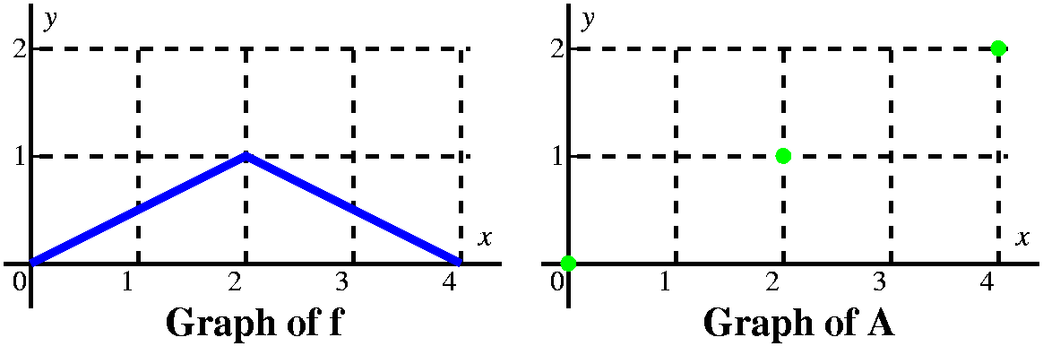 Probably I would look at the graph and learn that A(0)=0 (there is
no area from 0 to 0!). I would look a bit more and find that
A(2)=1, because 02f(t) dt is the area of
a triangle with base 2 and height 1, and (1/2)(2)(1)=1. Finally, I
would see that A(4)=2, because there are two of those triangles. So I
have the three dots shown to the right on the graph of A.
Probably I would look at the graph and learn that A(0)=0 (there is
no area from 0 to 0!). I would look a bit more and find that
A(2)=1, because 02f(t) dt is the area of
a triangle with base 2 and height 1, and (1/2)(2)(1)=1. Finally, I
would see that A(4)=2, because there are two of those triangles. So I
have the three dots shown to the right on the graph of A.
Notice also that the graph of A is increasing because as we
move the right limit to the right we are getting more and more area,
and this is positive area since it is above the x-axis.
|
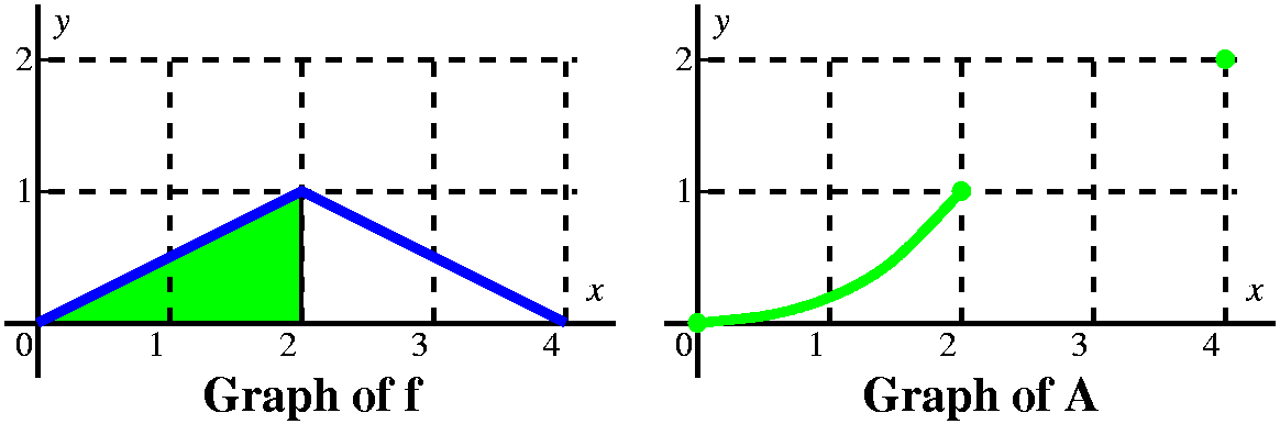 What can we say about the derivative of A in the interval [0,2]? By
FTC 2, this derivative is the function f, and the function f is just
(1/2)x. That means the second derivative of A is 1/2, and this is
positive. So the graph of A between 0 and 2 is concave up, and
connects (0,0) and (2,1).
What can we say about the derivative of A in the interval [0,2]? By
FTC 2, this derivative is the function f, and the function f is just
(1/2)x. That means the second derivative of A is 1/2, and this is
positive. So the graph of A between 0 and 2 is concave up, and
connects (0,0) and (2,1).
I actually know a formula for A, since A(0)=0 and
A´(x)=(1/2)x. It must be (I antidifferentiate and get the correct
constant!) A(x)=(1/4)x2. So what I see between 0 and 2 is a
piece of a parabola.
|
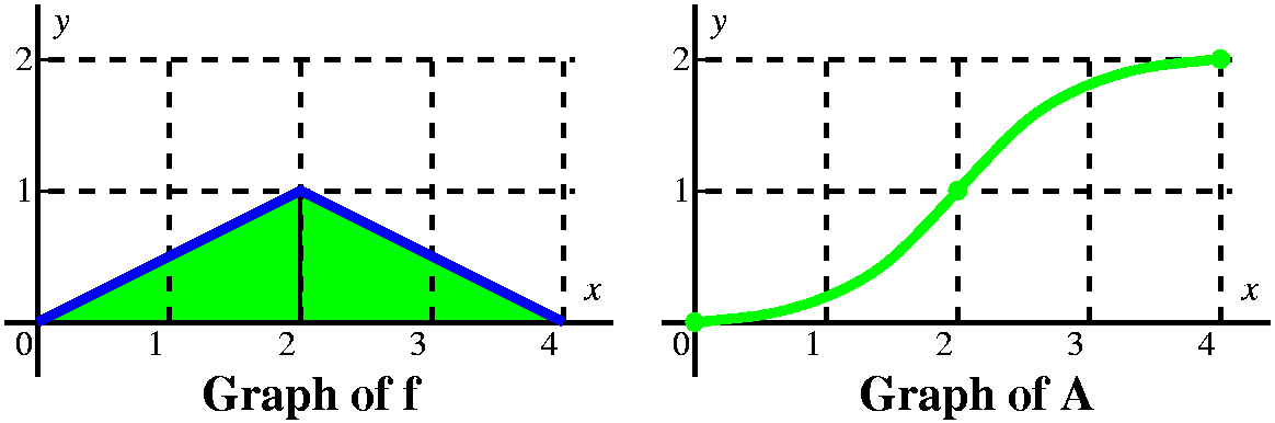 Between 2 and 4, the function keeps increasing. But the slope of the
function, A´, is postive: it seems to be a line segment from
(2,1) to (4,0). But the derivative of that is –1/2, so the
second derivative of A is negative. A is increasing and concave
down. I think the graph is must look like what is displayed to the
right.
Between 2 and 4, the function keeps increasing. But the slope of the
function, A´, is postive: it seems to be a line segment from
(2,1) to (4,0). But the derivative of that is –1/2, so the
second derivative of A is negative. A is increasing and concave
down. I think the graph is must look like what is displayed to the
right.
In fact, between 2 and 4, A´(x)=-(1/2)x+2 (I got this wrong in
class, and I hope it is correct here!). I also know that I have
accumulated 1 unit of area by the time we get to 2, so that A(2)=1. I
can solve this initial value problem: antidifferentiate to get
A(x)=-(1/4)x2+2x+C. Use A(2)=1 to get C:
-(1/4)22+2(2)+C=1, so C=-2, and the formula for A(x) in
this interval is -(1/4)x2+2x-2. We can check this by
plugging in x=4, so the result is
-(1/4)42+2(4)-2=-4+2(4)-2=2 which is correct.
Another thing which is not obvious is that the function A is
differentiable. Since A is defined by two nice formulas, it isn't very
surprising that A´ exists inside the two halves of the domain. In
fact, A is differentiable at x=2, also. This can be checked with
effort by looking at the difference quotient (there is a similar check
in the workshop problem solution inserted in the Rutgers edition of
the textbook). But I am willing to believe that A´(2) exists,
because:
- If A(x)=(1/4)x2 then A´(x)=(1/2)x so A´(2) should be 1.
- If A(x)=-(1/4)x2+2x-2 then A´(x)=-(1/2)x+2 so
A´(2) should be 1.
I bet that the slope of the tangent line at 2 is 1.
|
Movement of a particle
Let's assume that the velocity of a particle traveling on the x-axis
is given as a function of time: v(t)=4t2-t4 for
t between 0 and 5. (As far as I know, this is a rather non-physical
example, but I hope that the questions and ideas contributing to the
solutions are correct and useful.)
- For which values of t is the particle traveling to the right?
To the left?
"Travel to the right" in terms of velocity means "v(t)>0" and of
course "to the left" is "v(t)<0". Since
v(t)=4t2-t4=t2(4-t2).
Notice that t2 is non-negative, so that 4-t2 has
the sign information. We should consider 4-t2 on the time
interval [0,5]. Of course, 4-t2=0 when t is +/-2. So
(considering everything) v(t)>0 when t is between 0 and 2 and
v(t)<0 when t is between 2 and 5. Notice that velocity is 0 when
t=0 and t=+/-2.
- At what time is the particle farthest to the right?
The particle travels to the right when t is between 0 and 2, and
travels to the left when t is between 2 and 5. So the particle is
farthest to the right when t=2.
- Suppose that at time 0 the particle's position is 12. What is
its rightmost position?
Well, displacement in an interval [t1,t2]
means the difference in position at time t2 and at time
t2. So the displacement is the definite integral of the
velocity over the interval [t1,t2]. So the
displacement over the interval [0,2] (2 is when the particle is
farthest to the right) is 02v(t) dt=024t2-t4dt=(4/3)t3-(1/5)t5|02=((4/3)(23)-(1/5)25)-(0[all 0 when t=0)=(64/15). We get the position when t=2 by adding
the initial position, which is 12, to this result. So the position
when t=2 is 12+(64/15).
- What is the displacement of the particle during the time
interval [0,5]?
The displacement is 05v(t) dt: this is the difference
in the position at time 5 and the position at time 0. So we compute:
it is 054t2-t4dt=(4/3)t3-(1/5)t5|05, and this turns out to be
(4/3)25-(1/5)55, which is -625+(4/3)25: a quite negative
number, so the particle moves really left in the interval.
- What is the distance the particle travels during the time
interval [0,5]?
This is, to me, the most ticklish (in the sense of "delicate")
question. The particle travels right from 0 to 2 and then left from 2
to 5. The displacement is not the
same as the distance traveled. The distance traveled is how the
particle goes from 0 to 2 and then (added on) how the particle goes
from 2 to 5. The integral from 0 to 2 will be positive and the integral
from 2 to 5 will be negative. But we need the sum of the amounts of
each, with the signs stripped off. Hey, here are two math ways
of writing what we want:
05|v(t)|dt (notice the absolute value sign!)
or
02v(t)dt–25v(t)dt.
The reason for the minus sign is that velocity is negative between 2
and 5. So subtracting the integral of velocity adds the
distance traveled then.
I asked my silicon buddy to compute 05|4t2-t4|dt and
it did this without much complaint. It used about .17 seconds, which
is quite a lot for a simple definite integral. But in that time, it
determined the intervals where what's inside the absolute value sign
is negative or positive (that's what probably took most of the time),
and it chopped the interval into two pieces, switched signs on the
formula in one of the intervals, and applied FTC 1 to each of two
integrals. The answer was 7003/15.
Here is a sort of picture of the movement of the particle. The picture
is qualitatively correct, but the distances are very wrong. I just
want you to "see" what the movement might look like.

A "complicated" integral
Let's "compute"
01cos(x17)x16dx. If we
want to apply FTC 1, we need to find an antiderivative. Well, the
integrand is certainly not random. There is a pairing which I hope you
notice after more than 90% of a calculus course. The x17
inside the cosine function, and the x16 multiplying
the outside of the cosine function. Since we are trying to
identify a function whose derivative is
cos(x17)x16, to me a natural guess is something like sin(x17. If
we make that guess, then the derivative of sin(x17) is
cos(x17)(17x16) using the Chain Rule. But we
don't want the multiplicative constant 17, so, just as in a bunch of
examples we've already done, we fix up our initial guess to get
(1/17)sin(x17). And this works, and then, using FTC 1, the
definite integral's value is (1/17)sin(x17)|01=(1/17)sin(1).
I'm actually not too interested in the specific value of the integral,
but more in how to make the guessing process works. Of course, the
integrand was set up so we could guess. But the process works often
enough that people have make some notation which makes it easier to
do. Here is what they would write in this case:
| In x-land | cos(x17)x16dx |
|---|
| Guess a
u | u=x17 |
| Compute du | du=17x16dx |
| What about the notation?
Well, if u=x17, then du/dx=17x16. This is one of
the traditional notations for derivatives ("Leibniz notation"). If we
think that du/dx is a fraction, we could multiply by dx and get
the equation above. One reason people like Leibniz notation is that it
works well with this method of antidifferentiation which is called
substitution. Although I know that the derivative is a
limit and not a fraction, I certainly use the substitution method very
freely, and I don't worry about separating the du and the dx. It
works! Notation should help, and this notation works because the Chain
Rule is correctly used. |
Adjust du to match
what's in the integral | (1/17)du=x17dx |
| Go to u-land | cos(x17)x16dx=
cos(u)(1/17)du=(1/17)cos(u) du |
| Antidifferentiate | (1/17)cos(u) du=(1/17)sin(u)+C |
| Return to x-land | (1/17)sin(x17)+C |
Of course, this example is constructed so that things work
straightforwardly. A chunk of my job is to show you a range of
examples and try to help you learn how to recognize situations where
this method of antidifferentiation, called the substitution
method, will work. Your job, on the other hand, is to practice a
bunch of suitable examples (problems in section 5.6).
What doesn't work
Earlier in this lecture we wanted to compute 49(3x2-1/sqrt(x))2dx and
one suggestion, which I stifled, was to try substitution. If we take
u=3x2-1/sqrt(x), then du=(6x+(1/2)x-3/2)dx. I
don't think substitution will be very successful since we don't have
all that stuff in the original integral.
Begin to prepare for the final exam
Several students have sent me e-mail requesting advice about preparing
for the final exam. Here is some preliminary information, and I will
try during the coming weekend to write something more complete.
The exam will be cumulative and cover the entire course. The
exam will be principally written by the course coordinator, not by
me. But I've been the course coordinator for Math 151 several times,
and therefore have some idea of what a final exam for this course will
look like. I will write more about this, but here is what you should
know immediately:
Although the exam will cover the entire course, it is likely that it
will disproportionately overweight (there will be more
coverage!) what we have done since the second exam: antiderivatives,
definite integral, uses of the definite integral, methods of computing
the definite integral, etc. There are several reasons for this
disproportion: first, the material has not yet been tested, and
second, for many reasons both theoretical and practical, this is the
most important stuff in the course. If you wish to have a
chance at doing well on the final exam, start now and do every
suggested problem in the sections starting with 4.9. Begin doing this now! Please do not
delay.
You should also accumulate questions to ask during the last recitation
meeting, and to ask the recitation instructor and the lecturer. Don't
let "details" and "ideas" slide by --- you should always assume that
exactly those textbook problems or lecture examples that you can't do
or don't understand are exactly what will be asked on an exam.
| Tuesday,
November 27 | (Lecture #24) |
|---|
Recapitulation
I tried to repeat a few essential details from the previous
class. Many people were not present because they needed to leave early
so they could get home for Thanksgiving. As we all know, New Jersey is
HUGE. Its
north-to-south length is more than 3·1015 angstroms
(there are 10 angstroms in a nanometer).
Last time we saw that if we had a function f defined on an interval
[a,b], then we could introduce a rather elaborate collection of
objects which are used to analyze f's behavior on all of [a,b].
This is a link to definitions and a discussion of
these objects. If [a,b] has a partition P (which break up [a,b]
into a number of subintervals) and a collection of sample
points (the text's intermediate points) C, then we defined
the Riemann sum of f using P and C:
R(f,P,C)=j=1nf(cj) xj.
xj.
If the length of the longest subinterval-->0, then (for the
functions we will consider in this course!) the Riemann sums approach
a limit which is called the definite integral of f from a to b
and written abf(x)dx.
Definite integrals have some very useful properties which people use
frequently.
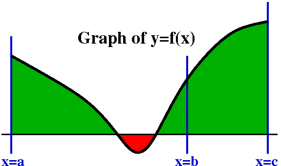 Property (*) and consequences
Suppose a<b<c. Then abf(x)dx+bcf(x)dx=acf(x)dx and I will call this statement
(*). I am happy if you believe this statement. I hope that the picture
to the right is enough verification. The picture has red for area
below the horizontal axis and green for area above the axis because I
wanted to remind you how area is counted for the definite integral. It
is possible to prove this statement from the definition with Riemann
sums.
Unexpected consequences of (*)
While most people are willing to believe (*), there are some results
which may take you some time to learn to use. For example, in the
equation
abf(x)dx+bcf(x)dx=acf(x)dx
what if we change b to a? Then we seem to get
aaf(x)dx+acf(x)dx=acf(x)dx
and the only way this could be true is if
aaf(x)dx=0.
Most people find this easy enough to believe: this quantity is the
area of a "region" with width equal to zero, and some height, and such
an area should be 0. So any definite integral whose upper and lower
limits are the same must be 0.
O.k., if you believe that one, then I will make another change in the
equation:
abf(x)dx+bcf(x)dx=acf(x)dx.
Change c to a in this equation, and use the fact that the
right-hand side will become aaf(x)dx which we already "know" is
0. So we get:
abf(x)dx+baf(x)dx=0
and this certainly means that baf(x)dx=–abf(x)dx
so that when the limits of a definite integral are interchanged, then
the value's sign is changed!
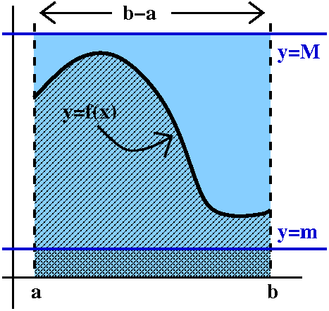 Property (**)
This is extremely useful when you are confused and need to make some
sort of estimate. Suppose, somehow, you know that all of the values of
f(x) on the interval [a,b] are between m and M. That is, you know
m<=f(x)<=M for all of those x's. Then (look at the graph!) the
"area" (actually the definite integral) will be trapped inside a
box. So the result is:
m(b-a)<=abf(x)dx<=M(b-a).
This is because the wiggly region contains the smaller box and is
contained by the larger box. It looks silly, but the estimates can
really be useful in checking computations.
|
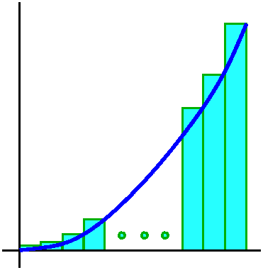
Yet another example ...
Here is a final example of how to compute an area (or a definite
integral) in the most direct fashion: by getting the area of a
collection of approximating rectangles, and then analyzing what
happens as the partition gets "finer".
The example is the area under y=x2 from 0 to 1. This
means the area enclosed by the x-axis, y=1, and y=x2. It is
an area in the first quadrant. We will approximate the area, which is
the definite integral 01x2dx by a collection of
Riemann sums. Here f(x)=x2.
- Partition [0,1] into N equal subintervals, where you
should think that N is some large positive integer. Since the original
interval has length 1, each subinterval will have length 1/N. The
actual partition points will begin 0/N, 1/N, 2/N, 3/N, 4/N ... and
will end with (N-1)/N and N/N.
- Get sample or intermediate points. In this
computation, I will choose the right-hand endpoints of each
subinterval as the sample points. So in the first subinterval
[0/N,1/N], the sample point will be 1/N. In the second subinterval
[1/N,2/N], the sample point will be 2/N. In the third subinterval
[2/N,3/N], the sample point will be 3/N. ... In the Nth
subinterval [(N-1)/N.N/N], the sample point will be N/N.
- Compute the function values at the selected points. These numbers
are the heights of the approximating rectangles, and they are
f(1/N)=12/N2 and
f(2/N)=22/N2 and
f(3/N)=32/N2 and ...
f((N-1)/N)=(N-1)2/N2 and
f(N/N)=N2/N2. Wow!
- Multiply each of the heights by the widths of the rectangles. Each
of the widths is identical, however, so things aren't so bad. The results for the areas of the rectangles are:
12/N2·(1/N) and
22/N2·(1/N) and
32/N2·(1/N) and ...
(N-1)2/N2·(1/N) and
N2/N2·(1/N). More wow!
- Add 'em up. So this is:
12/N2·(1/N)+22/N2·(1/N)+32/N2·(1/N)+...(N-1)2/N2·(1/N)+N2/N2·(1/N).
More compactly written, the Riemann sum is j=1Nj2/N3. I
combined the powers of N "downstairs". You could also pull out the
1/N3 because it multiplies every term in the sum, and then
the result would be (1/N3)j=1Nj2.
N=5
If we had N=5, the approximation would be
(1/53)(1+4+9+16+25) which is (1/125)(55). The mysterious
part is the 55, of course.
A magic formula
Well, everyone knows (it is in the book on page 317, so ... it is possible to know
it!) that j=1Nj2 is
(1/3)N3+(1/2)N2+(1/6)N.
We actually checked that if N=5 is plugged into this formula, the
result is 55. That's nice. So maybe the formula is correct.
Where do these formulas come from? Why are they
correct?
There are lots of amazing formulas like this, and they were discovered
initially to allow people to compute definite integrals exactly
(the definite integrals first occurred as areas or volumes). Next year
I hope to teach a first-year seminar and show people how to discover
such formulas, and, after they are discovered, check that they are
correct. After all, we only checked that the sum of squares formula
was correct for N=5. I have no desire to check directly that it is
correct for N=238, yet I do believe it will give the correct
result. So if you are a first-year student next fall, then ...
Getting the exact value of the definite integral
Since we know that j=1Nj2 is
(1/3)N3+(1/2)N2+(1/6)N and that the Riemann sum
is this divided by N3, then the value of the Riemann
sum is (1/N3)((1/3)N3+(1/2)N2+(1/6)N)
which is (1/3)+(1/2N)+(1/6N2) and certainly as N-->, this must approach 1/3. So 01x2dx=1/3.
Change the problem: make it harder!!!
These techniques seem to be (they are!) very intricate. Let me show
you how to solve this problem by first making it more
difficult. The people who discovered that the (seemingly) more
difficult problem can be solved very neatly really had a lot of
intellectual courage.
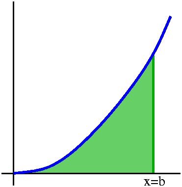 So instead of studying 01x2dx, we will study the
function
So instead of studying 01x2dx, we will study the
function
A(b)=0bx2dx.
We really want to know A(1), but we'll consider this more general
problem anyway.
What do we know?
Well, there is one value of the function that is extremely easy
to compute: A(0)=00x2dx=0.
That seems to be the only simple thing. But this is a CALCULUS course, and maybe we should
try to differentiate A(b). This, which certainly should seem almost
ludicrous, turns out to be the successful approach.
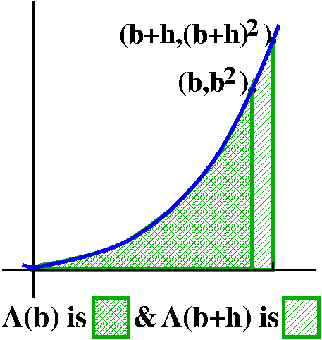 In order to find A´(b) we will need to consider A(b+h)-A(b) and
then divide the result by h.
In order to find A´(b) we will need to consider A(b+h)-A(b) and
then divide the result by h.
Certainly (*) implies that
0bx2dx+bb+hx2dx=0b+hx2dx
so that A(b+h)-A(b) is bb+hx2dx.
But we can use (**) now. f(x)=x2 is increasing on [b,b+h],
so for all x in the interval,
b2<=f(x)<=(b+h)2. So, with m=b2
and M=(b+h)2, we see that
b2·h<=A*b+h)-A(b)<=(b+h)2·h
since h is the width of the interval. Now divide by h:
b2<=[A(b+h)-A(b)]/h<=(b+h)2.
Notice that both estimates -->b2 as h-->0. This means
that A(b) is differentiable, and that A´(b)=b2.
An initial value problem
We have a function, A(b), with the following properties:
A(0)=0 (initial condition);
A´(b)=b2 (differential equation).
This is an initial value problem. All antiderivatives of
b2 have the formula (1/3)b3+C. If
A(b)=(1/3)b3+C then A(0) must be C, but the initial
condition states that A(0)=0, so C=0. Therefore,
A(b)=(1/3)b3.
Now solve the original problem
Since A(b)=(1/3)b3, then A(1)=(1/3). No problem!
Hey, things are easier than they look
In fact it turns out that we didn't need to figure out the C, because
the value we need to compute the integral from 0 to 1 is A(1)-A(0),
and any antiderivative will give the same result (the "+C" adds and
subtracts, and doesn't change the answer).
The Fundamental Theorem of Calculus, version 1
If F´=f, then abf(x)dx=F(b)-F(a).
In fact, the notation usually used "abbreviates" F(b)-F(a) by
F(x)|x=ax=b. And
"Fundamental Theorem of Calculus" is also usually abbreviated as FTC.
Here is how the original area desired would be computed.
- Let's find the area under y=x2 from 0 to 1.
- Recognize that this is the same as computing 01x2dx.
- We know an antiderivative of x2: it is (1/3)x3.
- FTC then declares that the definite integral
(1/3)x3|x=0x=1
and this is (1/3), the value of the area desired.
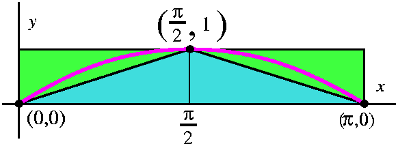 The area under a bump of sine
What is the area undo a bump of sine? Well, first think a bit: the
idea of bump maybe means the area between two places where sine is 0
and where the curve is above the x-axis. So the area would be computed
by the definite integral 0Pisin(x) dx. Usually having some
estimate of the size of a quantity, even before computing, is a good
idea. Otherwise you may make some simple error, and get some result which is a huge mistake.
One overestimate of this definite integral is obtained by
looking at a rectangular box which contains the area. The width of the
box is Pi and its height is 1, so the integral should be less than
Pi·1=Pi. An underestimate of the area could be gotten by
looking at two triangles under the graph. Each has base Pi/2 and
height 1, so the total area of the two triangles is
2·(1/2)·(Pi/2)·1=Pi/2 (the 1/2 comes from the
formula for the area of a triangle). One student suggested 0 as an
underestimate. While that is certainly valid, I like under- and
overestimates which are closer to the exact answer (as long as I don't
have to work very hard!). Now we know
Pi/2<=0Pisin(x) dx<=Pi.
To compute this area exactly, we use FTC. We need an antiderivative of
sine, and that happens to be -cos(x). So:
0Pisin(x) dx=-cos(x)|0Pi=-cos(Pi)-(-cos(0))=-(-1)-(-1)=2. The
(potential!) confusion of minus signs occurs often when applying FTC,
so some care is needed. The exact area is 2, and this is certainly
between Pi/2 and Pi.
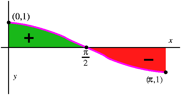 A fake computation: the "area" under a bump of cosine
I then tried to rush ahead and compute the "area" under a bump of
cosine. Or, rather, I compute this definite integral: 0Picos(x) dx. I asserted that the
result should be ... well, should be ... something.
Here is the computation using FTC, since an antiderivative of cosine
is sine.
0Picos(x) dx=sin(x)|0Pi=sin(Pi)-(sin(0))=0-0=0.
What happened to the "area" under the bump? We computed a definite
integral, and that's the limit of Riemann sums, and they count
geometric area under the x-axis negatively. The graph of cosine on the
interval [0,Pi] exactly balances the positive over-the-axis region
with a negative under-the-axis region. So it is 0 both
computationally and geometrically!
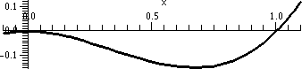 QotD
QotD
I sketched the curve y=x2(x-1) from 0 to 1 as shown to the
right. I asked what the area was inside the bump. I observed that the
function was negative, so the definite integral would be negative, but
the area would be positive.
A solution might go like this:
01x2(x-1)dx=01x3-x2dx=(using FTC)=(1/4)x4=(1/3)x3|01=(1/4)-(1/3)=-1/12.
Therefore the area is 1/12.
| Friday (=Tuesday),
November 21 | (Lecture #23) |
|---|
A question of blood...
 I asked how we could estimate how much blood the heart pumps out to
the body, drawing an especially silly picture on the board (look
left). Knowing the quantity of (hopefully!) oxygenated blood which is
pushed around the body can be a useful part of health assessment. How
can we measure the blood flow through the aorta, the major artery
emerging from the heart? A better diagram of a heart is to the
left. The heart is a very complicated and wonderful pump.
I asked how we could estimate how much blood the heart pumps out to
the body, drawing an especially silly picture on the board (look
left). Knowing the quantity of (hopefully!) oxygenated blood which is
pushed around the body can be a useful part of health assessment. How
can we measure the blood flow through the aorta, the major artery
emerging from the heart? A better diagram of a heart is to the
left. The heart is a very complicated and wonderful pump.
|  |
 The Aztec solution
One method might be to take a knife, preferably an obsidian knife, and
rapidly cut through the chest wall, sever the aorta, and cause the
blood that would flow through it to fill up a bucket. In about five
minutes we'd probably have a good idea of how much blood flows through
the aorta. There are several criticisms possible of this
"protocol". One criticism might be that, well, maybe the person
involved might not be good for much afterwards. Another criticism
could be that this would not show the actual pumping capacity of the
aorta, because maybe within a minute or two some ... difficulties
would occur. In some sense, this Aztec protocol is the ultimate in
what might be called destructive testing. By the way, obsidian
is "a dark glassy volcanic rock formed from hardened lava" and was
actually used for certain similar purposes in that culture.
Another solution: cardiac catheterization
The American Heart Association and the NIH (National Institutes of
Health) both have lots of information about this. Here are some quotes
from these sources:
-
The AHA begins:
"This is a procedure done on the heart. In it, a doctor inserts a thin
plastic tube (catheter) (KATH'eh-ter) into an artery or vein in the
arm or leg. From there it can be advanced into the chambers of the
heart or into the coronary arteries."
- Or from
the NIH:
"Cardiac catheterization is used to study the various functions of the
heart or to obtain diagnostic information about the heart or its
vessels. A small incision is made in an artery or vein in the arm,
neck, or groin. The catheter is threaded through the artery or vein
into the heart. X-ray images called fluoroscopy are used to guide the
insertion."
Very much simplified ...
Imagine a thin plastic coated wire inserted into your circulatory
system and threaded up into the aorta. At the end of the wire is a
sort of microscopic windmill: a bunch of little fans which spin as the
blood flows. As they spin, they move a bunch of wire around a
magnet. Since magnetism+movement+wires=current ( a wonderful
fact!), electric current is created and passed back through the wire
into a measuring device. This is certainly very much simplified. Now I
will further simplify and imagine some numbers. This is not reality,
but a math course! The following numbers are invented, and the whole
purpose of this "exercise" is to get you to think about what's going
on.
| Elapsed time | Fluid flow rate |
|---|
| 1 min | 30 cm3/min |
| 2 min | 20 cm3/min |
| 4 min | 40 cm3/min |
| 5 min | 25 cm3/min |
The blood flow will be given in cm3/min (cubic centimeters
per minute) and the time will be measured in minutes since the
beginning of the procedure. The information learned is displayed to
the right.
This isn't much information. But how can we use what we've learned? A
standard way to use these numbers is the following. It is certainly
very approximate in this case.
At the end of the first minute, we're told that the flow is 30
cm3/min. Hey, we could estimate how much blood is
pumped by making the assumption that the flow rate is constant during
the time interval involved. Then we see that
30 cm3/min·1 min=30 cm3
(flow rate multiplied by duration) would be pumped. I am not
asserting that this is necessarily correct. It is an estimation. We
are using the information, and the method is very simple. Similarly,
during the second minute, we can estimate that
20 cm3/min·1 min=20 cm3 is
pumped. The flow rate changed during the second minute. We're faced
with a slightly different "challenge" in using the third line of the
table. It has elapsed time (since the start of the procedure) as 4
minutes. So the duration has now changed from 1 minute to 2
minutes. (Why? Well, y'know, in the real world things maybe don't work
as you'd like. Maybe the machine broke, or the technician didn't pay
attention, or ... in any case, we need to work with the data we have!)
So during those two minutes, we have (flow rate·duration)
an estimate of
40 cm3/min·2 min=80 cm3
blood pumped. Finally, in the last minute of this procedure, we
estimate that
25 cm3/min·1 min=25 cm3.
Let me abbreviate just a bit. The units are repetitive and I will omit
them (this is a math course!). So here are the essential details of
the computation:
30·1+20·1+40·2+25·1=155.
That's what we're computing.
If we wanted a picture of the computation, maybe what is shown to the
right gives you some idea. The dots represent the actual known
data. The area of the rectangles shown is given by the product of the
appropriate flow rate and duration. Yes, there are other possible
approximations using the data given. We will study some of them in
Math 152, but here only a rather simple-minded approach will be used.
|
 |
More information
| Elapsed time | Fluid flow rate |
|---|
| 30 sec | 32
cm3/min |
| 1 min | 30
cm3/min |
| 1 min 30 sec | 28 cm3/min |
| 2 min | 20
cm3/min |
| 2 min 30 sec | –6 cm3/min |
| 3 min | –8 cm3/min |
| 3 min 30 sec | 34
cm3/min |
| 4 min | 40
cm3/min |
| 4 min 30 sec | 43
cm3/min |
| 5 min | 25 cm3/min |
Now let's refine the data. Let me suppose that we have no "technical"
problems, and that we are recording the flow rate every 30 seconds.
We could imagine the numbers given in the table to the right. Please
notice that the data we've already obtained is part of this table -- I
am imagining that we're measuring the same process as before, only we
are sampling things more often. Here we have readings every thirty
seconds with no data points are omitted. So we actually have 10 pairs
of numbers.
There is another complication which has occurred, and I hope you
notice it. Some of the flow rates (2 min 30 sec and 3 min)are
negative. Could this happen? Well, actually maybe yes. The
heart is a terrific pump but maybe sometimes things don't always
synchronize well or work perfectly: maybe the heart valves don't close
all the way or don't close at precisely the correct time in the
pumping cycle, etc. This complicates our task. We could ask what the
heck we want to measure in this situation, and several answers are
possible. We might want to measure the total pumping effort of the
heart. Or we might want to know the net amount of oxygenated blood
which is pushed out into the body. Let me look at the second
quantity. In that case, the negative flow rates affect the total blood
pumped because, indeed, that amount in that time should be
subtracted, just like the sign of the flow rate indicates, from
the total.
|
What should be computed here? If we do flow rate multiplied by
duration, we should be consistent (the units!) and realize that, for
example, 3 min 30 sec is 3.5 minutes. So the numerical computation
here is
32·.5+30·.5+28·.5+20·.5+(-6)·.5+(-8)·.5+34·.5+34·.5+40·.5+43·.5+25·.5=119.
And this estimate, using this data, is 119 cm3. This is
much less than the earlier figure, I guess because the data at 4
minutes over a duration of 2 minutes led to a big overestimate.
 A picture of what we computed is to the right, which I sort of laid
over the old bar chart whose outlines where visible are indicated with
dashed lines. I put in the new data points, and then the computation
above is indicated by the areas of these rectangles. But the
total area of the rectangles which are below the horizontal axis is
subtracted from the total. Can you "see" the change from 155 to 119?
A picture of what we computed is to the right, which I sort of laid
over the old bar chart whose outlines where visible are indicated with
dashed lines. I put in the new data points, and then the computation
above is indicated by the areas of these rectangles. But the
total area of the rectangles which are below the horizontal axis is
subtracted from the total. Can you "see" the change from 155 to 119?
|
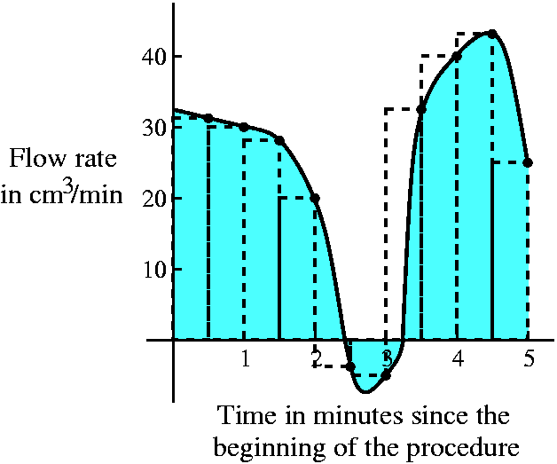
Ideally ...
You might imagine that ideally we make lots and lots of measurements
(in fact, this is more like what is done, because I think there is a
computer recording the flow rates very frequently and then making the
computations that I'm discussing in such a silly way). What should we
think about? We could have lots and lots and lots of data points. And
then the rectangles get very thin. And then the data points look very
much like a curve. The number that's wanted is the total blood pumped
out to the body, but the picture which might result could look a lot
like what is shown here. I have again overlaid it with the rectangles
from the previous discussion. So it seems there might be some kind of
flow rate curve, and that the blood pumped out to the body, the net
blood out, is the area of the colored regions above the curve
minus the area of the colored region below the curve.
I hope that you can see some resemblance between this and the
discussion of the area of the hand which we did previously. Here we
are approximating quantities of liquid, and there we were trying to
approximate areas. It turns out that this computational idea can be
applied in many situations, and it is used in essentially all fields
of engineering and applied science. I now need to tell you the
official vocabulary.
|
Vocabulary
Start with the following: a function f defined on an interval [a,b].
- Partition A partition of [a,b] is a collection of
points in the interval always starting with a and ending with b. It
looks like this:
a=x0<x1<x2<...xn-1<xn=b
- Subintervals Each partition defined a collection of subintervals. Here they are:
[x0,x1] and [x1,x2] and
[x2,x3] and ... [xn-1,xn].
If there are n+1 points in the partition (counting from 0 to n) then
there are n subintervals. The length of each subinterval is important,
and the length of the first subinterval is
x1-x0. This is frequently abbreviated x1. So the length of the
jth subinterval, xj-xj-1, would be
abbreviated xj. The
Greek letter , Delta, is used
as an abbreviation of Difference.
- Sample points or intermediate points You select an
intermediate point in each subinterval. The text uses the phrase
"intermediate point". The phrase "sample point" is what I am used to,
and I think it is more widely used. It also makes me think more of
physical measurements. I will try to use both phrases. The text uses
the letter cj for the jth sample point. So
cj would be inside [xj-1,xj], and
therefore xj-17lt;=cj<=xj.
- Computing the sum The textbook uses the notation R(f,P,C)
to mean Riemann sum depending on the function, f, the partition, P,
and the choice of sample points, C. I don't know any generally
accepted notation so let me stick with what is in the book. Anyway,
here is the formula for the Riemann sum:
f(c1)x1+f(c2)x2+...+f(cn)xn.
This is too long to write and usually if people have to work with such things, they will write
j=1nf(cj)xj
What this means geometrically ...
To the right is my attempt to show you what a Riemann sum might look
like. But I've made it quite simple. There are only seven
subintervals, and the curve which is the graph of f(x) is also not too
complicated. The dots on the x-axis denote the sample or intermediate
points, and the vertical lines above them are the lengths
f(cj). The boxes have areas which are equal to the pieces of
the Riemann sum, f(cj)xj.
The f(cj) is the height and the xj is the width of a rectangle.
| 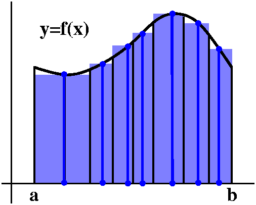
|
An example
To the left is a graph of a function, y=f(x), where f is defined on
the interval [0,5]. f's graph is two line segments, the first
horizontal from (0,1) to (2,1) and the second tilted from (2,1) to (3,0),
followed by the lower half of a circle of radius 1 centered at
(4,0), a circular arc going from (3,0) to (4,-1) to (5,0).
|
|
|
Here are some partitions, choices of sample points, and the resulting
Riemann sums.
|
Partition 0, 2, 3, 5.
Sample points 1, 3, 4.
The function values at the sample points are:
f(1)=1, f(3)=0, f(4)=-1.
Riemann sum 1(2-0)+0(3-2)+(-1)(5-3)=0.
|  |
Choosing the sample point at 3 gives a zero contribution to the Riemann sum.
|
Partition 0, 2, 3.5, 5.
Sample points 1, 3, 4.
The function values at the sample points are:
f(1)=1, f(3)=.5, f(4)=-1.
Riemann sum 1(2-0)+.5(3.5-2)+(-1)(5-3.5)=1.25.
| 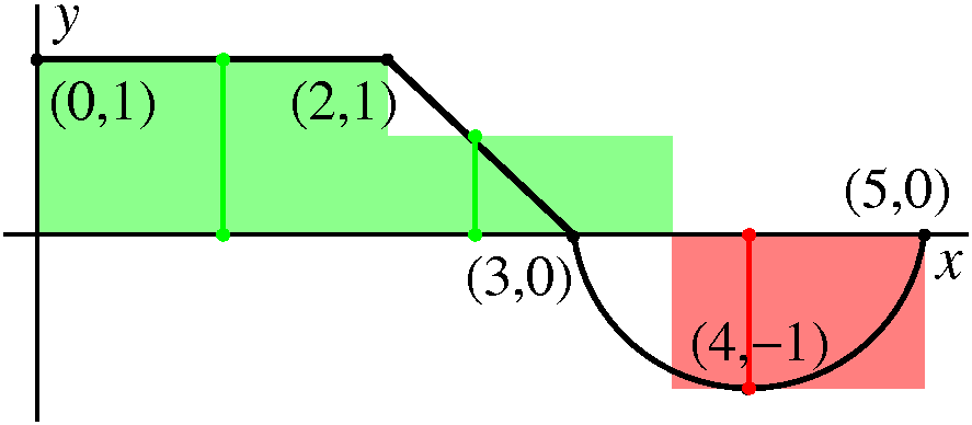 |
Partition 0, 2, 3.5, 4.5, 5.
Sample points 2, 2, 4, 5.
The function values at the sample points are:
f(2)=1, f(2)=1, f(4)=-1, f(5)=0.
Riemann sum 1(2-0)+1(3.5-2)+(-1)(4.5-3.5)+0(5-4.5)=2.5.
| 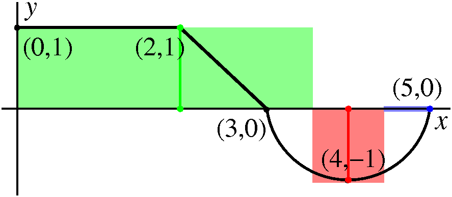 |
The definition allows the sample point to be on the boundary of the
subinterval, so two adjoining subintervals could possibly share their
sample points. This is a bit wasteful in terms of information,
though.
Also notice that the rectangle on the rightmost interval
has height 0.
|
Partition 0, 1, 2, 3, 4, 5.
Sample points .7, 1.44, 2.5, 3.5, 4.75.
The function values at the sample points are:
f(.7)=1, f(1.44)=1,
f(2.5)=.5, f(3.5)=-sqrt(3/4)-.866, f(4.75)=-sqrt(7/16)-.661.
(The numbers for f's values at 3.5 and 4.75 come from the equation of
the lower unit semicircle, -sqrt(1-x2), suitably translated
to the right.)
Riemann sum 1(1-0)+1(2-1)+.5(3-2)+(-.866)(4-3)+(-.661)(5-4)=.973.
| 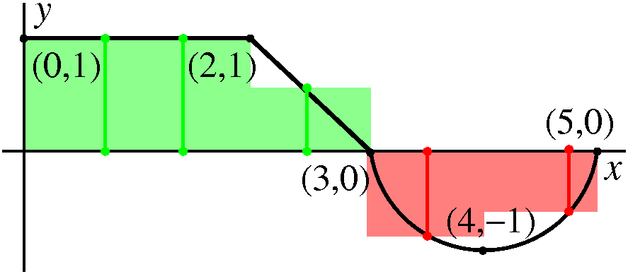 |
|
Notice that putting another sample inside the interval from 0 to 2
didn't improve the approximation very much. If taking samples is
difficult or expensive (and it might be in real life!) then probably
increasing the sampling where functions wiggle a lot rather than where
the values are (relatively) constant is a good idea. This is, in fact,
what the approximation strategies inside most calculators try to do.
Part of the impression I would like to leave with you, even with just
a few examples, is that Riemann sums can be quite complicated
objects. They can be irritating to compute, and there are so many of
them that understanding them may be difficult.
|
If the partition gets finer and finer ...
Suppose that the largest length of the subintervals defining the
Riemann sums gets shorter and shorter. Then if you look at the
picture, you might hope that all the Riemann sums, no matter how you
select the intermediate points (just so they stay inside their correct
subintervals, though) will approach one specific number. In the case
of the function whose graph is shown above, my candidate for specific
number would be the area of a 2-by-1 one rectangle (2) added on to the
area of a 1-by-1 right triangle (1/2) and then minus the area of half
a circle of radius 1 (-Pi/2). So for that specific function, the
Riemann sums will get close to 2.5-Pi/2.
The definite integral
Suppose some more general function f is defined on an interval [a,b},
and suppose either that f is continuous or piecewise continuous (that
is, continuous except for a few jumps). Then as the maximum length of
the subintervals used in the Riemann sums for this function get
smaller, the values of the Riemann sums will approach a unique number
which is called the definite integral of f on the interval
[a,b], and the notation used is
abf(x)dx.
Here a is called the lower limit and b is called the upper limit. The
integral sign, , is a sort of
stylized abbreviation of the word Sum. The function f(x) is
sometimes called the integrand. The "dx" is there to remind you of the
length of little subintervals.
Exams
The exams were returned. Here is one version, with some answers. The grading is discussed here.
| Friday,
November 16 | (Lecture #22) |
|---|
An exam was given, with answers now available, along with a discussion of the grading.
| Tuesday,
November 13 | (Lecture #21) |
|---|
We are about to jump into something that will seem very different. But
there will be a remarkable connection between this topic and what we
have already studied which will be revealed in a few lectures. I will
begin with a seemingly silly question.
 Hand area
What is the area of my hand? There was, of course, some laughter. But
the question and other similar inquiries, while superficially silly,
is actually quite important. Appropriate drug doses are sometimes
calculated in terms of BSA, body surface area. This is
especially important when prescribing drugs for infants or drugs with
strong side-effects (for example, some drugs used in cancer
treatment). And knowledge of body surface area is important in trying
to understand heat balance when people exercise. There are many
formulas for BSA.
So my question is much more modest: how can we compute the area of my
hand? We discussed this. There are many methods, but if you think
about area, there are really not very many shapes whose area we can
compute exactly. The most important and simplest shape is a rectangle,
where we know the area is the product of the length and width. We
should try to take advantage of this. So look at an image of my hand,
and ... well, after discussion we came up with this (mostly at the
suggestion of Mr. Chang):
- Superimpose a square grid over an image of my hand.
- Put boxes inside.
- Put boxes outside.
- Count the boxes totally inside. Count the boxes which contain any
(even little!) piece of the hand image (these are the "outside"
boxes).
- Compute the area of the inside boxes and the area of the "outside"
boxes.
- The hand area will be between the inside box area and the outside box area.
Let me "implement" (!) this and get some information.
|
I'll suppose first that I put the image of the hand in a square grid
which is, say, 1 mm (millimeter) on a side. I don't know if this is
physically too reasonable, but, what the heck, I could get something
that looks like the picture to the right.
Then I could count the grid boxes which are entirely within
the hand image. There was some objection to this, because, you see, I
could always be a little clever (?) and maybe sort of count some boxes
which are almost entirely in and then compensate by dropping the count
by 1 if I count a bunch of those.
|
 |
|
I commented that I wanted a process (an algorithm) which could be done
totally "mechanically", leaving nothing to choice, and which was
extremely simple-minded.
|
|
I'll suppose first that I put the image of the hand in a square grid
which is, say, 1 mm (millimeter) on a side. I don't know if this is
physically too reasonable, but, what the heck, I could get something
that looks like the picture to the right.
I think if I count correctly there are a total of 18 boxes entirely inside the hand image.
| 
|
|
Now for an overestimate. Let me start with the boxes which are
entirely inside, and then add on any boxes that have even the
slightest "tinge" (?) or hint of the hand image inside. Again, maybe
there are objections: we could be cleverer (?) and sort of estimate
how much of a box is inside, etc. But then we would have to make
decisions, and some of those decisions maybe could be difficult. Here,
if we have a simple-minded scheme, I'll bet that any two people will
come up with the same answer. At least we get a result that's stable,
and probably doesn't depend on the observer too much.
There are 18 all-inside boxes, and (if I count correctly!) 60 more
boxes are needed to cover all parts of the hand image. The total of
the outside boxes is therefore 78.
|
|
The result?
If I believe that area of bigger shapes is bigger, then I see that the
area of the hand is between 18 mm2 and 78
mm2. And there is a huge gap between these over- and
underestimates of 60 mm2.
More information?
How can we improve this? That is, how can we get over- and
underestimates which are closer to the actual area of the hand, so
the gap will be smaller? We discussed this. The idea of improving the
estimates is not totally obvious, and the whole procedure that's being
discussed in this lecture evolved over many centuries in at least 4
different cultures (in China, Greece, India, and perhaps also in Egypt
and associated cultures). Lots of smart people thought about it.
|
|
We get try a grid with more subdivisions: this is called
refining the grid. Again, I believe that Mr. Chang thought that we should just halve
the size of the square sides. Maybe the result is something like what
is shown to the right.
Now the idea is maybe not so easy to implement, at least for human
beings whose eyesight and counting ability is not so perfect. But we
can try anyway.
|

|
|
Well, if I have counted correctly, there are 63 new squares which are
completely inside the hand image. This is in addition to the 18
old squares. But, wait: the new squares have sides which are half the
length of the old squares. So each of the new squares has one quarter
the area of the old squares. So actually we have now succeeding in
underestimating the area by 18+(63/4)=25 and
7/8.
|  |
|
Now let's get an overestimate. We need to add on all of the little
squares which contain any part of the hand image. If I have counted
correctly (!!) there are 118 of them. That means we need to add one
quarter multiplied to 118 to the previous underestimate in order to
get the corresponding overestimate. So 118/4 is 29 and a half. Add
this on to the previous 25 and 7/8, and the overestimate is
45 and 3/8.
|
|
Underestimate, overestimate, and gap
Let me summarize what we have done:
| | Underestimate | Overestimate | Gap |
|---|
| 1-by-1 squares | 18 | 78 | 60 |
|---|
| 1/4-by-1/4 squares | 25.875 | 45.375 | 29.5 |
|---|
| And so on ... |
|---|
The secret is that this sort of approach is just about all we
can do with real physical quantities. You can really only make better
(or worse!) estimates: over- or underestimates. The ideas outlined
here, taking finer and finer grids, will lead to overestimates which
shrink and underestimates which increase, so that (we hope!) the gap
between them -->0: refine until you get as close as you want. And
this is about all we can do. I don't think the situation is hopeless,
but I do think it is compicated.
Attribution
The neat idea of asking for the area of "my hand" is something I
borrowed from Professor J. Rosenstein
of our math department. I think it is neat. It is a question which
brings up important ideas immediately and clearly.
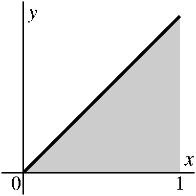 An exact computation
Mr. Spero asked if we could do an exact
computation, and this I was happy to try, since many people seemed
rather distressed about the statements made previously. So I will
present a simple example of a general idea. The general idea is very
successful, although the simple example may seem to be
overelaborate. I will try to compute the exact area "under" y=x for
the interval [0,1]. (Yes, I am aware that we know this area --
the ideas are what is important -- as soon as we get the ideas we'll
be able to do much more complicated computations.)
How to begin
We will try to get over- and underestimates of the area We could
divide the interval [0,1] into 4 equal parts using 0 and 1/4 and 2/4
and 3/4 and 1, which I'll choose to call 4/4.
Then put rectangles underneath y=x in each
subinterval. We will be slightly economical and put the largest
rectangles we can under the y=x, but we will be slightly simple-minded
and only look at rectangles which have sides parallel to the
coordinate axes. Then we compute the area of these rectangles: 0 1 1 1 2 1 3 1
--- · --- + --- · --- + --- · --- + --- · ---
4 4 4 4 4 4 4 4
The 1/4's come from the width of the rectangles, and the varying
heights (even including the somewhat absurd 0/4) from the heights of
the rectangles.
| 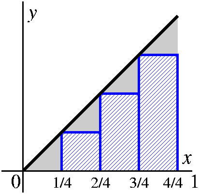
|
Now we need an overestimate, and the true area will
be "captured" between these two estimates. Again, we will use the
interval divided into 4 equal pieces, and rectangles with sides
parallel to the coordinate axes which just contain the region of
interest to us. So the area of these rectanges is: 1 1 2 1 3 1 4 1
--- · --- + --- · --- + --- · --- + --- · ---
4 4 4 4 4 4 4 4
| 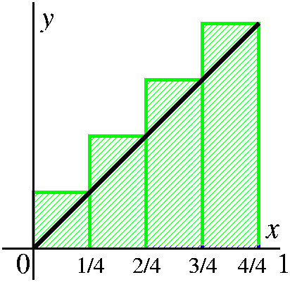 |
|
Finally, if we want to see how much gap or error
there is between these over- and underestimates, we can look at the
area that is inside the big rectangles and outside the small
rectangles. The result (because y=x is so simple!) is 4 squares, each
with side length 1/4. So the gap is 4(1/4)(1/4)=1/4.
| 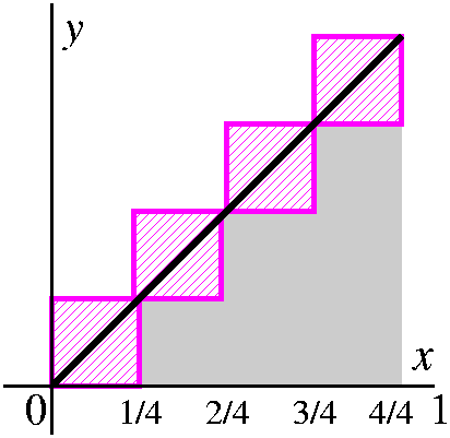 |
The whole setup
We could do something similar with other numbers of
subdivisions of [0,1]. Here are some numerical results:
# of
subdivisions | Underestimate | Overestimate | Gap |
|---|
| 4 | .37500 |
.62500 | .25000 |
|---|
| 10 | .45000 |
.55000 | .10000 |
|---|
| 25 | .48000 |
.52000 | .04000 |
|---|
| 100 | .49500 |
.50500 | .01000 |
|---|
What really happens, in general
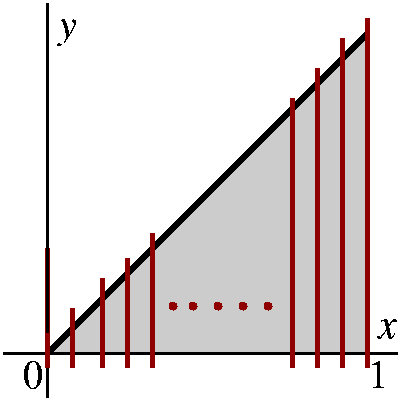 Here it helps to get a little bit abstract. Suppose we divide the
interval [0,1] into n equal pieces, where you should think that n is
some large integer. Then the underestimate will have total area (using
heights over the left-hand endpoint of each subinterval shown in the
diagram to the right)
Here it helps to get a little bit abstract. Suppose we divide the
interval [0,1] into n equal pieces, where you should think that n is
some large integer. Then the underestimate will have total area (using
heights over the left-hand endpoint of each subinterval shown in the
diagram to the right)
  0     1      1     1      2     1      3     1          n-1    1
 --- · --- +  --- · --- +  --- · --- +  --- · --- + ··· + --- · ---
  n     n      n     n      n     n      n     n           n     n
In fact, we can "massage" this underestimate a bit and get for the underestimate:
(1+2+3+...+(n-1))·(1/n2).
The overestimate uses the heights over the right-hand endpoint of each
subinterval, and then the overestimate is:
(1+2+3+...+n)·(1/n2).
The gap between the over- and underestimates is
n·(1/n2)=1/n.
So what happens as n-->? Since the gap is 1/n, this will
-->0. So let me look at the overestimate. This is
(1+2+3+...+n)·(1/n2). Let's get a formula for
1+2+3+...+n.
A formula
You may remember the trick (maybe done in high school when you studied
arithmetic progressions). The trick is writing two versions of the sum
in oppositite order. Look:
 1 +   2   +   3   +   4   + ... + (n-1) + n
 n + (n-1) + (n-2) + (n-3) + ... +   2   + 1
Now add the sums columnwise. So we get 1+n which is n+1 and 2+(n-1)
which is n+1 and ... all of the column sums are the same (that's right
because the top is going up by 1 each step while the bottom is going
down by 1 each step). There are n of the n+1's, so the total of all of
the numbers is n(n+1). But this is two copies of the sum we want, so
we need to divide by 2.
I think we have verified that 1+2+3+...+(n-1)+n is [n(n+1]/2. And the
overestimate of the area, is this divided by n2. So a
formula for the overestimate is [n(n+1]/[2n2]. What happens
to this as n-->? Well, we have studied such limits, and we could
either divide top and bottom by n2 or we could use L'H
twice. In any case, the limit will be 1/2.
A spectacular result?
I have now proved (done an exact computation!) that the area of
the triangle is 1/2. And I guess I knew that. But this whole approach
is a template for more complicated reasoning.
Notation
We will need some notation. Lots of sums occur when we do area
computations, and also many other computations. So a special way of
writing these sums which takes less space has been developed. The
Greek capital letter sigma, , is used. Here are some examples:
| Examples of summation notation |
|---|
| Written out | Abbreviated |
| 1+2+3+4+5 | j=15j |
| 32+42+52+62 | j=36j2 |
| {1/2}+{1/4}+{1/6}+{1/8} | j=14{1/[2j]} |
| 1-2+3-4+5 | j=15(-1)j+1j |
The notation, once you get used to it, is wonderfully economical. I should remark that the summation index, which is j in all of the examples above, doesn't really matter. That is
j=13j4 and
k=13k4 both mean the same thing,
which is 14+24+34.
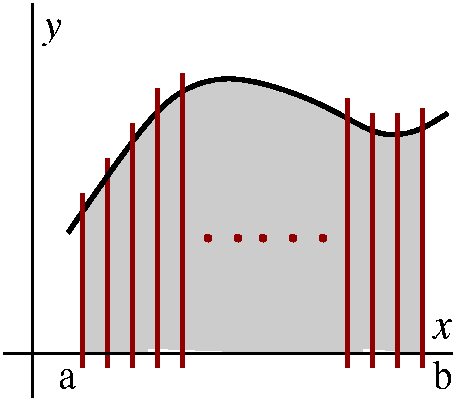 How to approximate area
Suppose that we have a function, f, defined on an interval [a,b] and
we want to compute the area under y=f(x). That's the area bounded by
the x-axis (y=0) and the lines x=a and x=b on each side, and by the
curve y=f(x) on top.
We can get approximations to the area of by dividing the interval into
n equal parts (people don't always use equal parts, but we're just
starting out!). Then we can look at "sample points" in each
subinterval, compute f's value at those sample points, and multiply
those heights by the widths of the subinterval to get areas of
rectangles. Then (sigh!) finally take the sum of these rectangles, and
that will be an approximation to the area we want to compute.
The textbook explains in detail how to write the approximating
sums. In particular, it identifies three sums corresponding to three
choices of sample points: left and right endpoints of subintervals,
and the midpoints of subintervals. Below are the formulas, which you
should not memorize, and what are supposed to be pictures of a
piece of the graph of y=f(x) over (relatively) tall and (relatively)
narrow subintervals with the areas of the relevant boxes displayed.
Since the interval has length b-a, the width of each subinterval is
{b-a}/n. Do not memorize but do try to understand.
Left-hand
endpoints of subintervals |
(j=1nf(a+[{j-1}/n]))({b-a}/n) | 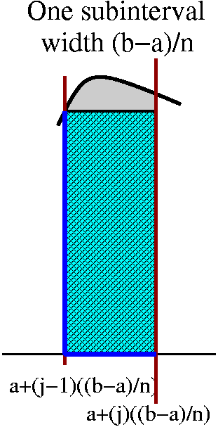 |
Right-hand
endpoints of
subintervals |
(j=1nf(a+[{j}/n]))({b-a}/n) | 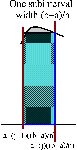 |
Midpoints of
subintervals |
(j=1nf(a+[{j-1}/n]))({b-a}/n) | 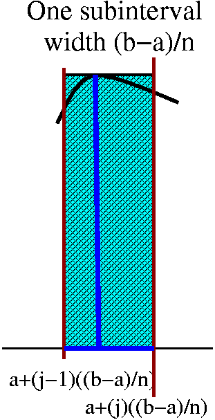 |
QotD
I don't remember! I think it was something like "Compute j=13(j2+{1/j})". This is
(95/6).
Maintained by
greenfie@math.rutgers.edu and last modified 11/13/2007.