| Date | What happened | ||||||||||||||||||||||||||||||||
|---|---|---|---|---|---|---|---|---|---|---|---|---|---|---|---|---|---|---|---|---|---|---|---|---|---|---|---|---|---|---|---|---|---|
| 5/5/2003 |
Let's analyze and prove one version of the Fundamental Theorem of Calculus (FTC). This is discussed in section 7.3 of the text.
In what follows, we will need to "recall" some facts about the Riemann integral.
Proof: If x<y, then F(y)=intayf= intaxf+intxyf by additivity on intervals (4/28 lecture). Since F(x)=intaxf we see that F(y)-F(x)=intxyf. If we know that -M<=f(x)<=M, then -M(y-x)<=F(y)-F(x)<=M(y-x) so that |F(x)-f(y)|<=M|x-y|. Comment: the function g(x) which is 0 if x<0 and is sqrt(x) if x>=0 does not satisfy a Lipschitz condition in any interval which includes the "right side" of 0 because sqrt(x) doesn't satisfy the Lipschitz property in such an interval (see the lecture on 4/14, please). So this g can't be a F corresponding to any Riemann integrable f. The same is true for other functions which don't satisfy Lipschitz conditions. Generally, people expect that "integrating" makes functions "smoother" and better behaved. Thus, we go from Riemann integrable to Lipschitz. Along this line is the next result, which says we go from continuity to differentiability.
Theorem (a version of FTC) Suppose f is Riemann integrable on
[a,b]. Then f is Riemann integrable on [a,c] for all c in [a,b], and
if F(x)=intaxf for x in [a,b], and is f is
continuous at c, F is differentiable at c and F'(c)=f(c). Although this result is almost always used where f is continuous in the whole interval, so F is differentiable in the whole interval with F'=f, we actually don't "need" continuity of f. Here's a fairly simple example of discontinuities in f not "noticed" by F. Suppose f(x) is 1 if x=1/n for n in N and f(x)=0 otherwise. Then f is Riemann integrable in any interval (!) and intabf is 0 for any a and b. Therefore a candidate F will always be 0 and will be differentiable everywhere, and F'=f for x not equal to 1/n. F doesn't notice F's values on a thin set like {1/n}. Of course if we make f non-zero on a "thicker" set then we may run into trouble. We have already seen examples where f is not Riemann integrable as a result (f(x)=1 if x is rational, or even f(x)=x if x is rational). If we had also verified the Mean Value Theorem, then we would know that two differentiable functions defined on the same interval with the same derivative would differ by a constant. That would be enough when combined with our version of FTC to prove that if G'=f on [a,b] and f is Riemann integrable, then intabf=G(b)-G(a). This is the version of FTC which is used everywhere in calculus and associated subjects. Please look at the review material for the final. | ||||||||||||||||||||||||||||||||
| 5/1/2003 |
The final is scheduled for
Tuesday, May 13, 12:00-3:00 PM in SEC 205Professor Cohen has created even more notes on Riemann sums, a total of 21 pages now. Please take a look. Material related to what I discuss today is covered in the textbook in section 5.6 (see 5.6.1 through 5.6.4) and in section 7.2 (see 7.2.7). In probability one builds models of "chance". The cdf (cumulative distribution function) of a random variable X, which is defined by f(x)=probability{X<=x} contains most of the useful probability information. Quantities such as the mean (expectation) and the variance can be computed from it (usually involving various integrals). The function I'd like to study today has the essential properties of a cdf which are listed below. I won't discuss a probability "model" that this function might come from.
Theorem Suppose for all x, y in R, if x<y, then f(x)<=f(y). Then the limit of f(x) as x-->a- exists and is equal to sup{f(x):x<a}. Proof: Let's call the set {f(x) : x< a}, W, and call its sup, S. Why should S exist? We will use the completeness axiom. W is not empty (since, for example, f(a-33) is in W). W is bounded above, and one upper bound is f(a) (this uses the increasing assumption, of course). Therefore S exists using the completeness axiom on the set W, which is non-empty and bounded above. I claim that the stated limit exists. This is a one-sided limit, so the following implication must be verified: if epsilon>0 is given, then there is a delta>0 so that if a-delta<x<a, then S-epsilon<f(x)<=S. Since S is sup{f(x) : x< a}, given epsilon>0, there will be w in W so that S-epsilon<w<=S. But w is a value of f, so that there is v<a with f(v)=w. Take delta to be a-v. Then if a-delta<x<a, we know that a-(a-v)<x<a, so v<x<a. Since f is increasing, we may "apply" f to this inequality and get f(v)<=f(x)<=f(a). This means that w<=f(x)<=f(a). But w>S-epsilon, and since x<a, f(x)<=S because S is the sup of W. Now we have S-epsilon<f(x)<=S, which is what we wanted and the proof is done. Of course a similar statement is true about limits "on the right" with sup replaced by inf. Now I'll begin creating a weird example. We know that Q is a countably infinite set (go back and look at the first day or two in this course). In fact, Q intersect any interval of positive length is countably infinite. Countably infinite means that there is a bijection (a pairing, a function which is 1-to-1 and onto) between N, the positive integers, and the set. So there is a bijection B:N-->{elements of Q, the rational numbers, in the open interval (0,1)}. Now remember that the sumn=1infinity1/2n is 1. So what's f(x), finally? f(x)=the sum of 1/2n for those n's which have B(n)<=x. This is a weird definition. Since the range of B, the bijection, is only the rationals in (0,1), if x is less than or equal to 0, there are no B(n)'s less than or equal to x. Therefore the sum is "empty", and the legal (?!) interpretation of an empty sum is 0. Thus f(x)=0 for x<=0. Now if x>=1, all of the rationals in the open interval (0,1) are below x, so f(x) must be 1. Notice also that f's values are some sort of "subsum" of the complete sum of 1/2n for n in N, and therefore f(x) must be in [0,1] for all x. So we have verified requirements 1 and 2 and 3 for cdf's above. Things will get even more interesting when we look at #4. If x<y and x and y are in the unit interval, then the interval (x,y) has infinitely many rational numbers between 0 and 1 in it. Therefore f(x) must be strictly less than f(y). Thus, on [0,1], f is a strictly increasing function: f(x)<f(y) if x<y. This is more than #4 requires. We saw that #4 implies that the left and right hand limits exist. So all we need to do is investigate where f is continuous. Well, since limx-->a-f=sup{f(x):x<a}=LEFT and limx-->a+f=inf{f(x):x>a}=RIGHT we just need to think about where f(a) fits. Certainly since f is increasing, we know that LEFT<=RIGHT. We'll say that f has a jump at a if LEFT<RIGHT, and the amount of the jump is RIGHT-LEFT. Can f have a jump of, say, 33? That is, can RIGHT-LEFT be 33? Since f's values are in [0,1], I don't think this is possible. Can f have a jump of 1/33? It could have such a jump, but it actually couldn't have too many of such jumps: it certainly couldn't have more than 33 of those, because notice that f can't jump down, only up, since f is increasing. Actually the total length of the jumps of f should be 1, since f(large negative) is 0 and f(large positive) is 1. Now where do the jumps take place? Let's imagine an example, where, say B(17)=3/7. If x<3/7, the sum for f(x) would not have the 1/217 term in it. As x increases "towards" 3/7, f(x) would increase towards sumB(n)<3/71/2n, which would be sup{f(x):x<3/7}. If x>=3/7, the sum would have the term 1/217. And inf{f(x):x>3/7} would be exactly 1/217 larger than sup{f(x):x<3/7}, and would be equal to f(3/7). In fact, f has a jump of 1/2n at B(n): f has jumps at every rational number. The total sum of the jumps at the rationals is 1/2+1/4+1/8+...=1. There are no other possible jumps, since any additional jump would mean that the function increases more than 1, and we already know this is not possible.
In [0,1], this f is continuous at every irrational number and is
continuous at 0 and at 1, and is not continuous at every
rational number between 0 and 1. Is f a cdf of a continuous
distribution? Is it a cdf of a discrete distribution? Well, maybe f
shares aspects of both kinds of distributions.
Is f Riemann integrable on [0,1]? Of course this is the same as asking if, given epsilon>0, we can find a partition P of [0,1] so that US(f,P)-LS(f,P)<epsilon. For example, suppose we take epsilon=1/10. Is there some partition which clearly satisfies the requirement? Remember that f is increasing on [0,1], and f(0)=0 and f(1)=1. If we partition [0,1] into n equal subintervals of width 1/n, then the difference US(f,P)-LS(f,P) must actually equal the total increase (1) multiplied by the width of the subintervals (1/n), so the difference is 1/n. And if n>10, we have a satisfactory partition. And by the Archimedean property, we can always find n so 1/n<epsilon. In fact, any increasing function must be Riemann integrable. Any decreasing function must be Riemann integrable. There are problems with integrability when there is much combined "wiggling" up and down. What is the Riemann integral of f on [0,1]? Some thought should convince you that we know approximately what the integral is: it must be between 0 and 1. But I don't know more than that. In fact, until after this lecture I really didn't think much about what f looks like. So here is what I did: I asked Maple to "draw" an approximation of the graph of an f. I listed 30 rational numbers between 0 and 1, and had Maple draw the approximation to the graph of f by just using these thirty rational numbers, in order, as B(1), B(2), ..., and B(30). The total "weight" that's left over sums up to at most 1/230 which is less than 10-8, a very small number. So the graph drawn is quite close (probably beyond screen resolution) to a "true" graph of f. Here are the Maple procedures I used. gen:=rand(1..99999);This asks Maple to create a "random" integer between 0 and 99,999. A:=[seq((gen()/100000),j=1..30)];n:=30;This asks Maple to create a sequence of "random" rationals (the integers divided by 100,000) in the open unit interval. It assigns this sequence to the name A. The next statement creates the variable n with value 30. bin := proc(x)
local y, inc, j;
global A, n;
y := 0;
inc := .5;
for j to n do
if A[j] < x then y := y + inc fi; inc := .5*inc
od;
RETURN(y)
end;
The procedure bin uses the global variables A and n to get
values of the function f(x) depending on the specifications of A and
n.
area := proc()
local y, j, inc;
global A, n;
    y := 0;
    inc := .5;
    for j to n do y := y + (1. - A[j])*inc; inc := .5*inc od;
    RETURN(y)
end;
This Maple procedure gets the area of the approximation to the
function.
I then plotted the approximation with the command
plot(bin,0..1,thickness=3,color=black); 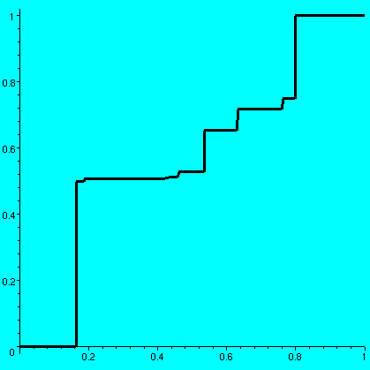 One value of A is this:
   8193   79919   3341  63119   38091  1436  18757   8339   69373
  [-----, ------, ----, ------, -----, ----, ------, -----, ------,
   50000  100000  6250  100000  50000  3125  100000  20000  100000

   4197   12881  29181   23023   41   89573   79983   287  4481
   -----, -----, ------, -----, ----, ------, ------, ---, -----,
   10000  50000  100000  50000  1000  100000  100000  800  12500

   12149    2917   51331   13887    327   23963  9167    1109
   ------, ------, ------, ------, -----, -----, -----, ------,
   100000  100000  100000  100000  20000  25000  12500  100000

   29977   94989   13559  9011
   ------, ------, -----, -----]
   100000  100000  50000  20000
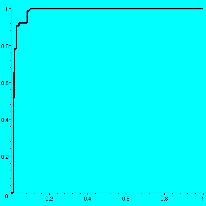
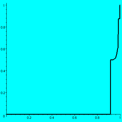
The associated graph is shown and it has approximate area .57585733. One surprising aspect of the graph to me was the enormous flatness of most of it: but of course the graph is not "flat" anywhere (any interval has infinitely many rationals, so the graph must increase). The amount of increase is mostly very very very small. Maple also displays the vertical jumps with vertical line segments. I don't know or understand very much about the possible values of int01f. It is between 0 and 1, but it can be very very large: if I select the first 30 "random" rationals close to 0, then I get the first graph shown below and the area is .97827779, and if I select the first 30 "random" rationals close to 1, then I get the second graph shown below and the area is .05210699.
Problem Is there a bijection B which has int01f=1/2? I don't know. In fact I don't know any specific value (or non-value!) of int01f. Certainly fairly easy reasoning (moving around the big blocks) shows that the values of int01f are dense in (0,1), but I really don't know the answer to the question just asked. I suspect it is "yes". | ||||||||||||||||||||||||||||||||
| 4/30/2003 |
Tomorrow I will give out student evaluation forms. Also tomorrow I
will request information on when I can usefully be available before
the final exam. The final is scheduled for
Tuesday, May 13, 12:00-3:00 PM in SEC 205
Historically probability has been the inspiration of many of the more intricate results about integration. I now take a small detour to present a complicated example of a function. First I tried to give some background on probability. Probability originated in the 1600's in an effort to predict gambling odds. Here's the basic idea, as it is now understood. One plays a game "many" times and observes the outcomes. A quotient called the "relative frequency" is computed: this is the (number of outcomes of a desired type) divided by (total number of times the game has been played). Of course relative frequency is a number between 0 and 1. Now the idea or hope or desire is that as the(total number of times the game has been played) gets large (approaches infinity?) this relative frequency should somehow "stabilize" or approach a limit. This limit is called the probability of the outcome of the desired type. Since the limit of a sequence of numbers in [0,1] is also a number in [0,1], the probability of a collection of outcomes is always in [0,1]. Of course this is all a model of reality, and building these models can be difficult. And certainly the relevance to "reality" of what's deducted using these models can also be debated. But that's the basic idea. Now I'll introduce some vocabulary and illustrate the vocabulary with a few examples.
Note 1 Here is one unpleasant consequence of this model. Since the probabilities of all the outcomes in the sample space should add up to 1, there is no positive number "left over" to assign as the probability of Tinfinity (since the sum of 1/2n as n goes from 1 to infinity is 1), so its probability must be 0! So here is a conceivable event which happens hardly ever, according to this model. Note 2 This "game" is called "choosing a number from the unit interval uniformly at random". Clearly (?) the correct model would assume that the probability of an "interval event" is the length of the interval. Being subintervals of [0,1] means that the lengths are correctly weighted so the probability of the whole sample space is 1, as it should be. But then the probability of, say, the event which is the interval (1/3-1/n,1/3+1/n) is 2/n for all positive integers n. Then since pr({1/3})<=pr((1/3-1/n,1/3+1/n)) should be true (smaller events should have smaller probabilities!) we see that pr({1/3})<=2/n for all n in N. Thus (Archimedean property!) pr({1/3})=0 in this model. What is more unsettling to realize is that the probability of any one number event is 0! So the chance of picking any one number, according to this model, is 0, but we've got to pick some number! Both note 1 and note 2 deal with the paradoxes of trying to model infinite "games" with a series of rules that lead to weirdness. These weirdnesses seem to be necessary. The most famous results of probability deal with repeated experiements and the tendency of random variables to have nice "asymptotic" properties. One such result is the Central Limit Theorem, which essentially states that the normal curve rules every repeated experiment. Here are two applets simulating the CLT, one with dice and one with a sort of pachinko-like "game". Such results are usually understood and investigated using the cumulative distribution function, cdf, of a random variable X. So cdf's are extremely important in probability.
If X is a random variable, the cumulative distribution
function, f of X is defined by this: Some effort is needed to be acquainted with this definition. Let's look at our three random variable examples, and graph their cdf's.
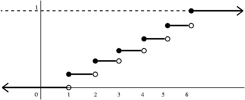
Tossing a fair die Here there are jumps of 1/6 at 1 and 2 and 3
and 4 and 5 and 6. A graph of the cdf follows. There is a solid dot
where the value of the function is, and an empty circle where it "isn't".
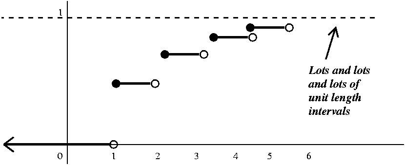
Flipping until a head occurs Here there are jumps of 1/2 and 1/4
and 1/8 and ... at 1 and 2 and 3 and ... This graph takes some
thinking about.
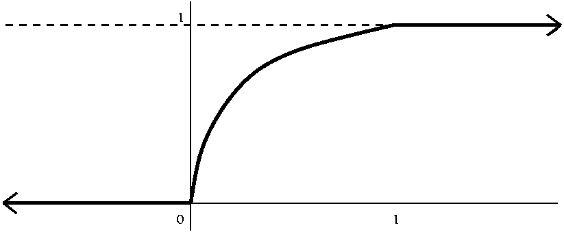
Squaring a uniformly distributed number from [0,1] What is the
probability that such a number is less than 1/2? This is the same as
asking for the length of the interval of x's in [0,1] for which
x2<=1/2. That interval is [0,1/sqrt(2)], so its length
is 1/sqrt(2). Therefore the graph is sqrt(x) for x in [0,1], and 0 for
x<0 and 1 for x>1.
Sometimes people say that properties 5 and 6 mean that the cdf is a cadlag function (!). This is an acronym for the French phrase "Continue a droite, limite a gauche": the function is continuous from the right, and has left-hand limits. We will discuss and further verify these properties tomorrow, and also try to count the number of jumps that any cdf can have. And we will look at a remarkable cdf. In the case of continuous random variables, another function is sometimes studied, the density function. This turns out to be the derivative of the cdf, and its utility for discrete random variables is not immediately clear. (What should the derivative of a mostly horizontal function be?) So I will just look at cdf's here, today and tomorrow. | ||||||||||||||||||||||||||||||||
| 4/28/2003 | Again we are going through the technicalities on integral and order,
integral and linearity, and additivity of the integral over intervals.
This takes effort and discipline, but Math 311 is the course
whose total object is constucting calculus (also called "analysis") with all
the interconnections showing. So let's move on and finish up these
technicalities.
Proposition (negating integrands) Suppose f is Riemann
integrable on [a,b]. Then the function h defined by h(x)=-f(x)
is also Riemann integrable on [a,b], and
intabh=-intabf. Initially I want to show that h is Riemann integrable. I will use the necessary and sufficient condition with epsilon. What do I mean? I must show that given epsilon>0, there is a partition P of [a,b] so that US(f,P)-LS(f,P)<epsilon. Since the upper sums and lower sums of f involve infs and sups, we can apply the previous remark. We get US(h,P)=-LS(f,P) and LS(h,P)=-US(f,P). Therefore US(h,P)-LS(h,P)=-LS(f,P)-(-US(f,P))<epsilon. We now know that h is Riemann integrable. We need to show that intabh=-intabf. Let's look at UI(h,[a,b]). This is inf of the upper sums of h. But each upper sum of h is minus a lower sum of f. Therefore the inf of h's upper sums is (again by the remark above!) equal to minus the sup of the lower sums of f. But this is -LI(f,[a,b]). Therefore we have shown that UI(h,[a,b])=-LI(f,[a,b]). Since f and h are Riemann integrable, the upper and lower integrals of each are equal to the "integral" of each. That is, we have verified intabh=-intabf as desired. Note This differs slightly from the presentation made in class. I believe it is more systematic, and perhaps better. I am not sure, though.
The last three propositions can be abbreviated by writing that:
Possible question of the day Suppose g is Riemann integrable on [0,5], and you are told that int05g=13, and that |g(x)|<=3 for all x in [0,2]. What over and underestimates can you make about int25g and why?
First was MEGO. The web site www.acronymfinder.com reports that this means "My Eyes Glaze Over (during a boring speech or briefing)". I asked for the source of the quotation "sup of the evening, beautiful sup" -- this was a misspelling of the word "soup" and the phrase comes from chapter 10 of Lewis Carroll's "Alice in Wonderland" where it is the first line of a song that the Mock Turtle sings. John Tenniel's historic illustration is shown. The Mock Turtle also discusses its education, and remarks that it studied `the different branches of Arithmetic-- Ambition, Distraction, Uglification, and Derision.' Lewis Carroll was actually an academic mathematician at Oxford University named Charles Lutwidge Dodgson. Biographical information is abundant. | ||||||||||||||||||||||||||||||||
| 4/24/2003 |
The Question of the Day Suppose f:R-->R is defined by f(x)=5 when x=3 and f(x)=-9 when x=6, while f(x)=0 for all other x's. Is f Riemann integrable on [2,7], and, if it is, what is the Riemann integral of f on that interval? Answers: Yes, and 0.
I began by observing that the special arguments last time actually
proved more than I stated. Comment The method of proof actually also provides the beginning of an algorithm to approximate definite integrals, so the work is not totally wasted, even though the conclusions of the theorem to be stated below apply to many more functions than this one. Corollary Suppose f is differentiable on [a,b], and there is K>0 so that |f'(x)|<=K for all x in [a,b]. Then f is Lipschitz and therefore Riemann integrable. We reconsidered an example discussed on 4/14/2003 (see the material on boxes and butterflies): the function sqrt(x) on the interval [0,1]. Since f'(x)=x-1/2 for x>0, the derivative is not bounded on (0,1]. And we actually saw that this f does not satisfy a Lipschitz condition on [0,1]. But everyone who has been through a calculus course knows that sqrt(x) for x between 0 and 1 does have an area, and this area is even easily computable with the Fundamental Theorem of Calculus. So how can we verify this function is Riemann integrable on [0,1]? The following result is a major success of the course.
Theorem (continuous functions are Riemann integrable) Suppose f
is continuous on [a,b]. Then f is Riemann integrable on [a,b].
We will use a simple partition again. So P will break up [a,b]
into n equal intervals, each of length (b-a)/n. The number of boxes is
n. In each subinterval, the inf and sup of f on
[xj-1,xj] is actually assumed: there are numbers
mj and Mj so that sup of f on
[xj-1,xj] is Mj=f(pj) and
inf of f on [xj-1,xj] is
mj=f(qj). This is a consequence of continuity.
The difference between the upper and lower sums will be bounded
by:
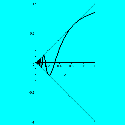
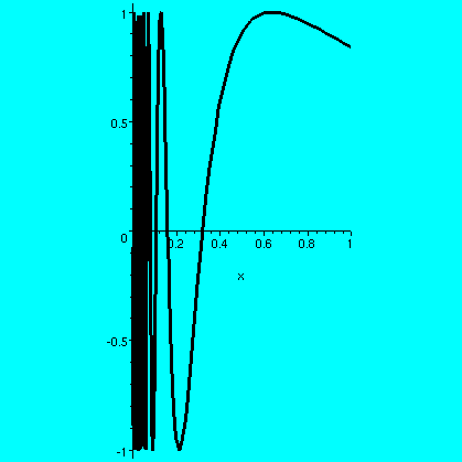
I will assume the standard properties of sine for these examples (we could instead get functions whose graphs would be polygons with similar properties, but would it be worth the trouble to define them?). Here is a picture of the function f(x)=sin(1/x) for x not 0, and f(0)=0. This function is continuous in [0,1]. If (xj) is any sequence in (0,1] with 0 as a limit, then the sequence (f(xj) is squeezed by the "x" and the limit will be 0. I had Maple draw in the "squeezing lines", +/-x, as well as sin(1/x) in this picture. This function has an infinite number of wiggles up and down in [0,1], but it is still Riemann integrable. Now consider the function sin(1/x) on (0,1]. A first observation is that there's no way to define this function at 0 so it will be continuous there. That's because it is possible to find sequences (xj) in (0,1] whose limits are 0 for which (f(xj) could be either a sequence without a limit, or sequences with different limits (it isn't hard to get explicit sequences converging to 0 or 1 or -1, for example). So there's no "natural" f(0). For simplicity, let's define f(0)=0. I claim that this f is indeed Riemann integrable on [0,1]. Here's is a verification of this claim.
This web page has links to notes of Professor Cohen which we are (approximately) following. Please look down the page and find "Riemann Integral, Section 1".
Plans ...
Theorem (order and integral) Suppose f and g are Riemann
integrable on [a,b], and that for all x in [a,b], f(x)<=g(x). Then
intabf<=intabg(x).
Corollary Suppose that there are real numbers m and M so that
for all x in [a,b], m<=f(x)<=M and f is Riemann integrable in
[a,b]. Then m(b-a)<=intabf<=M(b-a).
Linearity of the integral here will mean that
intabqf+g=q intabf+intabg
when f and g are Riemann integrable on [a,b] and q is a constant. I
will divide this into three parts, allowing me to concentrate on
smaller steps:
Proposition (i) Positive homogeneity)
Suppose q is a positive constant and f is
Riemann integrable on [a,b]. If g is a function defined by
g(x)=q·f(x), then g is Riemann integrable on [a,b] and
intabg=q·intabf. Now apply these observations to the collection of upper sums of g and the upper sums of f. Note that US(g,P)=qUS(f,P) because of the ideas above. So we have verified that UI(g,[a,b])=qUI(f,[a,b]). We can similarly verify that LI(g,[a,b])=qLI(f,[a,b]). Since f is Riemann integrable, UI(f,[a,b])=LI(f,[a,b]), implying that UI(g,[a,b])=LI(g,[a,b]), and therefore, g is also Riemann integrable. Whew! And we also know that the upper and lower integrals both multiply by q, so that intabg=q·intabg. | ||||||||||||||||||||||||||||||||
| 4/23/2003 |
We used the lemma proved last time to verify the following Theorem (upper sums dominate lower sums) If S and T are any partitions of [a,b], then US(f,S)>=LS(f,T). Proof: Here's the proof, which is very witty. Last time we proved that more points in the partition may make the upper sum decrease, but can't make it increase. A similar result (reversing directions, though!) is true for lower sums. Therefore, if P is the union of the partitions S and T, we have the following sequence of inequalities: LS(f,T)<=LS(f,P)<=US(f,P)<=US(f,S). The central inequality (between LS and US for P) is true because sups are bigger than infs, always.
Comment I can't imagine a totally convincing picture of the
situation addressed in this result -- it seems really complicated.
Temporarily, I defined:
A=the set of all lower sums of f. That is, x is in A if
x=LS(F,P) for some partition P of [a,b].
The theorem just stated presents us with a situation which should be
familiar from earlier work in the course (a month or more ago). The
sets A and B have the following properties: if a is in A, then a is a
lower bound of B, and if b is in B, then b is an upper bound of A. It
is natural to look at the sup of A and the inf of B. Here we will use
special phrases: If f is example 3 of the last lecture (0 on the irrationals, and 1 on the rationals, and the interval is [0,1]) then A={0} and B={1}, not very big sets, and not very complicated!
How can we tell if the Riemann integral exists, and how can we get
interesting examples? We will begin with this theorem: Now we need to verify the "epsilon condition" implies Riemann integrability. Remember what the sets A and B are. Since every element of B is an upper bound of A, and every element of B is a lower bound for A, we already know that sup A<=inf B. Why is this true? Well, if sup A>inf B, then take epsilon= sup A-inf B>0. We can find (sup chracterization) a in A so that sup A>=a>sup A-epsilon. a is then greater than inf B=sup A-epsilon. But we could then (inf characterization) find b in B with a>b>=inf B, which contradicts the known fact that a<=b for all choices of a in A and b in B. How can we prove Riemann integrability? This condition is exactly the same as proving sup A=inf B. Since we already know sup A<=inf B, let us see what happens when sup A<inf B. Then take epsilon=inf B-sup A>0. The assumption in the statement of the theorem says we can find a in A and b in B with b-a<"this" epsilon. So b-a<inf B-sup A. But certainly a<=sup A and inf B<=b, yielding (since -sup A<=-a) inf B-sup A<=b-a. This is a contradiction! Whew. (The logic in all this is a bit intricate, but is very similar to lots of proofs we did a month or two ago.)
Even better is the following result: With this result (whose proof I postponed until next time) we will actually be able to effectively recognize some Riemann integrable functions and maybe compute some integrals.
| ||||||||||||||||||||||||||||||||
| 4/21/2003 |
The problem of area What is area? This is a serious geometric question and difficult to answer. Usually we would like "area" to be something satisfying the following rules:
Just an initial statement of these properties is awesome. What is more distressing is the following statement, whose verification needs more time than this course has to run: there is no way to assign area to every subset of the plane in a way that obeys all of the rules above. This is irritating. In R3 the situation is even worse. It turns out that some "obvious" facts about decomposition of polyhedra into pieces with equal area are also not true! There is more information about this in Hartshorne's book. Here we do something much more pedestrian. We will try to assign "area" (actually, the definite integral) to regions in the plane bounded by the x-axis, x=a, x=b (here a<b) and y=f(x). Even for this seemingly more modest goal will turn out to be more difficult than one thinks, and the examples we will consider will be intricate and irritating.
We will start with a function f defined on [a,b]. We need to split up the interval. The word "partition" is used both as a verb and as a noun in this subject. As a verb, partition means to break up the interval into subintervals. As a noun, currently more important, "partition" P will mean a finite subset of [a,b] which contains at least both a and b. So a partition could be as small as just {a,b} (I'll assume here that a<b, so a and b are distinct). Or a partition could have 10100 points. The points in P will usually be written here as {a=x0<x1<x2<...<xn-1<xn=b}. In this case the partition has n+1 elements, and it has divided the interval into n subintervals (although frequently the subintervals have equal length, this is not required). The mesh of the partition P will be written ||P|| and it means the maximum of xj-xj-1 for j running from 1 to n. Since P is a finite set, the word "maximum" can be used, and will equal one of the elements of the set. Additionally, we will need to specify "tags" (word used in the text) or "sample points" (phrase I am more used to). So this is a selection of tj in each subinterval [xj-1,xj] as j runs from 1 to n. The tj will be used to create the height of each subrectangle. Then the Riemann sum of f on [a,b] with partition P and sample points T is sumj=1nf(tj)(xj-xj-1). The idea is that as ||P||-->0, this sum should tend to some sort of limit, and this will be the area or the definite integral. We'll call this RS(f,P,T): it is a complicated creature. I will return to this general sum later, but right now I will try something which may be a bit easier to handle: upper and lower sums.
The Upper Sum of f on [a,b] with partition P, US(f,P), is
sumj=1n(sup of f on [xj-1,xj])(xj-xj-1).
Example 2 f(x)=1 if x=1/2 and f(x)=0 otherwise. On the interval [0,1] use the partition {0,0,1/2-1/n,1/2+1/n,1}. This partition has four points and three subintervals. The lower sum is 0 because the infs on any of the three subintervals is 0. The upper sum has three parts. The left and right parts are 0 because the sup is 0 there, but the inside part, with width 2/n, has sup=1. Hence the upper sum is 2/n. The difference between the upper and lower sums here also-->0 as n gets large. Example 3 Consider the function f which is 0 on all of the irrationals and 1 on all the rationals. Then since there are rationals and irrationals in all intervals of positive length (the "density" of the rationals and irrationals) all of the upper sums on the interval [0,1] are 1 and all of the lower sums on the interval [0,1] are 0. There is always a discrepancy of 1 between the upper and lower sums. Definition The Upper Riemann integral is the inf of all of the upper sums of f. The Lower Riemann integral is the sup of all of the lower sums of f. We will say that f is Riemann integrable if the upper and lower Riemann integrals are equal. The common value will be called the Riemann integral of f. So the functions of examples 1 and 2 are Riemann integrable, with integrals of value 1/2 and 0 respectively. The function in example 3 is not Riemann integrable.
The following result plays an important part in any development of the
Riemann integral. On Wednesday I hope to give out some notes written by Professor Cohen which will outline this material. | ||||||||||||||||||||||||||||||||
| 4/16/2003 |
The instructor addressed the question, "Where do we go from
here?" and then answered even more inquiries in preparation for the
exam. I brought in the text (a standard calculus book) used for Math 151 and compared what's in Chapter 6 of the Math 311 textbook with that text. The approach and even many of the pictures, are the same. What happens?
In the balance of time remaining for the class I tried to answer more questions in preparation for the exam. Maybe the only interesting comment was my remembering a "workshop" problem from calculus. The problem was something like this: Aliens change and permute 10,000 values of the function F(x)=x2. That is, they might change (2,4) and (5,25) to (2,25) and (5,4), except that this is done to 10,000 points. What is the value of limx-->aF(x) and why? The answer is that limx-->aF(x) exists for all a's, and its value is alway a2. This is rather surprising, but once one is "close enough" to a (and not equal to a)there is no difference between the original function and the altered function. I worked on some other textbook and workshop problems, just as I had in the review session the night before. |
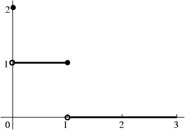 This version of FTC has to do with how the integral behaves as a
function of its upper parameter. Perhaps an example will make the
difficulties clearer. Let's look at a function defined in [0,3] by the
"piecewise" formula f(0)=2, f(x)=1 for 0<x<=1, f(x)=0 for
1<x<=3. We first observed that f was indeed Riemann integrable
on [0,3]. We could use partitions such as {0,B,H,C,3} where B is
slightly bigger than 0, H is slightly less than 1, and C is slightly
larger than 1. The difference between the resulting upper and lower
sums is "very small". And consideration of such sums allows one to
actually compute the Riemann integral. Of course f is also Riemann
integrable on subintervals of [0,3], so we could define F by
F(x)=int0xf for x in [0,3]. We can actually
"compute" F. First, F(0)=int00f must be 0,
because the width of the "subintervals" in any Riemann sum must be
0. Now if x is between 0 and 1 (or actually equal to 1) we can use the
partition {0,B,1} with B close to 0 to see that
int0xf is x (really, the width of 1-B is close
to x and the height, sup of f on [B,1], is 1). Now if we have x>1
and x<=3, we can use the partition {0,B,H,C,3} as before to see
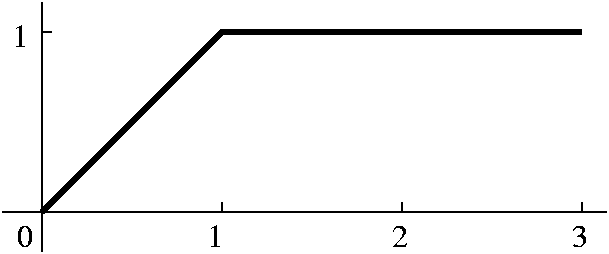
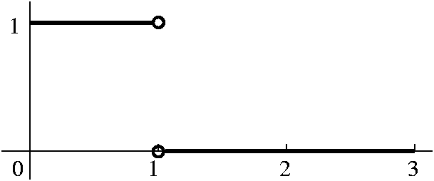
that for such x's, F(x) is 1. What about the derivative of F? Everyone
who has gone through a calc 1 class can tell that F is differentiable
for x in [0,1) and its derivative is 1, and it is also differentiable
in (1,3] with derivative 0. To the left below is a graph of F, and to the
right below is a graph of F'. I would like you to compare F' and
f. The Riemann integral, by the way, doesn't even "notice" the
discontinuity of f at 0. The Riemann integral locally averages the
behavior of f and reports that local average to F.

 Several (dubiously) interesting (?) linguistic comments were made
during today's class.
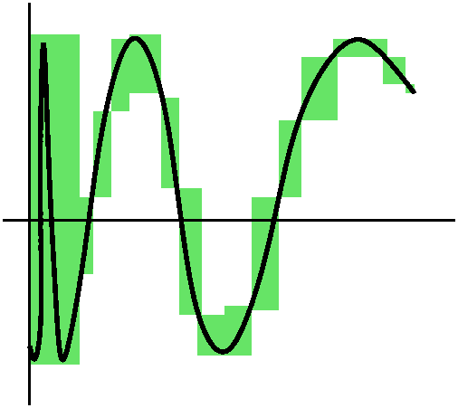 Given epsilon>0, we need a partition P of [0,1] so that
US(f,P)-LS(f,P) is less than epsilon. The maximum height
of any box in that difference is 2 since the range of sine is [-1,1].
So let's "waste" epsilon/2 on a first box: take 0 and x1 so
that x1<epsilon/4. Then the upper-lower on that
subinterval must be less than (epsilon/4)·(maximum
height)=epsilon/2. Now consider sin(1/x) on the interval
[x1,1]: there the function is continuous, hence Riemann
integrable, and there is a partition Q of [x1,1] so
that US(f,Q)-LS(f,Q)<epsilon/2. Now take P to
be the points in Q together with 0, and the discrepancy will be
at most the sum of the two, so therefore we have the desired partition
whose difference between upper and lower sums is less than epsilon. A
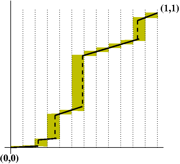
picture may help understanding. The large vertical box all the
way on the left of the picture contains infinitely much
wiggling of sin(1/x). The finite amount of wiggling not contained in
that box is "captured" inside a finite sequence of other boxes.
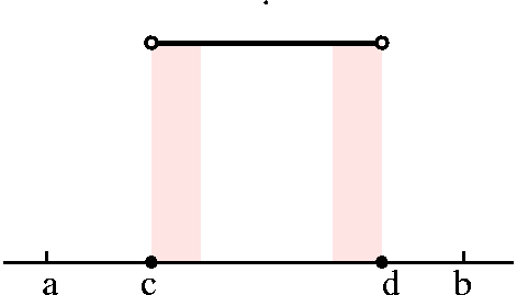 Example 1 A step function: Select numbers
a<c<d<b. Define the function f(x) by f(x)=1 if c<x<d,
and f(x)=0 otherwise. This is the simplest example of what the text
(and other sources) call a step function. With some effort, we
decided to look at the following partition:
P={a,c,c+(1/3n),d-(1/3n),d,b}.
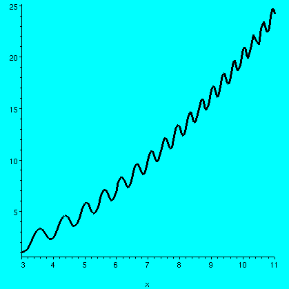 Example 2
f(x)=(1/5)x2+arctan(cos(x2).
 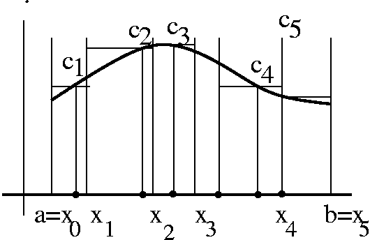 We will follow the lead of Cauchy and Riemann in this. Bressoud's book
(referenced in the general background to the course) discusses some of
Cauchy's ideas and shows that some of what Cauchy wrote was just
wrong! This stuff can be difficult. The basic idea is exactly
described by the picture to the right, which is almost surely rather
familiar to every student who has been through a basic calculus
course. We need to label and define and investigate every aspect of
this picture. I note that we are investigating what is called the
Riemann integral (Google has over 72,000 responses to "Riemann
integral"). Another candidate for integration is called the "Lebesgue
integral" (Google has over 29,700 responses to "Lebesgue
integral").
 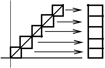 Example 1 f(x)=x, [0,1]. Here I looked at the partition
P which was {0,1/n,2/n,3/n,...,(n-1)/n,1}, an evenly spaced
partition dividing [0,1] into n equal subintervals. The difference
between the upper and lower sums can be exactly computed in
this case (most unusual, because almost always we will need to
estimate such things). Just "shove over" the boxes so they line up and
have height 1 and width 1/n, so that the difference between the upper
and lower sums is 1/n. As n gets large, this discrepancy -->0.