Celestial Mechanics
J. Massimino
History of Mathematics
Rutgers, Spring 2000
Throughout the history of mathematics, branches of scientific
study have regularly used mathematical methods to explain natural
phenomena. This is very true in the field of astronomy, and
particularly in the case of celestial mechanics.
Celestial mechanics is defined as
the branch of astronomy dealing with the mathematical theory of the
motions of celestial bodies. The curiosities of celestial mechanics
date back in to ancient times. The ancient Greeks, for instance,
gave divine status to the cosmos, and therefore felt the need for
further exploration. At this time, astrology established itself and
became a part of everyday life. The principle that stars could
influence man's life "...received some kind of justification from the
notion of cosmos, a cosmos which is so well arranged that no part is
independent of the other parts and of the whole. Was this not proved
by the tides, caused by Moon and Sun, by the menstruation of women, by
the farmers' moonlore... (Sarton, 165)." During the third century BC,
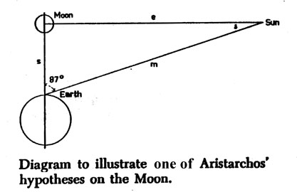
Aristarchos of Samos combined Euclidean geometry with the assumption that
the Sun is the center of the "universe" rather than the Earth1.
In his model
the planets circle the Sun, the Moon orbits the Earth, and
the stars are fixed, while their apparent "rotation" is an illusion caused
by the Earth's rotation. This heliocentric model was later reaffirmed
by Nicholas Copernicus (c. 1520).
In the late 17th century, a new age of thinking, now called the
Enlightenment, began. During this Age of Reason, intellectuals looked
for a single principle that would join together the concepts of
nature, God, and reason2.
Sir Isaac Newton (1642-1727) of Great
Britain made a major contribution to the scientific world during this
time with the publication of his greatest work, Philosophiae Naturalis
Principia Mathematica, later referred to simply as
Principia. In this
great work Newton discussed many influential
ideas, including his famous Laws of Motion, which dramatically
affected the understanding of celestial mechanics. These laws are:
- That every body continues in its state of resting or of
moving uniformly in a straight line, except insofar as it is driven by
impressed forces to alter its state.
- That the change of
motion is proportional to the motive force impressed, and takes place
following the straight line in which that force is impressed.
-
That to an action there is always a contrary and equal reaction;
or, that the mutual actions of two bodies upon each other are always
equal and directed to contrary parts.
These laws became essential in the study of mechanics of bodies in
space. These laws were combined with the law of gravity, which was
an essential factor for further discoveries in celestial mechanics.
The gravitational factor established in this law was an important
component of the works of a key 18th century mathematician,
Joseph-Louis Lagrange.
The Life of Joseph-Louis Lagrange4
Joseph-Louis Lagrange was born on January 25, 1736 in Turin to an
influential family. At the age of fourteen, Lagrange was sent to the
University of Turin to study law, after his father went bankrupt after
poor financial speculation. Although he was to
study law, his interests and abilities quickly showed to favor
mathematics, especially math analysis. Justly so, Lagrange was
appointed substitute professor at the Royal Artillery School in Turin
in 1755, and only two years later established the Royal T urin Academy
of Sciences with his colleagues, chemist Count Saluzzo di Monesiglio
(1734-1810) and anatomist Giovanni Cigna (1734-1790). However, in
1766, Lagrange grew unhappy with the limited research resources
available in Turin, and so, moved to Berl in where he was installed as
Director of Mathematics in the Berlin Academy. His years in Berlin
proved to be the most fruitful period of his life. "During this time,
he wrote on all branches of mathematics and intensively studied
mechanics. The majorit y of his memoirs during this period deal with
celestial mechanics (Lagrange, xix)." The writings from these memoirs
were submitted to the Académie des Sciences de Paris, whose major
scientific questions during the Enlightenment focused around:
-
describing mathematically the motion of the Moon,
- accounting for the
apparently secular inequality in the motions of Jupiter and Saturn,
-
determining the precise shape of the Earth.
Lagrange's writings on
these topics won competitions held by the Académie five times, which
helped to further establish him as a prominent mathematician of the
time.
With political changes occurring in Berlin in 1786, Lagrange
again became unhappy and dissatisfied and so accepted the position of
pensionaire vétéran of the Académie des Sciences, causing him to move
to Paris. In less than a year later, the first e dition of Lagrange's
most famous work, Mécanique Analytique, was published. This book
dealt with his findings about principles of statics and dynamics and
eventually laid the groundwork for further studies in mechanics.
Lagrange continued his studies in Paris, despite the fact that the
French Revolution (c. 1789) was all around him, even through to his
death in 1813. Just prior to his death, Lagrange summarized his life
with these words:
" Death is not to be dreaded and when it comes
without pain, it is a last function which is not unpleasant. I have
had my career; I have gained some celebrity in mathematics. I never
hated anyone, I have done nothing bad, and it would be well to end
(Kramer 220)."
The second edition of Mécanique Analytique, which
expands upon the works of the first, was published posthumously in
1815.
The Works of Joseph-Louis Lagrange5
In the second edition of Mécanique Analytique, Lagrange's work
focused more on celestial mechanics than the previous edition had. In
this edition, Lagrange produced equations6
aiding the understanding of
celestial mechanics, including those dealing with:
- Orbital Shapes
- Planetary Periods
- Changes in Orbits when a Planet is subjected
to an Arbitrary Impulse
- Perturbations
- Orbital Shapes7
In the world system, according to Lagrange, the force of attraction
is inversely proportional to the square of the distance.
R= g/r2 =>  R dr=-g/r
Using the equation between F
and r, the substitution
becomes
R dr = 2H + (2g/r) - (D2/r2).
Then the polar equation of the
conic section with parameter b and eccentricity e is
r = b/(1+ ecosF
given that b = D2/g ,
and e = [1+ (2HD2/g2)]1/2.
Lagrange calls the
average distance a, so that a = b/(1-e2).
Using simplification and
substitution with D and H,
the new relationship is
1/a = (1-e2)/b = -2H/2g,
where the constant H must be negative in order to produce an
elliptical orbit. If H were zero, the orbit would be parabolic, and
if H were positive, the orbit would be hyperbolic.
Planetary Periods
In order to compute the period of a planet, Lagrange began with the equation
dt = dr/ [(2H-(2R dr)
- D2/r2)]1/2
Using the substitution
dt = (r dr) / ([ga]1/2 [e2-(1-r/a)2]1/2), and
r = a(1-e cosq
), we have
dt = [a3/g]1/2
(1-ecosq
dq
After integration,
t-c =
[a3/g]1/2
(q-e sin q),
thus giving q
as a function of t, and therefore, r as a function of t.
Lagrange then made a substitution into dt
using F.
This became:
dF =
dq
(1-e2)/ (1- ecosq) =>
F=
sin-1
(sinq[(1-e2)]1/2/(1-ecosq)) + constant.
Through a comparison of the expressions for r,
F
as functions of q,
b/(1+ecosF)
= a (1-ecosq).
Because b=a(1-e2),
Lagrange concluded cosF =
(cosq - e)/
(1 - e cosq),
sinF=(sinq)
[(1-e2)]1/2/(1-ecosq),
and thus, tan (F/2) = [((1+e)/(1-e))]1/2tan (q/2).
Lagrange concludes,
"It is clear from these formulas that when the angle
qis increased by
360 degrees, the radius r remains the same but the angle
F is also
increased by 360 degrees. Therefore, the planet returns to the same
point after having completed an entire revolution. But since the
angle q
has increased by 360 degrees,
the time t will increase by
360(a3/g)1/2.
This is the time required for the planet to return to the
same point in its orbit. Hence, this amount of time is called the
planet's period ... ." (Lagrange, 325)
Expressing Orbits in Terms of x, y, z
Recalling that r(1+ecosq)=b
and r=a(1-ecosq),
Lagrange substituted
in X=a(cosq - e),
so that X= (b-r)/e = (a(1-e2)-r)/e. Therefore,
X=a(cosq - e) and
2)]1/2sinq.
Using these expressions for X and
Y, Lagrange concluded that it was possible to substitute these
expressions in the general expressions for x,y,z, for which he
claimed,
" Thus, it will only be a question of substituting the
expression for ? as a function of t, obtained from the equation given
in Article 169 in order to obtain the three coordinates as functions
of time (Lagrange, 326)",
yet he never demonstrates this substitution.
Changes in Orbital Elements When a Planet is Subjected to an Arbitrary
Impulse
Up to this point, Lagrange had shown how to express the elements of
elliptical orbits using the functions of x,y,z and of their
differentials dx/dt, dy/dt, and dz/dt. However, it was observed that
planets were subject to impulses which affected the veloci ties.
This, Lagrange concluded, could be accounted for by the following
adjustments:
dx/dt --> dx/dt + x.
dy/dt --> dy/dt + y.
dz/dt --> dz/dt + z.
This gave the new elements of the planetary orbit
after the impulse.
Then using the radius vector
r, y, and
r
Lagrange
rewrote the elements of the orbits as:
1/a = 2/r -( r2(cos2y
dr2 + dy2)
+ dr2)/ g dt2
b = r4(cos2ydr2 + dy2)/gdt2
tan h =
(sinrdy -
sinycosycosrdr)/
(cosrdy -
sinycosysinrdr)
tan i = [(dy2 +sin2&#cos2ydr2)/(cos2ydr)
where
"dr/dt, rdr/dt,
and rdy/dt are
velocities in the direction of the radius r, in a direction
perpendicular to this radius and parallel to the plane of projection,
and in a direction perpendicular to this same plane (Lagrange, 361)."
Elements of Motion Produced by Perturbing Forces
Although the previous equations worked for arbitrary, momentary
impulses, Lagrange realized that it was necessary to compensate for
impulses that are infinitesimal and continuous, or perturbation
forces.
His work on perturbation forces begins:
"Let X,Y,Z, be the
perturbing forces resolved in the directions of the rectangular
coordinates x,y,z and having a tendency to increase the coordinates.
These forces will create during the instant dt the small velocities
Xdt, Ydt, Zdt which should be adde d to the velocities dx/dt, dy/dt,
dz/dt in the expression for each of the elements... because the added
velocities are infinitesimal they will only produce in the elements
infinitesimal variations which can be determined by the differential
calculus (Lagr ange, 367)."
Allowing the following definitions,
dx/dt = x', dy/dt = y', dz/dt = z',
Lagrange concluded that each of the elements of the orbit could be
expressed using x, y, z, x', y', z'.
If a is one of these elements,
then it "... will have its variation da by augmenting x', y', z' of
the infinitesimal quantities Xdt, Ydt, Zdt.
Thus one will have
da = (da/dx' X + da/dy' Y + da/dz' Z) dt
and similar equations will be obtained for the other elements ...
(Lagrange, 367)."
This work on the perturbation theory became a significant part of
the future of celestial mechanics.
Conclusion
With the development of Lagrange's equations for perturbations,
significant developments have occurred. It was through the use of
perturbation theory that Neptune was discovered. When astronomers of
the mid-nineteenth century observed a perturbed orbit of Uranus,
"astronomers Adams and Leverrier independently came to the conclusion
that the perturbation must be due to a planet as yet unknown to
astronomers (Kramer, 221)." This planet was soon discovered and named
Neptune. The discovery of Pluto in th e twentieth century was
similar.
Celestial mechanics has developed greatly throughout many centuries
of observation. From a time where the cosmos were used to explain
daily activity to the time of the Enlightenment when knowledge of how
the universe worked was desired, it is an ever re levant field. The
work of Joseph-Louis Lagrange, during the Enlightenment, proved to be
a prominent and fruitful assets to our current understanding of the
world.
Bibliography
- Densmore, Dana. Newton's Principia. Santa Fe, N.M. : Green
Lion Press, 1995.
- Kramer, Edna E. The Nature and Growth of
Modern Mathematics. Princeton, NJ : Princeton University Press,
1981.
- Lagrange, Joseph-Louis. Analytical Mechanics. Boston, MA
: Kluwer Academic Publishers, 1997.
- Moulton, Forest Ray. An
Introduction to Celestial Mechanics. New York, NY. : Dover
Publications, 1970.
- Sarton, George. Hellenistic Science and Culture
In The Last Three Centuries BC
Mineola, NY : Dover Publications, 1993.
- Smith, D.E. History of Mathematics. New York, NY: Dover Publications,
1951.
- Vinti, John P. Orbital and Celestial Mechanics. Reston, VA: American Institute
of Aeronautics and Astronautics, 1998.
Table of Variables
- R: the force of attraction
- g: gravitational force
- r: radius vector
- F/dt: the angle that r makes with a segment of the major axis from
the focus to the nearest vertex
- a: the average distance between the maximum and minimum of r
- t: time
- q/dt: polar quantity of an angle
- y/dt: the inclination of r on the xy-plane
- r/dt: the angle made by the projection of r on the plane
- H: T + V , where T is the kinetic energy and V is the potential
energy.
- i: an angle made by the plane of the curve Ax+By+Cz=0 and the
xy-plane
- h: the angle made by the same line of intersection of i with the
x-axis.
- D: C/cos i
Notes
- As shown below
- From Translator's Introduction to Mécanique Analytique.
- As translated from Principia.
- The biographical information used here is taken from the
Translator's Remarks of Mécanique Analytique and from the work
of Edna Kramer.
- As translated from Mécanique Analytique.
- Lagrange does not provide diagrams with his work, because he felt
that algebra was more appropriate than Euclidean geometry in these
computations.
- Please refer to the table of variables given above when following
the computations.
- Lagrange, pages 322-324.
- This is the equation t-c = [a3/g]1/2
(q
-e sin q)