Matrix multiplication appears naturally in many problems modeled by mathematics. For instance, a matrix can represent the transition of one population to a new one after a period of time; then repeated transitions correspond to successive multiplications of the matrix. Or a complex process of decomposition can be broken up into individual pieces, each of which represents a transition from one state to another; if the transitions are linear, then they can be represented by matrices, and the product of the matrices corresponds to the complex transition made up of those individual pieces. We consider several examples.
Population Change and the "Leslie Matrix"
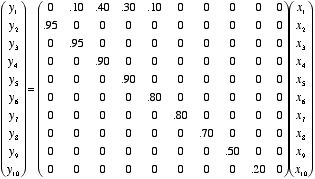
If we consider a definite population, it may be important to measure, or predict, its change over a period of years. If that population is isolated, then changes are due to births and deaths alone, and the age distribution of the population clearly has a key influence. Suppose, e.g. that we have a population that lives up to age at most 100 years, has well understood mortality rates at each yearly interval, and well understood reproduction rates during certain of those years. If we let [x1, . . ., x100] denote the vector measuring the population at each of the ages 1 through100 at a given time (we round age up to the nearest year), and consider what happens after 1 year, notice that the new distribution [y1 ,. . ., y100], for each of the numbers y2 through y100, will be determined by the survival rates for the corresponding ages one younger, that is, one index lower (x1 through x99 respectively), whereas y1 will be determined by the reproduction rates corresponding to the reproducing years. We consider a simplified example (using units of 10 years rather than 1 year, with x1 representing the number in the population under age 10, x2 the number between ages 10 and 20, etc.). Assume mortality rates (over 10 years) of .05, .05, .1, .1, .2,.2, .3, .5, and .8 (representing the transitions (under 10s)-to-(under 20s), (under 20s)-to-(under 30s), etc.), and reproduction rates of .1, .4, .3, and .1 in the under-20s, under-30s, under-40s, and under-50s age ranges, respectively. Then the following matrix equation expresses the 10-year transition from a given population distribution to the subsequent population distribution:
If we write this expression as y
= Ax, and if x represents the population distribution
at some initial measurement time, then Ax
represents the population 10 years later,
AAx=A2
x
gives the population after an additional 10 years, and, in
general, Ak
x
represents the population after 10k years.
For the given matrix as shown above, it can be determined that, after
32 iterations (which corresponds to a period of 320 years),
we have (after rounding)
A32=
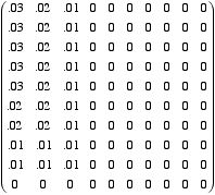
while after 64 iterations no entry is larger than 1/100, and after 1024 iterations no entry is larger than 10-35. On the other hand, if the reproduction rates are higher, for instance rates of .2, .5, .4, and .2 in the under-20s, under-30s, under-40s, and under-50s age ranges, respectively, then the matrices A and A32 (again, rounded) are as follows:
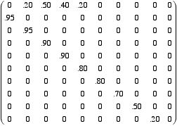 and
and 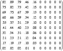 ,
,
while A1024 has entries in its first five columns all of which are between 1011 and 1014 , while the entries in the last five columns are all (rounded) zeros.
Unlike these two situations, there may be cases in which the limiting behavior of the powers of the matrices in question has interesting properties, other than entries which approach zero or infinity. Consider a simple 2 x 2 matrix, say
![]()
If we look for a population which is left fixed by
the action of this matrix, we find that there is
indeed a set of choices which works.
Flow Problems
Given a set of one
way paths with intersections and specified flow patterns through the
inte rsections (that is, fractions of the traffic which flows in each
of the possible directions our of the intersections),
it is possible to
break the analysis of overall flow out of the set of paths, based on
the amount flowing in, via a set of matrix computations. If, for
instance, there are three incoming flows, a set of one way paths
along a horzontal/vertical grid, and and ultimately two outgoing
flows, it is possible to determine the outgoing components
(a two vector) in terms of the incoming components (a 3-vector).
We consider an example with a set of 3 nodes at the first and
second steps, two nodes at the third
step, and analyze the resulting matrices (a total of three
describing the outputs past each node).
Selection Problems
Suppose a set of people (call them students) is to choose among a set of objects (call them courses); each student may select 4 or 5 courses from the list. A matrix A can be set up in which each chooser is represented by a row, each object is represented by a column, and the entries are either 0 or 1, depending on whether the chooser does not, or does, want the object. (Such matrices are called Adjacency matrices). An interesting set of information is encoded in ATA : notice that the (i, j) entry of ATA is the sum
a1i a1j + a2i a2j + · · · + anni anj
and the terms of this sum are zero, except when a student wants to take BOTH course i and course j, in which case the term is a 1. Thus the (i, j) entry of AT A is the total number of students who want to take both course i and course j; the (i, i) entries are the total number of students who want to take course i. Thus the main diagonal encodes information about the overall popularity of the courses, and the other terms allow a view of the most popular pair combinations, which can be used in terms of influencing the scheduling of such courses at different times.
