Lecture 2

In addition to addition and scalar multiplication, there is a third "multiplication" operation, a product that makes sense for matrices of certain related shapes. We begin with the case in which one of the matrices is, in fact, a vector.

Def. Let A = [a₁a₂ . . . a_n ] be an m x n matrix (here each a_j is a column vector of length n), and let v be a column vector of length n. The matrix-vector product Av is the column vector Av = v₁ a₁ + · · · + v_n a_n.

Examples

Note how we actually compute: the i'th entry of Av is a_{i 1} v₁ + · · · + a_{i n} v_n, which is computed from the i'th row of A and the entries in v.

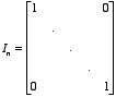
Note that multiplication of any n-vector v by the n x n matrix with entries equal to one on the main diagonal, and zero elsewhere, yields the original vector v again.

Def. The n x n identity matrix I_n, given by

The multiplication of a vector by a square matrix can be thought of as a transformation of the given vector into another vector. An important family of 2 x 2 matrices corresponds to the transformations consisting of rotations (counterclockwise) around the origin. If we think of the unit horizontal and vertical vectors , then it is easy to see that after rotation through the angle q, this pair of vectors must become the new pair . Thus we define the rotation matrices:

Def. The 2 x 2 matrix A_q, given by

,

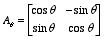As is fairly simple to verify, if u is any vector in R², then A _q u is the vector obtained after rotation of u counterclockwise through the angle q.

Matrix-Vector Product Properties

Let A and B be m x n matrices, and let u, v be vectors in Rⁿ. Then
(a) If e_j is the j'th standard vector (e_ji = 1 if j = i, and = 0 otherwise), then Ae_j = a_j is the j'th column vector of A.
(b) A(u + v) = A u + A v.
(c) A(cu) = c(Au) = (cA)u for all scalars c.
(d) (A + B)u = Au + Bu.
(e) If Bw= Aw for ALL w in Rⁿ , then B = A.
(f) A 0 = 0.
(g) Ov = 0.
(h) I_nv = v.

Note that all of these assertions are straightforward, except perhaps for (e). But ((e) follows from (a) because we can deduce that A and B have the same columns.

Systems of Linear Equations

We treat x₁, . . . , x_n as (real) variables, a₁, . . ., a_n as scalars (real constants), and can then consider the linear equation a₁ x₁ +. . . + a_n x_n = b, for a (real, constant) scalar right hand side. If we consider m such equations simultaneously, we have one of the fundamental problems of linear algebra: finding solutions to such systems.

Def. A system of linear equations is a set of equations of the form

Examples; including the general example of 2 equations in 2 unknowns.

How do we solve such systems, systematically? We replace the system by an equivalent one which is easier to solve. Such replacements correspond to the addition of two rows and the multiplication of a row by a nonzero scalar (and combinations of these operations), with the new row replacing one of the corresponding old ones, as well as the interchange of rows for bookkeeping purposes. The resulting systems are equivalent because the corresponding division and subtraction and interchanging would reverse the process.

Example

Now, we introduce a notational shorthand: Why carry around the variables x₁, . . ., x_n when we do not need to? Let A denote the matrix with entries a_ij as in the system above, let b denote the column vector with entries b₁, . . ., b_m, and let x denote the column vector with (variable) entries x₁, . . ., x_n. The system of linear equations can then be written as Ax = b. If we think of the operations that change this into an equivalent but simpler system, we note that the variable x appears in the same fashion all the time, so that it is really the matrix A and the vector b which we are changing. We form the augmented matrix of the linear system, [A b] (which we will sometimes write as [A | b] to emphasize that the last column has a different role than the others). The operations used to solve the linear systems can now be treated as operations on the augmented matrix, and we do not have to carry the variables along in the notation.

Def. The following operations on matrices are called elementary row operations:
1. Interchange two rows;
2. Multiply a row (that is, all of its entries) by a nonzero scalar;
3. Add two rows, replacing one of them with the sum.

In order to replace a given system of equations with one that we can easily solve, we note that we try to eliminate variables from the equations until we reach a point where the last variable is determined (or else free), and then back-substitute to find its predecessors.

Def. A matrix is in row echelon form if
(a) All zero rows (rows consisting of all zeros), if any, are below all other rows;
(b) For each row, the leading entry (the leftmost nonzero entry) is to the right of all higher rows' leading entries; and
(c) All entries in the column below any leading entry are zero.

Examples

Note that the corresponding linear system can be easily solved if the augmented matrix is in row-echelon form. It is arithmetically simplest if, in fact, each leading entry is a 1, which can be arranged by scalar multiplication. Moreover, if instead of back-substituting in solving a linear system, we first eliminate all earlier appearances of a given variable that will be determined, we have the simplest equivalent system to the original one. These operations correspond to the following form of the augmented matrix: