Exercise 15b of section 3.1 involves a function for which the repeated differentiation needed to express the error term requires care. A transcript of a Maple session for calculating these derivatives and applying the result to obtaining the error bound has been prepared. The third derivative of the expression appears in the error formula of the second degree interpolating polynomial. In the formula, the value of this derivative at an unspecified point in the interval appears, so that the largest absolute value of the function is used to compute the bound to be sure that any error is smaller. In order to get the estimate quickly, one usually overestimates the error since it is more satisfying to do the work of computing a better result than in needed than to put in more effort to justify not computing an extra term. In some cases, an additional derivative can be used to identify where the maximum of this quantity is attained, so a tighter estimate is possible. This is done for this example.
There is a second part of the error estimate that is a polynomial with roots at the points where the function is known exactly. For a given point at which the function is to be evaluated, one can put that value into this polynomial. However, if one is looking for uniform results over an interval, the maximum absolute value of this factor must be computed independently of the estimate described above. The product of these two bounds gives the uniform error approximation on the interval. This is computed. Then graphs showing the comparison of the function and the approximating polynomial are shown. Finally, since the function can be computed, we can examine the true error and show that it can be more than two-thirds of the bound that we found. This is close enough that there would be little benefit in seeking a tighter bound. (If the bound were more than ten times larger than needed, it might be worth looking for a better bound.)
If you want to repeat these calculations, and explore modifications, you can download (by holding down the shift key when you click the link) the Maple worksheet.
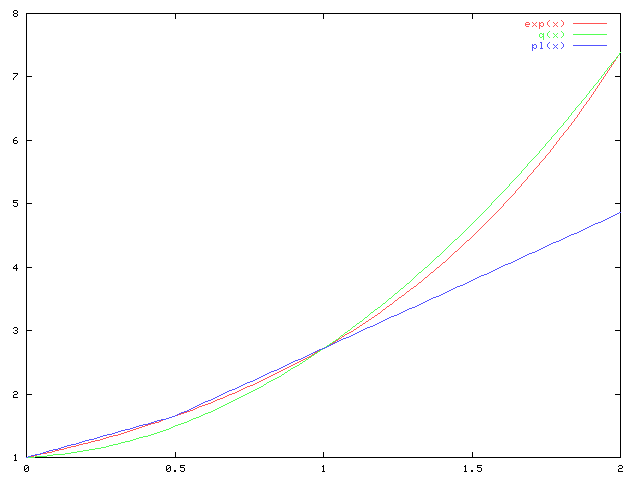
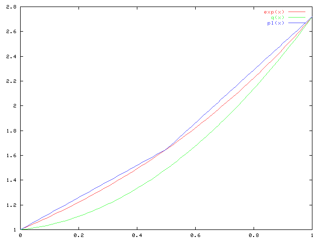
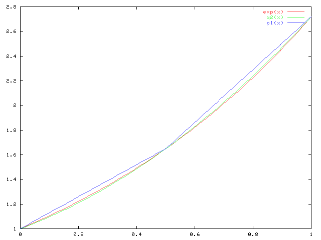
There are also some graphs of the exponential and its interpolating polynomials that allow a visual comparison of the error in these approximations. The first graph shows the exponential, the linear approximations, and the quadratic approximation for x between 0 and 2. This shows how the exponential and its quadratic approximation are very different even though they share threee common points. The second graph shows the same functions only between 0 and 1. The poor approximation of the quadratic polynomial at most points of this interval is seen. The linear interpolation between 0 and 1 is not shown, but can be easily imagined, and the quadratic polynomial shows no significant improvement over this weaker approximation. The use of the value of the exponential function at 2 leads to a poor fit between 0 and 1, so it would be more reasonable to use the value at 1/2 that was already used in the linear approximations. This is shown in the third graph. Not only is this quadratic an improvement over the linear approximations, but it has the advantage of giving a single smooth curve that approximates the exponential function over the whole interval between 0 and 1.